15

Large-Scale Algorithms

Large-scale algorithms are specifically designed to tackle sizable and intricate problems. They distinguish themselves by their demand for multiple execution engines due to the sheer volume of data and processing requirements. Examples of such algorithms include Large Language Models (LLMs) like ChatGPT, which require distributed model training to manage the extensive computational demands inherent to deep learning. The resource-intensive nature of such complex algorithms highlights the requirement for robust, parallel processing techniques critical for training the model.

In this chapter, we will start by introducing the concept of large-scale algorithms and then proceed to discuss the efficient infrastructure required to support them. Additionally, we will explore various strategies for managing multi-resource processing. Within this chapter, we will examine the limitations of parallel processing, as outlined by Amdahl’s law, and investigate the use of Graphics Processing Units (GPUs). Upon completing this chapter, you will have gained a solid foundation in the fundamental strategies essential for designing large-scale algorithms.

The topics covered in this chapter include:

• Introduction to large-scale algorithms
• Efficient infrastructure for large-scale algorithms
• Strategizing multi-resource processing
• Using the power of clusters/cloud to run large-scale algorithms

Let’s start with the introduction.

Introduction to large-scale algorithms

Throughout history, humans have tackled complex problems, from predicting locust swarm locations to discovering the largest prime numbers. Our curiosity and determination have led to continuous innovation in problem-solving methods. The invention of computers was a pivotal moment in this journey, giving us the ability to handle intricate algorithms and calculations. Nowadays, computers enable us to process massive datasets, execute complex computations, and simulate various scenarios with remarkable speed and accuracy.

However, as we encounter increasingly complex challenges, the resources of a single computer often prove insufficient. This is where large-scale algorithms come into play, harnessing the combined power of multiple computers working together. Large-scale algorithm design constitutes a dynamic and extensive field within computer science, focusing on creating and analyzing algorithms that efficiently utilize the computational resources of numerous machines. These large-scale algorithms allow two types of computing – distributed and parallel. In distributed computing, we divide a single task between multiple computers. They each work on a segment of the task and combine their results at the end. Think of it like assembling a car: different workers handle different parts, but together, they build the entire vehicle. Parallel computing, conversely, involves multiple processors performing multiple tasks simultaneously, similar to an assembly line where every worker does a different job at the same time.

LLMs, such as OpenAI’s GPT-4, hold a crucial position in this vast domain, as they represent a form of large-scale algorithms. LLMs are designed to comprehend and generate human-like text by processing extensive amounts of data and identifying patterns within languages. However, training these models is a heavy-duty task. It involves working with billions, sometimes trillions, of data units, known as tokens. This training includes steps that need to be done one by one, like getting the data ready. There are also steps that can be done at the same time, like figuring out the changes needed across different layers of the model.

It’s not an understatement to say that this is a massive job. Because of this scale, it’s a common practice to train LLMs using multiple computers at once. We call these “distributed systems.” These systems use several GPUs – these are the parts of computers that do the heavy lifting for creating images or processing data. It’s more accurate to say that LLMs are almost always trained on many machines working together to teach a single model.

In this context, let us first characterize a well-designed large-scale algorithm, one that can fully harness the potential of modern computing infrastructure, such as cloud computing, clusters, and GPUs/TPUs.

Characterizing performant infrastructure for large-scale algorithms

To efficiently run large-scale algorithms, we want performant systems as they are designed to handle increased workloads by adding more computing resources to distribute the processing. Horizontal scaling is a key technique for achieving scalability in distributed systems, enabling the system to expand its capacity by allocating tasks to multiple resources. These resources are typically hardware (like Central Processing Units (CPUs) or GPUs) or software elements (like memory, disk space, or network bandwidth) that the system can utilize to perform tasks. For a scalable system to efficiently address computational requirements, it should exhibit elasticity and load balancing, as discussed in the following section.

Elasticity

Elasticity refers to the capacity of infrastructure to dynamically scale resources according to changing requirements. One common method of implementing this feature is autoscaling, a prevalent strategy in cloud computing platforms such as Amazon Web Services (AWS). In the context of cloud computing, a server group is a collection of virtual servers or instances that are orchestrated to work together to handle specific workloads. These server groups can be organized into clusters to provide high availability, fault tolerance, and load balancing. Each server within a group can be configured with specific resources, such as CPU, memory, and storage, to perform optimally for the intended tasks. Autoscaling allows the server group to adapt to fluctuating demands by modifying the number of nodes (virtual servers) in operation. In an elastic system, resources can be added (scaling out) to accommodate increased demand, and similarly, resources can be released (scaling in) when the demand decreases. This dynamic adjustment allows for efficient use of resources, helping to balance performance needs with cost-effectiveness.

AWS provides an autoscaling service, which integrates with other AWS services like EC2 (Elastic Compute Cloud) and ELB (Elastic Load Balancing), to automatically adjust the number of server instances in the group. This ensures optimal resource allocation and consistent performance, even during periods of heavy traffic or system failures.

Characterizing a well-designed, large-scale algorithm

A well-designed, large-scale algorithm is capable of processing vast amounts of information and is designed to be adaptable, resilient, and efficient. It is resilient and adaptable to accommodate the fluctuating dynamics of a large-scale environment.

A well-designed, large-scale algorithm has the following two characteristics:

• Parallelism: Parallelism is a feature that lets an algorithm do several things at once. For big computing jobs, an algorithm should be able to divide tasks between many computers. This speeds up calculations because they are happening all at the same time. In the context of large-scale computing, an algorithm should be capable of splitting tasks across multiple machines, thereby expediting computations through simultaneous processing.
• Fault tolerance: Given the increased risk of system failures in large-scale environments due to the sheer number of components, it’s essential that algorithms are built to withstand these faults. They should be able to recover from failures without substantial loss of data or inaccuracies in output.

The performance of a large-scale algorithm is intricately linked to the quality of the underlying infrastructure. This foundation should provide adequate computational resources, extensive storage capacity, high-speed network connectivity, and reliable performance to ensure the algorithm’s optimal operation. Let us characterize a suitable infrastructure for a large-scale algorithm.

Load balancing

Load balancing is an essential practice in large-scale distributed computing algorithms. By evenly managing and distributing the workload, it prevents resource overload and maintains high system performance. It plays a significant role in ensuring efficient operations, optimal resource usage, and high throughput in the realm of distributed deep learning.

Figure 15.1 illustrates this concept visually. It shows a user interacting with a load balancer, which in turn manages the load on multiple nodes. In this case, there are four nodes, Node 1, Node 2, Node 3, and Node 4. The load balancer continually monitors the state of all nodes, distributing incoming user requests between them. The decision to assign a task to a specific node depends on the node’s current load and the load balancer’s algorithm. By preventing any single node from being overwhelmed while others remain underutilized, the load balancer ensures optimal system performance:

Figure 15.1: Load balancing

In the broader context of cloud computing, AWS offers a feature called Elastic Load Balancing (ELB). ELB automatically distributes incoming application traffic across multiple targets within the AWS ecosystem, such as Amazon EC2 instances, IP addresses, or Lambda functions. By doing this, ELB prevents resource overload and maintains high application availability and performance.

ELB: Combining elasticity and load balancing

ELB represents an advanced technique that combines the elements of elasticity and load balancing into a single solution. It utilizes clusters of server groups to augment the responsiveness, efficiency, and scalability of computing infrastructure. The objective is to maintain a uniform distribution of workloads across all available resources, while simultaneously enabling the infrastructure to dynamically adjust its size in response to demand fluctuations.

Figure 15.2 shows a load balancer managing four server groups. Note that a server group is a collection of nodes tasked with specific computational functions. A server group here refers to an assembly of nodes, each given a unique computational role to fulfill.

One of the key features of a server group is its elasticity – its ability to flexibly add or remove nodes depending on the situation:

Figure 15.2: Intelligent load balancing server autoscaling

Load balancers operate by continuously monitoring workload metrics in real time. When computational tasks become increasingly complex, the requirement for processing power correspondingly increases. To address this spike in demand, the system triggers a “scale-up” operation, integrating additional nodes into the existing server groups. In this context, “scaling up” is the process of increasing the computational capacity to accommodate the expanded workload. Conversely, when the demand decreases, the infrastructure can initiate a “scale-down” operation, in which some nodes are deallocated. This dynamic reallocation of nodes across server groups ensures an optimal resource utilization ratio. By adapting resource allocation to match the prevailing workload, the system prevents resource over-provisioning or under-provisioning. This dynamic resource management strategy results in an enhancement of operational efficiency and cost-effectiveness, while maintaining high-caliber performance.

Strategizing multi-resource processing

In the early days of strategizing multi-resource processing, large-scale algorithms were executed on powerful machines called supercomputers. These monolithic machines had a shared memory space, enabling quick communication between different processors and allowing them to access common variables through the same memory. As the demand for running large-scale algorithms grew, supercomputers transformed into Distributed Shared Memory (DSM) systems, where each processing node owned a segment of the physical memory. Subsequently, clusters emerged, constituting loosely connected systems that depend on message passing between processing nodes.

Effectively running large-scale algorithms requires multiple execution engines operating in parallel to tackle intricate challenges. Three primary strategies can be utilized to achieve this:

• Look within: Exploit the existing resources on a computer by using the hundreds of cores available on a GPU to execute large-scale algorithms. For instance, a data scientist aiming to train an intricate deep learning model could harness the GPU’s power to augment computing capabilities.
• Look outside: Implement distributed computing to access supplementary computing resources that can collaboratively address large-scale issues. Examples include cluster computing and cloud computing, which enable running complex, resource-demanding algorithms by leveraging distributed resources.
• Hybrid strategy: Merge distributed computing with GPU acceleration on each node to expedite algorithm execution. A scientific research organization processing vast amounts of data and conducting sophisticated simulations might adopt this approach. As illustrated in Figure 15.3, the computational workload is distributed across multiple nodes (Node 1, Node 2, and Node 3), each equipped with its own GPU. This figure effectively demonstrates the hybrid strategy, showcasing how simulations and computations are accelerated by capitalizing on the advantages of both distributed computing and GPU acceleration within each node:

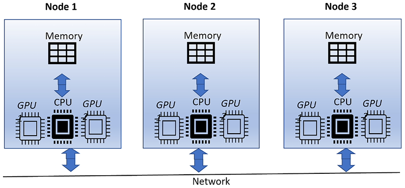
Figure 15.3: Hybrid strategy for multi-resource processing

As we explore the potential of parallel computing in running large-scale algorithms, it is equally important to understand the theoretical limitations that govern its efficiency.

In the following section, we will delve into the fundamental constraints of parallel computing, shedding light on the factors that influence its performance and the extent to which it can be optimized.

Understanding theoretical limitations of parallel computing

It is important to note that parallel algorithms are not a silver bullet. Even the best-designed parallel architectures may not give the performance that we may expect. The complexities of parallel computing, such as communication overhead and synchronization, make it challenging to achieve optimal efficiency. One law that has been developed to help navigate these complexities and better understand the potential gains and limitations of parallel algorithms is Amdahl’s law.

Amdahl’s law

Gene Amdahl was one of the first people to study parallel processing in the 1960s. He proposed Amdahl’s law, which is still applicable today and is a basis on which to understand the various trade-offs involved when designing a parallel computing solution. Amdahl’s law provides a theoretical limit on the maximum improvement in execution time that can be achieved with a parallelized version of an algorithm, given the proportion of the algorithm that can be parallelized.

It is based on the concept that in any computing process, not all processes can be executed in parallel. There will be a sequential portion of the process that cannot be parallelized.

Deriving Amdahl’s law

Consider an algorithm or task that can be divided into a parallelizable fraction (f) and a serial fraction (1 - f). The parallelizable fraction refers to the portion of the task that can be executed simultaneously across multiple resources or processors. These tasks don’t depend on each other and can be run in parallel, hence the term “parallelizable.” On the other hand, the serial fraction is part of the task that cannot be divided and must be executed in sequence, one after the other, hence “serial.”

Let Tp(1) represent the time required to process this task on a single processor. This can be expressed as:

T_p(1) = N(1 - f)τ_p + N(f)τ_p = Nτ_p

In these equations, N and τp denote:

• N: The total number of tasks or iterations that the algorithm or task must perform, consistent across both single and parallel processors.
• τ_p: The time taken by a processor to complete a single unit of work, task, or iteration, which remains constant regardless of the number of processors used.

The preceding equation calculates the total time taken to process all tasks on a single processor. Now, let’s examine a scenario where the task is executed on N parallel processors.

The time taken for this execution can be represented as T_p(N). In the following diagram, on the X-axis, we have Number of processors. This represents the number of computing units or cores used to execute our program. As we move right along the X-axis, we are increasing the number of processors used. The Y-axis represents Speedup. This is a measure of how much faster our program runs with multiple processors compared to using just one. As we move up the Y-axis, the speed of our program increases proportionally, resulting in more efficient task execution.

The graph in Figure 15.4 and Amdahl’s law show us that more processors can improve performance, but there’s a limit due to the sequential part of our code. This principle is a classic example of diminishing returns in parallel computing.

N = N(1 - f)τ_p + (f)τ_p

Here, the first term on the RHS (Right Hand Side) represents the time taken to process the serial part of the task, while the second term denotes the time taken to process the parallel part.

The speedup in this case is due to the distribution of the parallel part of the task over N processors. Amdahl’s law defines the speedup S(N) achieved by using N processors as:

For significant speedup, the following condition must be satisfied:

1 - f << f / N (4.4)

This inequality indicates that the parallel portion (f) must be very close to unity, especially when N is large.

Now, let’s look at a typical graph that explains Amdahl’s law:

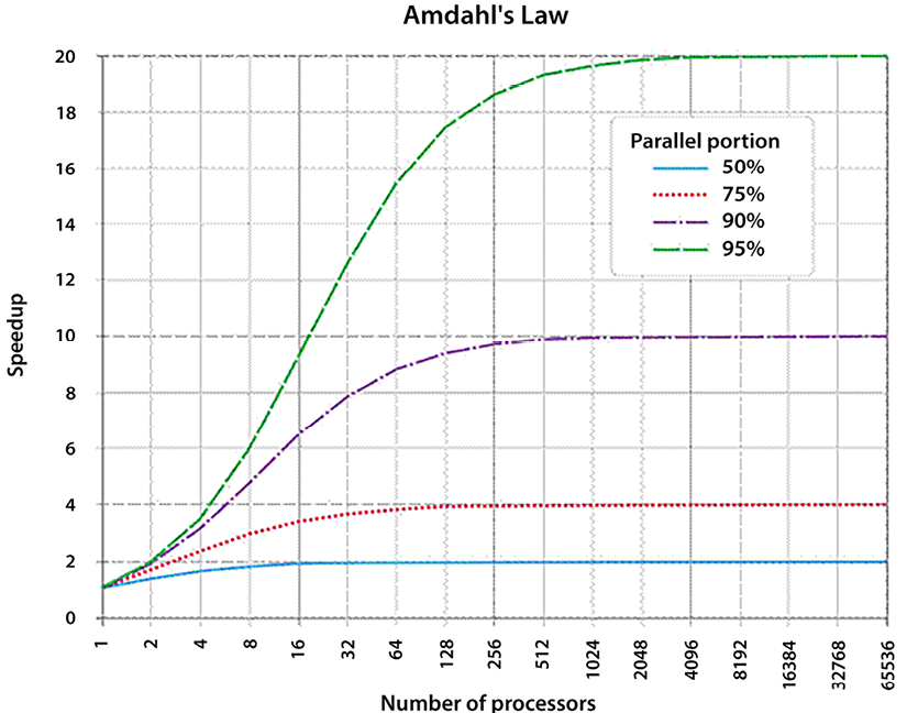
Figure 15.4: Diminishing returns in parallel processing: visualizing Amdahl’s law

In Figure 15.4, the X-axis represents the number of processors (N), corresponding to the computing units or cores used to execute the program. As we move to the right along the X-axis, N increases. The Y-axis denotes the speedup (S), a measure of the improvement in the program’s execution time T_p with multiple processors compared to using just one. Moving up the Y-axis indicates an increase in the program’s execution speed.

The graph features four lines, each representing the speedup S obtained from parallel processing for different percentages of the parallelizable fraction (f): 50%, 75%, 90%, and 95%:

• 50% parallel (f = 0.5): This line exhibits the smallest speedup S. Although more processors (N) are added, half of the program runs sequentially, limiting the speedup to a maximum of 2.
• 75% parallel (f = 0.75): The speedup S is higher compared to the 50% case. However, 25% of the program still runs sequentially, constraining the overall speedup.
• 90% parallel (f = 0.9): In this case, a significant speedup S is observed. Nevertheless, the sequential 10% of the program imposes a limit on the speedup.
• 95% parallel (f = 0.95): This line demonstrates the highest speedup S. Yet, the sequential 5% still imposes an upper limit on the speedup.

The graph, in conjunction with Amdahl’s law, highlights that while increasing the number of processors (N) can enhance performance, there exists an inherent limit due to the sequential part of the code (1 - f). This principle serves as a classic illustration of diminishing returns in parallel computing.

Amdahl’s law provides valuable insights into the potential performance gains achievable in multiprocessor systems and the importance of the parallelizable fraction (f) in determining the system’s overall speedup. After discussing the theoretical limitations of parallel computing, it is crucial to introduce and explore another powerful and widely-used parallel processing technology: the GPU and its associated programming framework, CUDA.

CUDA: Unleashing the potential of GPU architectures in parallel computing

GPUs were originally designed for graphics processing but have since evolved, exhibiting distinct characteristics that set them apart from CPUs and resulting in an entirely different computation paradigm.

Unlike CPUs, which have a limited number of cores, GPUs are composed of thousands of cores. It’s essential to recognize, however, that these cores, in isolation, are not as individually powerful as a CPU core. But, GPUs are quite efficient at executing numerous relatively simple computations in parallel.

As GPUs were originally designed for graphic processing, GPU architecture is ideal for graphic processing where multiple operations can be executed independently. For example, rendering an image involves the computation of color and brightness for each pixel in the image. These calculations are largely independent of each other and hence can be conducted simultaneously, leveraging the multi-core architecture of the GPU.

Bottom of form

This design choice allows GPUs to be extremely efficient at tasks they’re designed for, like rendering graphics and processing large datasets. Here is the architecture of GPUs shown in Figure 15.5:

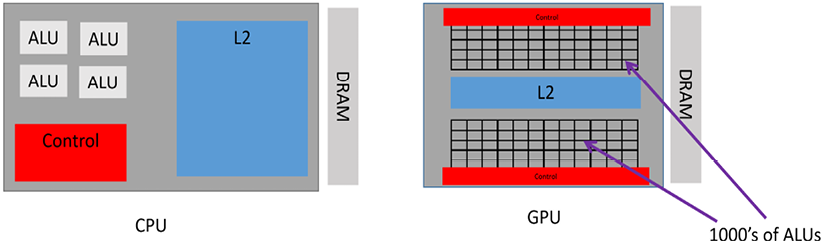
Figure 15.5: Architecture of GPUs

This unique architecture is not only beneficial for graphics processing but also significantly advantageous for other types of computational problems. Any problem that can be segmented into smaller, independent tasks can exploit this architecture for faster processing. This includes domains like scientific computing, machine learning, and even cryptocurrency mining, where massive datasets and complex computations are the norm.

Soon after GPUs became mainstream, data scientists started exploring them for their potential to efficiently perform parallel operations. As a typical GPU has thousands of Arithmetic Logic Units (ALUs), it has the potential to spawn thousands of concurrent processes. Note that the ALU is the workhorse of the core that performs most of the actual computations. This large number of ALUs makes GPUs well suited to tasks where the same operation needs to be performed on many data points simultaneously, such as vector and matrix operations common in data science and machine learning. Hence, algorithms that can perform parallel computations are best suited to GPUs. For example, an object search in a video is known to be at least 20 times faster in GPUs, compared to CPUs. Graph algorithms, which were discussed in Chapter 5, Graph Algorithms, are known to run much faster on GPUs than on CPUs.

In 2007, NVIDIA developed the open-source framework called Compute Unified Device Architecture (CUDA) to enable data scientists to harness the power of GPUs for their algorithms. CUDA abstracts the CPU and GPU as the host and the device, respectively.

Host refers to the CPU and main memory, responsible for executing the main program and offloading data-parallel computations to the GPU.

Device refers to the GPU and its memory (VRAM), responsible for executing kernels that perform data-parallel computations.

In a typical CUDA program, the host allocates memory on the device, transfers input data, and invokes a kernel. The device performs the computation, and the results are stored back in its memory. The host then retrieves the results. This division of labor leverages the strengths of each component, with the CPU handling complex logic and the GPU managing large-scale, data-parallel computations.

CUDA runs on NVIDIA GPUs and requires OS kernel support, initially starting with Linux and later extending to Windows. The CUDA Driver API bridges the programming language API and the CUDA driver, with support for C, C++, and Python.

Parallel processing in LLMs: A case study in Amdahl’s law and diminishing returns

LLMs, like ChatGPT, are intricate systems that generate text remarkably similar to human-written prose, given an initial prompt. This task involves a series of complex operations, which can be broadly divided into sequential and parallelizable tasks.

Sequential tasks are those that must occur in a specific order, one after the other. These tasks may include preprocessing steps like tokenizing, where the input text is broken down into smaller pieces, often words or phrases, which the model can understand. It may also encompass post-processing tasks like decoding, where the model’s output, often in the form of token probabilities, is translated back into human-readable text. These sequential tasks are critical to the function of the model, but by nature, they cannot be split up and run concurrently.

On the other hand, parallelizable tasks are those that can be broken down and run simultaneously. A key example of this is the forward propagation stage in the model’s neural network. Here, computations for each layer in the network can be performed concurrently. This operation constitutes the vast majority of the model’s computation time, and it is here where the power of parallel processing can be harnessed.

Now, assume that we’re working with a GPU that has 1,000 cores. In the context of language models, the parallelizable portion of the task might involve the forward propagation stage, where computations for each layer in the neural network can be performed concurrently. Let’s posit that this constitutes 95% of the total computation time. The remaining 5% of the task, which could involve operations like tokenizing and decoding, is sequential and cannot be parallelized.

Applying Amdahl’s law to this scenario gives us:

Speedup = 1 / ((1 - 0.95) + 0.95/1000) = 1 / (0.05 + 0.00095) = 19.61

Under ideal circumstances, this indicates that our language processing task could be completed about 19.61 times faster on a 1,000-core GPU than on a single-core CPU.

To further illustrate the diminishing returns of parallel computing, let’s adjust the number of cores to 2, 50, and 100:

• For 2 cores: Speedup = 1 / ((1 - 0.95) + 0.95/2) = 1.67
• For 50 cores: Speedup = 1 / ((1 - 0.95) + 0.95/50) = 14.71
• For 100 cores: Speedup = 1 / ((1 - 0.95) + 0.95/100) = 16.81

As seen from our calculations, adding more cores to a parallel computing setup doesn’t lead to an equivalent increase in speedup. This is a prime example of the concept of diminishing returns in parallel computing. Despite doubling the number of cores from 2 to 4, or increasing them 50-fold from 2 to 100, the speedup doesn’t double or increase 50 times. Instead, the speedup hits a theoretical limit as per Amdahl’s law.

The primary factor behind this diminishing return is the existence of a non-parallelizable portion in the task. In our case, operations like tokenizing and decoding form this sequential part, accounting for 5% of the total computation time. No matter how many cores we add to the system or how efficiently we can carry out the parallelizable part, this sequential portion places an upper limit on the achievable speedup. It will always be there, demanding its share of the computation time.

Amdahl’s law elegantly captures this characteristic of parallel computing. It states that the maximum potential speedup using parallel processing is dictated by the non-parallelizable part of the task. The law serves as a reminder to algorithm designers and system architects that while parallelism can dramatically speed up computation, it is not an infinite resource to be tapped for speed. It underscores the importance of identifying and optimizing the sequential components of an algorithm in order to maximize the benefits of parallel processing.

This understanding is particularly important in the context of LLMs, where the sheer scale of computations makes efficient resource utilization a key concern. It underlines the need for a balanced approach that combines parallel computing strategies with efforts to optimize the performance of the sequential parts of the task.

Rethinking data locality

Traditionally, in parallel and distributed processing, the data locality principle is pivotal in deciding the optimal resource allocation. It fundamentally suggests that the movement of data should be discouraged in distributed infrastructures. Whenever possible, instead of moving data, it should be processed locally on the node where it resides; otherwise, it reduces the benefit of parallelization and horizontal scaling, where horizontal scaling is the process of increasing a system’s capacity by adding more machines or nodes to distribute the workload, enabling it to handle higher amounts of traffic or data.

As networking bandwidth has improved over the years, the limitations imposed by data locality have become less significant. The increased data transfer speeds enable efficient communication between nodes in a distributed computing environment, reducing the reliance on data locality for performance optimization. The network bandwidth can be quantified by the network bisection bandwidth, which is the bandwidth between two equal parts of a network. This is important in distributed computing with resources that are physically distributed. If we draw a line somewhere between two sets of resources in a distributed network, the bisectional bandwidth is the rate of communication at which servers on one side of the line can communicate with servers on the other side, as shown in Figure 15.6. For distributed computing to work efficiently, this is the most important parameter to consider. If we do not have enough network bisection bandwidth, the benefits gained by the availability of multiple execution engines in distributed computing will be overshadowed by slow communication links.

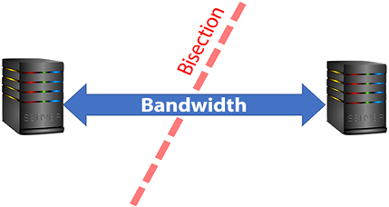
Figure 15.6: Bisection bandwidth

A high bisectional bandwidth enables us to process the data where it is without copying it. These days, major cloud computing providers offer exceptional bisection bandwidth. For example, within a Google data center, the bisection bandwidth is as high as 1 petabyte per second. Other major Cloud vendors offer similar bandwidth. In contrast, a typical enterprise network might only provide bisection bandwidth in the range of 1 to 10 gigabytes per second.

This vast difference in speed demonstrates the remarkable capabilities of modern Cloud infrastructure, making it well suited to large-scale data processing tasks.

The increased petabit bisectional bandwidth has opened up new options and design patterns for efficiently storing and processing big data. These new options include alternative methods and design patterns that have become viable due to the increased network capacity, enabling faster and more efficient data processing.

Benefiting from cluster computing using Apache Spark

Apache Spark is a widely used platform for managing and leveraging cluster computing. In this context, “cluster computing” involves grouping together several machines and making them work together as a single system to solve a problem. Spark doesn’t merely implement this; it creates and controls these clusters to achieve high-speed data processing.

Within Apache Spark, data undergoes a transformation into what’s known as Resilient Distributed Datasets (RDDs). These are effectively the backbone of Apache Spark’s data abstraction.

RDDs are immutable, meaning they can’t be altered once created, and are collections of elements that can be processed in parallel. In other words, different pieces of these datasets can be worked on at the same time, thereby accelerating data processing.

When we say “fault-tolerant,” we mean that RDDs have the ability to recover from potential failures or errors during execution. This makes them robust and reliable for big data processing tasks. They’re split into smaller chunks known as “partitions,” which are then distributed across various nodes or individual computers in the cluster. The size of these partitions can vary and is primarily determined by the nature of the task and the configuration of the Spark application.

Spark’s distributed computing framework allows the tasks to be distributed across multiple nodes, which can significantly improve processing speed and efficiency.

The Spark architecture is composed of several main components, including the driver program, executor, worker node, and cluster manager.

• Driver program: The driver program is a key component in a Spark application, functioning much like the control center of operations. It resides in its own separate process, often located on a machine known as the driver machine. The driver program’s role is like that of a conductor of an orchestra; it runs the primary Spark program and oversees the many tasks within it.

  Among the main tasks of the driver program are handling and running the SparkSession. The SparkSession is crucial to the Spark application as it wraps around the SparkContext. The SparkContext is like the central nervous system of the Spark application – it’s the gateway for the application to interact with the Spark computational ecosystem.

  To simplify, imagine the Spark application as an office building. The driver program is like the building manager, responsible for overall operation and maintenance. Within this building, the SparkSession represents an individual office, and the SparkContext is the main entrance to that office. The essence is that these components – the driver program, SparkSession, and SparkContext – work together to coordinate tasks and manage resources within a Spark application. The SparkContext is packed with fundamental functions and context information that is pre-loaded at the start time of the application. Moreover, it carries vital details about the cluster, such as its configuration and status, which are crucial for the application to run and execute tasks effectively.

• Cluster manager: The driver program interacts seamlessly with the cluster manager. The cluster manager is an external service that provides and manages resources across the cluster, such as computing power and memory. The driver program and the cluster manager work hand in hand to identify available resources in the cluster, allocate them effectively, and manage their usage throughout the life cycle of the Spark application.
• Executors: An executor refers to a dedicated computational process that is spawned specifically for an individual Spark application running on a node within a cluster. Each of these executor processes operates on a worker node, effectively acting as the computational “muscle” behind your Spark application.
• The sharing of both memory and global parameters in this way can significantly enhance the speed and efficiency of task execution, making Spark a highly performant framework for big data processing.
• Worker node: A worker node, true to its name, is charged with carrying out the actual execution of tasks within the distributed Spark system.

  Each worker node is capable of hosting multiple executors, which in turn can serve numerous Spark applications:

  

  Figure 15.7: Spark’s distributed architecture

How Apache Spark empowers large-scale algorithm processing

Apache Spark has emerged as a leading platform for processing and analyzing big data, thanks to its powerful distributed computing capabilities, fault-tolerant nature, and ease of use. In this section, we will explore how Apache Spark empowers large-scale algorithm processing, making it an ideal choice for complex, resource-intensive tasks.

Distributed computing

At the core of Apache Spark’s architecture is the concept of data partitioning, which allows data to be divided across multiple nodes in a cluster. This feature enables parallel processing and efficient resource utilization, both of which are crucial for running large-scale algorithms. Spark’s architecture comprises a driver program and multiple executor processes distributed across worker nodes. The driver program is responsible for managing and distributing tasks across the executors, while each executor runs multiple tasks concurrently in separate threads, allowing for high throughput.

In-memory processing

One of Spark’s standout features is its in-memory processing capability. Unlike traditional disk-based systems, Spark can cache intermediate data in memory, significantly speeding up iterative algorithms that require multiple passes over the data.

• This in-memory processing capability is particularly beneficial for large-scale algorithms, as it minimizes the time spent on disk I/O, leading to faster computation times and more efficient use of resources.

Using large-scale algorithms in cloud computing

The rapid growth of data and the increasing complexity of machine learning models have made distributed model training an essential component of modern deep learning pipelines. Large-scale algorithms demand vast amounts of computational resources and necessitate efficient parallelism to optimize their training times. Cloud computing offers an array of services and tools that facilitate distributed model training, allowing you to harness the full potential of resource-hungry, large-scale algorithms.

Some of the key advantages of using the Cloud for distributed model training include:

• Scalability: The Cloud provides virtually unlimited resources, allowing you to scale your model training workloads to meet the demands of large-scale algorithms.
• Flexibility: The Cloud supports a wide range of machine learning frameworks and libraries, enabling you to choose the most suitable tools for your specific needs.
• Cost-effectiveness: With the Cloud, you can optimize your training costs by selecting the right instance types and leveraging spot instances to reduce expenses.

Example

As we delve deeper into machine learning models, especially those dealing with Natural Language Processing (NLP) tasks, we notice an increasing need for computational resources. For instance, transformers like GPT-3 for large-scale language modeling tasks can have billions of parameters, demanding substantial processing power and memory. Training such models on colossal datasets, such as Common Crawl, which contains billions of web pages, further escalates these requirements.

Cloud computing emerges as a potent solution here. It offers services and tools for distributed model training, enabling us to access an almost infinite pool of resources, scale our workloads, and select the most suitable machine learning frameworks. What’s more, cloud computing facilitates cost optimization by providing flexible instance types and spot instances – essentially bidding for spare computing capacity. By delegating these resource-heavy tasks to the cloud, we can concentrate more on innovative work, speeding up the training process, and developing more powerful models.

Summary

In this chapter, we examined the concepts and principles of large-scale and parallel algorithm design. The pivotal role of parallel computing was analyzed, with particular emphasis on its capacity to effectively distribute computational tasks across multiple processing units. The extraordinary capabilities of GPUs were studied in detail, illustrating their utility in executing numerous threads concurrently. Moreover, we discussed distributed computing platforms, specifically Apache Spark and cloud computing environments. Their importance in facilitating the development and deployment of large-scale algorithms was underscored, providing a robust, scalable, and cost-effective infrastructure for high-performance computations.

Learn more on Discord

To join the Discord community for this book – where you can share feedback, ask questions to the author, and learn about new releases – follow the QR code below:

https://packt.link/WHLel