1

Overview of Algorithms

An algorithm must be seen to be believed.

– Donald Knuth

This book covers the information needed to understand, classify, select, and implement important algorithms. In addition to explaining their logic, this book also discusses data structures, development environments, and production environments that are suitable for different classes of algorithms. This is the second edition of this book. In this edition, we especially focus on modern machine learning algorithms that are becoming more and more important. Along with the logic, practical examples of the use of algorithms to solve actual everyday problems are also presented.

This chapter provides an insight into the fundamentals of algorithms. It starts with a section on the basic concepts needed to understand the workings of different algorithms. To provide a historical perspective, this section summarizes how people started using algorithms to mathematically formulate a certain class of problems. It also mentions the limitations of different algorithms. The next section explains the various ways to specify the logic of an algorithm. As Python is used in this book to write the algorithms, how to set up a Python environment to run the examples is explained. Then, the various ways that an algorithm’s performance can be quantified and compared against other algorithms are discussed. Finally, this chapter discusses various ways a particular implementation of an algorithm can be validated.

To sum up, this chapter covers the following main points:

• What is an algorithm?
• The phases of an algorithm
• Development environment
• Algorithm design techniques
• Performance analysis
• Validating an algorithm

What is an algorithm?

In the simplest terms, an algorithm is a set of rules for carrying out some calculations to solve a problem. It is designed to yield results for any valid input according to precisely defined instructions. If you look up the word algorithm in a dictionary (such as American Heritage), it defines the concept as follows:

An algorithm is a finite set of unambiguous instructions that, given some set of initial conditions, can be performed in a prescribed sequence to achieve a certain goal and that has a recognizable set of end conditions.

Designing an algorithm is an effort to create a mathematical recipe in the most efficient way that can effectively be used to solve a real-world problem. This recipe may be used as the basis for developing a more reusable and generic mathematical solution that can be applied to a wider set of similar problems.

The phases of an algorithm

The different phases of developing, deploying, and finally, using an algorithm are illustrated in Figure 1.1:

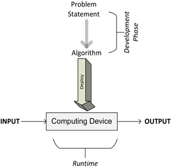
Figure 1.1: The different phases of developing, deploying, and using an algorithm

As we can see, the process starts with understanding the requirements from the problem statement that details what needs to be done. Once the problem is clearly stated, it leads us to the development phase.

The development phase consists of two phases:

1. The design phase: In the design phase, the architecture, logic, and implementation details of the algorithm are envisioned and documented. While designing an algorithm, we keep both accuracy and performance in mind. While searching for the best solution to a given problem, in many cases, we will end up having more than one candidate algorithm. The design phase of an algorithm is an iterative process that involves comparing different candidate algorithms. Some algorithms may provide simple and fast solutions but may compromise accuracy. Other algorithms may be very accurate but may take considerable time to run due to their complexity. Some of these complex algorithms may be more efficient than others. Before making a choice, all the inherent tradeoffs of the candidate algorithms should be carefully studied. Particularly for a complex problem, designing an efficient algorithm is important. A correctly designed algorithm will result in an efficient solution that will be capable of providing both satisfactory performance and reasonable accuracy at the same time.
2. The coding phase: In the coding phase, the designed algorithm is converted into a computer program. It is important that the computer program implements all the logic and architecture suggested in the design phase.

The requirements of the business problem can be divided into functional and non-functional requirements. The requirements that directly specify the expected features of the solutions are called the functional requirements. Functional requirements detail the expected behavior of the solution. On the other hand, the non-functional requirements are about the performance, scalability, usability, and accuracy of the algorithm. Non-functional requirements also establish the expectations about the security of the data. For example, let us consider that we are required to design an algorithm for a credit card company that can identify and flag fraudulent transactions. Function requirements in this example will specify the expected behavior of a valid solution by providing the details of the expected output given a certain set of input data. In this case, the input data may be the details of the transaction, and the output may be a binary flag that labels a transaction as fraudulent or non-fraudulent. In this example, the non-functional requirements may specify the response time of each of the predictions. Non-functional requirements will also set the allowable thresholds for accuracy. As we are dealing with financial data in this example, the security requirements related to user authentication, authorization, and data confidentiality are also expected to be part of non-functional requirements.

Note that functional and non-functional requirements aim to precisely define what needs to be done. Designing the solution is about figuring out how it will be done. And implementing the design is developing the actual solution in the programming language of your choice. Coming up with a design that fully meets both functional and non-functional requirements may take lots of time and effort. The choice of the right programming language and development/production environment may depend on the requirements of the problem. For example, as C/C++ is a lower-level language than Python, it may be a better choice for algorithms needing compiled code and lower-level optimization.

Once the design phase is completed and the coding is complete, the algorithm is ready to be deployed. Deploying an algorithm involves the design of the actual production environment in which the code will run. The production environment needs to be designed according to the data and processing needs of the algorithm. For example, for parallelizable algorithms, a cluster with an appropriate number of computer nodes will be needed for the efficient execution of the algorithm. For data-intensive algorithms, a data ingress pipeline and the strategy to cache and store data may need to be designed. Designing a production environment is discussed in more detail in Chapter 15, Large-Scale Algorithms, and Chapter 16, Practical Considerations.

Once the production environment is designed and implemented, the algorithm is deployed, which takes the input data, processes it, and generates the output as per the requirements.

Development environment

Once designed, algorithms need to be implemented in a programming language as per the design. For this book, we have chosen the programming language Python. We chose it because Python is flexible and is an open-source programming language. Python is also one of the languages that you can use in various cloud computing infrastructures, such as Amazon Web Services (AWS), Microsoft Azure, and Google Cloud Platform (GCP).

The official Python home page is available at https://www.python.org/, which also has instructions for installation and a useful beginner’s guide.

A basic understanding of Python is required to better understand the concepts presented in this book.

For this book, we expect you to use the most recent version of Python 3. At the time of writing, the most recent version is 3.10, which is what we will use to run the exercises in this book.

We will be using Python throughout this book. We will also be using Jupyter Notebook to run the code. The rest of the chapters in this book assume that Python is installed and Jupyter Notebook has been properly configured and is running.

Python packages

Python is a general-purpose language. It follows the philosophy of “batteries included,” which means that there is a standard library that is available, without making the user download separate packages. However, the standard library modules only provide the bare minimum functionality. Based on the specific use case you are working on, additional packages may need to be installed. The official third-party repository for Python packages is called PyPI, which stands for Python Package Index. It hosts Python packages both as source distribution and pre-compiled code. Currently, there are more than 113,000 Python packages hosted at PyPI. The easiest way to install additional packages is through the pip package management system. pip is a nerdy recursive acronym, which are abundant in Python culture. pip stands for Pip Installs Python. The good news is that starting from version 3.4 of Python, pip is installed by default. To check the version of pip, you can type on the command line:

pip --version

This pip command can be used to install additional packages:

pip install PackageName

The packages that have already been installed need to be periodically updated to get the latest functionality. This is achieved by using the upgrade flag:

pip install PackageName --upgrade

And to install a specific version of a Python package:

pip install PackageName==2.1

pip install -r requirements.txt

Now let us look into the main packages that we will be using in this book.

The SciPy ecosystem

Scientific Python (SciPy)—pronounced sigh pie—is a group of Python packages created for the scientific community. It contains many functions, including a wide range of random number generators, linear algebra routines, and optimizers.

SciPy is a comprehensive package and, over time, people have developed many extensions to customize and extend the package according to their needs. SciPy is performant as it acts as a thin wrapper around optimized code written in C/C++ or Fortran.

The following are the main packages that are part of this ecosystem:

• NumPy: For algorithms, the ability to create multi-dimensional data structures, such as arrays and matrices, is really important. NumPy offers a set of array and matrix data types that are important for statistics and data analysis. Details about NumPy can be found at http://www.numpy.org/.
• scikit-learn: This machine learning extension is one of the most popular extensions of SciPy. Scikit-learn provides a wide range of important machine learning algorithms, including classification, regression, clustering, and model validation. You can find more details about scikit-learn at http://scikit-learn.org/.
• pandas: pandas contains the tabular complex data structure that is used widely to input, output, and process tabular data in various algorithms. The pandas library contains many useful functions and it also offers highly optimized performance. More details about pandas can be found at http://pandas.pydata.org/.
• Matplotlib: Matplotlib provides tools to create powerful visualizations. Data can be presented as line plots, scatter plots, bar charts, histograms, pie charts, and so on. More information can be found at https://matplotlib.org/.

Using Jupyter Notebook

We will be using Jupyter Notebook and Google’s Colaboratory as the IDE. More details about the setup and the use of Jupyter Notebook and Colab can be found in Appendix A and B.

Algorithm design techniques

An algorithm is a mathematical solution to a real-world problem. When designing an algorithm, we keep the following three design concerns in mind as we work on designing and fine-tuning the algorithms:

• Concern 1: Is this algorithm producing the result we expected?
• Concern 2: Is this the most optimal way to get these results?
• Concern 3: How is the algorithm going to perform on larger datasets?

It is important to understand the complexity of the problem itself before designing a solution for it. For example, it helps us to design an appropriate solution if we characterize the problem in terms of its needs and complexity.

Generally, the algorithms can be divided into the following types based on the characteristics of the problem:

• Data-intensive algorithms: Data-intensive algorithms are designed to deal with a large amount of data. They are expected to have relatively simplistic processing requirements. A compression algorithm applied to a huge file is a good example of data-intensive algorithms. For such algorithms, the size of the data is expected to be much larger than the memory of the processing engine (a single node or cluster), and an iterative processing design may need to be developed to efficiently process the data according to the requirements.
• Compute-intensive algorithms: Compute-intensive algorithms have considerable processing requirements but do not involve large amounts of data. A simple example is the algorithm to find a very large prime number. Finding a strategy to divide the algorithm into different phases so that at least some of the phases are parallelized is key to maximizing the performance of the algorithm.
• Both data and compute-intensive algorithms: There are certain algorithms that deal with a large amount of data and also have considerable computing requirements. Algorithms used to perform sentiment analysis on live video feeds are a good example of where both the data and the processing requirements are huge in accomplishing the task. Such algorithms are the most resource-intensive algorithms and require careful design of the algorithm and intelligent allocation of available resources.

To characterize the problem in terms of its complexity and needs, it helps if we study its data and compute dimensions in more depth, which we will do in the following section.

The data dimension

To categorize the data dimension of the problem, we look at its volume, velocity, and variety (the 3Vs), which are defined as follows:

• Volume: The volume is the expected size of the data that the algorithm will process.
• Velocity: The velocity is the expected rate of new data generation when the algorithm is used. It can be zero.
• Variety: The variety quantifies how many different types of data the designed algorithm is expected to deal with.

Figure 1.2 shows the 3Vs of the data in more detail. The center of this diagram shows the simplest possible data, with a small volume and low variety and velocity. As we move away from the center, the complexity of the data increases. It can increase in one or more of the three dimensions.

For example, in the dimension of velocity, we have the batch process as the simplest, followed by the periodic process, and then the near real-time process. Finally, we have the real-time process, which is the most complex to handle in the context of data velocity. For example, a collection of live video feeds gathered by a group of monitoring cameras will have a high volume, high velocity, and high variety and may need an appropriate design to have the ability to store and process data effectively:

Figure 1.2: 3Vs of Data: Volume, Velocity, and Variety

Let us consider three examples of use cases having three different types of data:

• First, consider a simple data-processing use case where the input data is a .csv file. In this case, the volume, velocity, and variety of the data will be low.
• Second, consider the use case where the input data is the live stream of a security video camera. Now the volume, velocity, and variety of the data will be quite high and should be kept in mind while designing an algorithm for it.
• Third, consider the use case of a typical sensor network. Let us assume that the data source of the sensor network is a mesh of temperature sensors installed in a large building. Although the velocity of the data being generated is typically very high (as new data is being generated very quickly), the volume is expected to be quite low (as each data element is typically only 16-bits long consisting of an 8-bit measurement plus 8-bit metadata such as a timestamp and the geo-coordinates.

The processing requirements, storage needs, and suitable software stack selection will be different for all the above three examples and, in general, are dependent on the volume, velocity, and variety of the data sources. It is important to first characterize data as the first step of designing an algorithm.

The compute dimension

To characterize the compute dimension, we analyze the processing needs of the problem at hand. The processing needs of an algorithm determine what sort of design is most efficient for it. For example, complex algorithms, in general, require lots of processing power. For such algorithms, it may be important to have multi-node parallel architecture. Modern deep algorithms usually involve considerable numeric processing and may need the power of GPUs or TUPs as discussed in Chapter 16, Practical Considerations.

Performance analysis

Analyzing the performance of an algorithm is an important part of its design. One of the ways to estimate the performance of an algorithm is to analyze its complexity.

Complexity theory is the study of how complicated algorithms are. To be useful, any algorithm should have three key features:

• Should be correct: A good algorithm should produce the correct result. To confirm that an algorithm is working correctly, it needs to be extensively tested, especially testing edge cases.
• Should be understandable: A good algorithm should be understandable. The best algorithm in the world is not very useful if it’s too complicated for us to implement on a computer.
• Should be efficient: A good algorithm should be efficient. Even if an algorithm produces the correct result, it won’t help us much if it takes a thousand years or if it requires 1 billion terabytes of memory.

There are two possible types of analysis to quantify the complexity of an algorithm:

• Space complexity analysis: Estimates the runtime memory requirements needed to execute the algorithm.
• Time complexity analysis: Estimates the time the algorithm will take to run.

Let us study them one by one:

Space complexity analysis

Space complexity analysis estimates the amount of memory required by the algorithm to process input data. While processing the input data, the algorithm needs to store the transient temporary data structures in memory. The way the algorithm is designed affects the number, type, and size of these data structures. In an age of distributed computing and with increasingly large amounts of data that needs to be processed, space complexity analysis is becoming more and more important. The size, type, and number of these data structures will dictate the memory requirements for the underlying hardware. Modern in-memory data structures used in distributed computing need to have efficient resource allocation mechanisms that are aware of the memory requirements at different execution phases of the algorithm. Complex algorithms tend to be iterative in nature. Instead of bringing all the information into the memory at once, such algorithms iteratively populate the data structures. To calculate the space complexity, it is important to first classify the type of iterative algorithm we plan to use. An iterative algorithm can use one of the following three types of iterations:

• Converging Iterations: As the algorithm proceeds through iterations, the amount of data it processes in each individual iteration decreases. In other words, space complexity decreases as the algorithm proceeds through its iterations. The main challenge is to tackle the space complexity of the initial iterations. Modern scalable cloud infrastructures such as AWS and Google Cloud are best suited to run such algorithms.
• Diverging Iterations: As the algorithm proceeds through iterations, the amount of data it processes in each individual iteration increases. As the space complexity increases with the algorithm’s progress through iterations, it is important to set constraints to prevent the system from becoming unstable. The constraints can be set by limiting the number of iterations and/or by setting a limit on the size of initial data.
• Flat Iterations: As the algorithm proceeds through iterations, the amount of data it processes in each individual iteration remains constant. As space complexity does not change, elasticity in infrastructure is not needed.

To calculate the space complexity, we need to focus on one of the most complex iterations. In many algorithms, as we converge towards the solution, the resource needs are gradually reduced. In such cases, initial iterations are the most complex and give us a better estimate of space complexity. Once chosen, we estimate the total amount of memory used by the algorithm, including the memory used by its transient data structures, execution, and input values. This will give us a good estimate of the space complexity of an algorithm.

The following are guidelines to minimize the space complexity:

• Whenever possible, try to design an algorithm as iterative.
• While designing an iterative algorithm, whenever there is a choice, prefer a larger number of iterations over a smaller number of iterations. A fine-grained larger number of iterations is expected to have less space complexity.
• Algorithms should bring only the information needed for current processing into memory. Whatever is not needed should be flushed out from the memory.

Space complexity analysis is a must for the efficient design of algorithms. If proper space complexity analysis is not conducted while designing a particular algorithm, insufficient memory availability for the transient temporary data structures may trigger unnecessary disk spillovers, which could potentially considerably affect the performance and efficiency of the algorithm.

In this chapter, we will look deeper into time complexity. Space complexity will be discussed in Chapter 15, Large-Scale Algorithms, in more detail, where we will deal with large-scale distributed algorithms with complex runtime memory requirements.

Time complexity analysis

Time complexity analysis estimates how long it will take for an algorithm to complete its assigned job based on its structure. In contrast to space complexity, time complexity is not dependent on any hardware that the algorithm will run on. Time complexity analysis solely depends on the structure of the algorithm itself. The overall goal of time complexity analysis is to try to answer these important two questions:

• Will this algorithm scale? A well-designed algorithm should be fully capable of taking advantage of the modern elastic infrastructure available in cloud computing environments. An algorithm should be designed in a way such that it can utilize the availability of more CPUs, processing cores, GPUs, and memory. For example, an algorithm used for training a model in a machine learning problem should be able to use distributed training as more CPUs are available.

Such algorithms should also take advantage of GPUs and additional memory if made available during the execution of the algorithm.

• How well will this algorithm handle larger datasets?

To answer these questions, we need to determine the effect on the performance of an algorithm as the size of the data is increased and make sure that the algorithm is designed in a way that not only makes it accurate but also scales well. The performance of an algorithm is becoming more and more important for larger datasets in today’s world of “big data.”

In many cases, we may have more than one approach available to design the algorithm. The goal of conducting time complexity analysis, in this case, will be as follows:

“Given a certain problem and more than one algorithm, which one is the most efficient to use in terms of time efficiency?”

There can be two basic approaches to calculating the time complexity of an algorithm:

• A post-implementation profiling approach: In this approach, different candidate algorithms are implemented, and their performance is compared.
• A pre-implementation theoretical approach: In this approach, the performance of each algorithm is approximated mathematically before running an algorithm.

The advantage of the theoretical approach is that it only depends on the structure of the algorithm itself. It does not depend on the actual hardware that will be used to run the algorithm, the choice of the software stack chosen at runtime, or the programming language used to implement the algorithm.

Estimating the performance

The performance of a typical algorithm will depend on the type of data given to it as an input. For example, if the data is already sorted according to the context of the problem we are trying to solve, the algorithm may perform blazingly fast. If the sorted input is used to benchmark this particular algorithm, then it will give an unrealistically good performance number, which will not be a true reflection of its real performance in most scenarios. To handle this dependency of algorithms on the input data, we have different types of cases to consider when conducting a performance analysis.

The best case

In the best case, the data given as input is organized in a way that the algorithm will give its best performance. Best-case analysis gives the upper bound of the performance.

The worst case

The second way to estimate the performance of an algorithm is to try to find the maximum possible time it will take to get the job done under a given set of conditions. This worst-case analysis of an algorithm is quite useful as we are guaranteeing that regardless of the conditions, the performance of the algorithm will always be better than the numbers that come out of our analysis. Worst-case analysis is especially useful for estimating the performance when dealing with complex problems with larger datasets. Worst-case analysis gives the lower bound of the performance of the algorithm.

The average case

This starts by dividing the various possible inputs into various groups. Then, it conducts the performance analysis from one of the representative inputs from each group. Finally, it calculates the average of the performance of each of the groups.

Average-case analysis is not always accurate as it needs to consider all the different combinations and possibilities of input to the algorithm, which is not always easy to do.

Big O notation

Big O notation was first introduced by Bachmann in 1894 in a research paper to approximate an algorithm’s growth. He wrote:

“… with the symbol O(n) we express a magnitude whose order in respect to n does not exceed the order of n” (Bachmann 1894, p. 401).

Big-O notation provides a way to describe the long-term growth rate of an algorithm’s performance. In simpler terms, it tells us how the runtime of an algorithm increases as the input size grows. Let’s break it down with the help of two functions, f(n) and g(n). If we say f = O(g), what we mean is that as n approaches infinity, the ratio stays limited or bounded. In other words, no matter how large our input gets, f(n) will not grow disproportionately faster than g(n).

Let’s look at particular functions:

f(n) = 1000n² + 100n + 10

and

g(n) = n²

Note that both functions will approach infinity as n approaches infinity. Let’s find out if f = O(g) by applying the definition.

First, let us calculate ,

which will be equal to = = (1000 + ).

It is clear that is bounded and will not approach infinity as n approaches infinity.

Thus f(n) = O(g) = O(n²).

(n²) represents that the complexity of this function increases as the square of input n. If we double the number of input elements, the complexity is expected to increase by 4.

Note the following 4 rules when dealing with Big-O notation.

Rule 1:

Let us look into the complexity of loops in algorithms. If an algorithm performs a certain sequence of steps n times, then it has O(n) performance.

Rule 2:

Let us look into the nested loops of the algorithms. If an algorithm performs a function that has a loop of n¹ steps, and for each loop it performs another n² steps, the algorithm’s total performance is O(n¹ × n²).

For example, if an algorithm has both outer and inner loops having n steps, then the complexity of the algorithm will be represented by:

O(n*n) = O(n²)

Rule 3:

If an algorithm performs a function f(n) that takes n¹ steps and then performs another function g(n) that takes n² steps, the algorithm’s total performance is O(f(n)+g(n)).

Rule 4:

If an algorithm takes O(g(n) + h(n)) and the function g(n) is greater than h(n) for large n, the algorithm’s performance can be simplified to O(g(n)).

It means that O(1+n) = O(n).

And O(n²+ n³) = O(n²).

Rule 5:

When calculating the complexity of an algorithm, ignore constant multiples. If k is a constant, O(kf(n)) is the same as O(f(n)).

Also, O(f(k × n)) is the same as O(f(n)).

Thus O(5n²) = O(n²).

And O((3n²)) = O(n²).

Note that:

• The complexity quantified by Big O notation is only an estimate.
• For smaller sizes of data, we do not care about the time complexity. n⁰ in the graph defines the threshold above which we are interested in finding the time complexity. The shaded area describes this area of interest where we will analyze the time complexity.
• T(n) time complexity is more than the original function. A good choice of T(n) will try to create a tight upper bound for F(n).

The following table summarizes the different kinds of Big O notation types discussed in this section:

Constant time (O(1)) complexity

If an algorithm takes the same amount of time to run, independent of the size of the input data, it is said to run in constant time. It is represented by O(1). Let’s take the example of accessing the n^th element of an array. Regardless of the size of the array, it will take constant time to get the results. For example, the following function will return the first element of the array and has a complexity of O(1):

def get_first(my_list):
    return my_list[0]
get_first([1, 2, 3])

1

get_first([1, 2, 3, 4, 5, 6, 7, 8, 9, 10])

1

Note that:

• The addition of a new element to a stack is done by using push and removing an element from a stack is done by using pop. Regardless of the size of the stack, it will take the same time to add or remove an element.
• When accessing the element of the hashtable, note that it is a data structure that stores data in an associative format, usually as key-value pairs.

Linear time (O(n)) complexity

An algorithm is said to have a complexity of linear time, represented by O(n), if the execution time is directly proportional to the size of the input. A simple example is to add the elements in a single-dimensional data structure:

def get_sum(my_list):
    sum = 0
    for item in my_list:
        sum = sum + item
    return sum

Note the main loop of the algorithm. The number of iterations in the main loop increases linearly with an increasing value of n, producing an O(n) complexity in the following figure:

get_sum([1, 2, 3])

6

get_sum([1, 2, 3, 4])

10

Some other examples of array operations are as follows:

• Searching an element
• Finding the minimum value among all the elements of an array

Quadratic time (O(n2)) complexity

An algorithm is said to run in quadratic time if the execution time of an algorithm is proportional to the square of the input size; for example, a simple function that sums up a two-dimensional array, as follows:

def get_sum(my_list):
    sum = 0
    for row in my_list:
        for item in row:
            sum += item
    return sum

Note the nested inner loop within the other main loop. This nested loop gives the preceding code the complexity of O(n²):

get_sum([[1, 2], [3, 4]])

10

get_sum([[1, 2, 3], [4, 5, 6]])

21

Another example is the bubble sort algorithm (which will be discussed in Chapter 2, Data Structures Used in Algorithms).

Logarithmic time (O(logn)) complexity

An algorithm is said to run in logarithmic time if the execution time of the algorithm is proportional to the logarithm of the input size. With each iteration, the input size decreases by constant multiple factors. An example of a logarithmic algorithm is binary search. The binary search algorithm is used to find a particular element in a one-dimensional data structure, such as a Python list. The elements within the data structure need to be sorted in descending order. The binary search algorithm is implemented in a function named search_binary, as follows:

def search_binary(my_list, item):
    first = 0
    last = len(my_list)-1
    found_flag = False
    while(first <= last and not found_flag):
        mid = (first + last)//2
        if my_list[mid] == item:
            found_flag = True           
        else:
            if item < my_list[mid]:
                last = mid - 1
            else:
                first = mid + 1
    return found_flag
searchBinary([8,9,10,100,1000,2000,3000], 10)

True

searchBinary([8,9,10,100,1000,2000,3000], 5)

False

The main loop takes advantage of the fact that the list is ordered. It divides the list in half with each iteration until it gets to the result.

After defining the function, it is tested to search a particular element in lines 11 and 12. The binary search algorithm is further discussed in Chapter 3, Sorting and Searching Algorithms.

Note that among the four types of Big O notation types presented, O(n²) has the worst performance and O(logn) has the best performance. On the other hand, O(n²) is not as bad as O(n³), but still, algorithms that fall in this class cannot be used on big data as the time complexity puts limitations on how much data they can realistically process. The performance of four types of Big O notations is shown in Figure 1.3:

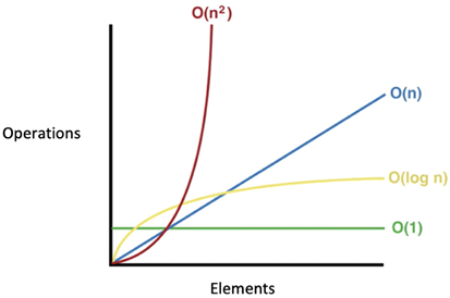
Figure 1.3: Big O complexity chart

One way to reduce the complexity of an algorithm is to compromise on its accuracy, producing a type of algorithm called an approximate algorithm.

Selecting an algorithm

How do you know which one is a better solution? How do you know which algorithm runs faster? Analyzing the time complexity of an algorithm may answer these types of questions.

To see where it can be useful, let’s take a simple example where the objective is to sort a list of numbers. There are a bunch of algorithms readily available that can do the job. The issue is how to choose the right one.

First, an observation that can be made is that if there are not too many numbers in the list, then it does not matter which algorithm we choose to sort the list of numbers. So, if there are only 10 numbers in the list (n=10), then it does not matter which algorithm we choose as it would probably not take more than a few microseconds, even with a very simple algorithm. But as n increases, the choice of the right algorithm starts to make a difference. A poorly designed algorithm may take a couple of hours to run, while a well-designed algorithm may finish sorting the list in a couple of seconds. So, for larger input datasets, it makes a lot of sense to invest time and effort, perform a performance analysis, and choose the correctly designed algorithm that will do the job required in an efficient manner.

Validating an algorithm

Validating an algorithm confirms that it is actually providing a mathematical solution to the problem we are trying to solve. A validation process should check the results for as many possible values and types of input values as possible.

Exact, approximate, and randomized algorithms

Validating an algorithm also depends on the type of the algorithm as the testing techniques are different. Let’s first differentiate between deterministic and randomized algorithms.

For deterministic algorithms, a particular input always generates exactly the same output. But for certain classes of algorithms, a sequence of random numbers is also taken as input, which makes the output different each time the algorithm is run. The k-means clustering algorithm, which is detailed in Chapter 6, Unsupervised Machine Learning Algorithms, is an example of such an algorithm:

Figure 1.4: Deterministic and Randomized Algorithms

Algorithms can also be divided into the following two types based on assumptions or approximation used to simplify the logic to make them run faster:

• An exact algorithm: Exact algorithms are expected to produce a precise solution without introducing any assumptions or approximations.
• An approximate algorithm: When the problem complexity is too much to handle for the given resources, we simplify our problem by making some assumptions. The algorithms based on these simplifications or assumptions are called approximate algorithms, which don’t quite give us the precise solution.

Let’s look at an example to understand the difference between exact and approximate algorithms—the famous traveling salesman problem, which was presented in 1930. Traveling salesman challenges you to find the shortest route for a particular salesman that visits each city (from a list of cities) and then returns to the origin, which is why he is named the traveling salesman. The first attempt to provide the solution will include generating all the permutations of cities and choosing the combination of cities that is cheapest. It is obvious that time complexity starts to become unmanageable beyond 30 cities.

If the number of cities is more than 30, one way of reducing the complexity is to introduce some approximations and assumptions.

For approximate algorithms, it is important to set the expectations for accuracy when gathering the requirements. Validating an approximation algorithm is about verifying that the error of the results is within an acceptable range.

Explainability

When algorithms are used for critical cases, it becomes important to have the ability to explain the reason behind each and every result whenever needed. This is necessary to make sure that decisions based on the results of the algorithms do not introduce bias.

The ability to exactly identify the features that are used directly or indirectly to come up with a particular decision is called the explainability of an algorithm. Algorithms, when used for critical use cases, need to be evaluated for bias and prejudice. The ethical analysis of algorithms has become a standard part of the validation process for those algorithms that can affect decision-making that relates to the lives of people.

For algorithms that deal with deep learning, explainability is difficult to achieve. For example, if an algorithm is used to refuse the mortgage application of a person, it is important to have the transparency and ability to explain the reason.

Algorithmic explainability is an active area of research. One of the effective techniques that have been recently developed is Local Interpretable Model-Agnostic Explanations (LIME), as proposed in the proceedings of the 22^nd Association for Computing Machinery (ACM) at the Special Interest Group on Knowledge Discovery and Data Mining (SIGKDD) international conference on knowledge discovery and data mining in 2016. LIME is based on a concept where small changes are introduced to the input for each instance and then an effort to map the local decision boundary for that instance is made. It can then quantify the influence of each variable for that instance.

Summary

This chapter was about learning the basics of algorithms. First, we learned about the different phases of developing an algorithm. We discussed the different ways of specifying the logic of an algorithm that are necessary for designing it. Then, we looked at how to design an algorithm. We learned two different ways of analyzing the performance of an algorithm. Finally, we studied different aspects of validating an algorithm.

After going through this chapter, we should be able to understand the pseudocode of an algorithm. We should understand the different phases in developing and deploying an algorithm. We also learned how to use Big O notation to evaluate the performance of an algorithm.

The next chapter is about the data structures used in algorithms. We will start by looking at the data structures available in Python. We will then look at how we can use these data structures to create more sophisticated data structures, such as stacks, queues, and trees, which are needed to develop complex algorithms.

Learn more on Discord

To join the Discord community for this book – where you can share feedback, ask questions to the author, and learn about new releases – follow the QR code below:

https://packt.link/WHLel