13

Algorithmic Strategies for Data Handling

Data is the New Oil of the Digital Economy.

—Wired Magazine

In this data-driven era, the ability to extract meaningful information from large data sets is fundamentally shaping our decision-making processes. The algorithms we delve into throughout this book lean heavily on this reliance on data. Therefore, it becomes important to develop tools, methodologies, and strategic plans aimed at creating robust and efficient infrastructures for data storage.

The focus of this chapter is data-centric algorithms to efficiently manage data. Integral to these algorithms are operations such as efficient storage and data compression. By employing such methodologies, data-centric architectures enable data management and efficient resource utilization. By the end of this chapter, you should be well-equipped to understand the concepts and trade-offs involved in designing and implementing various data-centric algorithms.

This chapter discusses the following concepts:

• Introduction to data algorithms
• Classification of data
• Data storage algorithms
• Data compression algorithms

Let’s first introduce the basic concepts.

Introduction to data algorithms

Data algorithms are specialized for managing and optimizing data storage. Beyond storage, they handle tasks like data compression, ensuring efficient storage space utilization, and streamline rapid data retrieval, critical in many applications.

A critical facet in understanding data algorithms, especially in distributed systems, is the CAP theorem. Here’s where its significance lies: this theorem elucidates the balance among consistency, availability, and partition tolerance. In any distributed system, achieving two out of these three guarantees simultaneously is all we can hope for. Comprehending CAP’s subtleties aids in discerning the challenges and design decisions in modern data algorithms.

In the scope of data governance, these algorithms are invaluable. They assure data consistency across all distributed system nodes, ensuring data integrity. They also assure efficient data availability and manage data partition tolerance, enhancing the system’s resilience and security.

Significance of CAP theorem in context of data algorithms

The CAP theorem doesn’t just set theoretical limits; it has practical implications in real-world scenarios where data is manipulated, stored, and retrieved. Imagine, for instance, a scenario where an algorithm must retrieve data from a distributed system. The choices made around consistency, availability, and partition tolerance directly impact the efficiency and reliability of that algorithm. If a system prioritizes availability, the data might be easily retrievable but may not be the most up-to-date version. Conversely, a system prioritizing consistency might sometimes delay data retrieval to ensure that only the most recent data is accessed.

The data-centric algorithms we discuss here are, in many ways, influenced by these CAP constraints. By intertwining our understanding of CAP theorem with data algorithms, we can make more informed decisions when dealing with data challenges.

Storage in distributed environments

Single-node architecture is effective for smaller data sets. However, with the surge in dataset sizes, distributed environment storage has become standard for large scale problems. Identifying the right strategy for data storage in such environments depends on various factors, including the nature of the data and anticipated usage patterns.

The CAP theorem provides a foundational principle for developing these storage strategies, helping us tackle challenges linked with managing expansive data sets.

Connecting CAP theorem and data compression

It might initially seem there’s little overlap between the CAP theorem and data compression. But consider the practical implications. If we prioritize consistency in our system (as per CAP considerations), our data compression methods would need to ensure that data remains consistently compressed across all nodes. In a system where availability takes precedence, the compression method might be optimized for speed, even if it leads to minor inconsistencies. This interplay highlights that our choices around CAP influence even how we compress and retrieve our data, demonstrating the theorem’s pervasive influence in data-centric algorithms.

Presenting the CAP theorem

In 1998, Eric Brewer proposed a theorem that later became famous as the CAP theorem. It highlights the various trade-offs involved in designing a distributed service system. To understand the CAP theorem, first, let’s define the following three characteristics of distributed service systems: consistency, availability, and partition tolerance. CAP is, in fact, an acronym made up of these three characteristics:

• Consistency (or simply C): The distributed service consists of various nodes. Any of these nodes can be used to read, write, or update records in the data repository. Consistency guarantees that at a certain time, t1, independent of which node we use to read the data, we will get the same result. Every read operation either returns the latest data that is consistent across the distributed repository or gives an error message.
• Availability (or simply A): In the area of distributed systems, availability means that the system as a whole always responds to requests. This ensures that users get a reply every time they query the system, even if it might not always be the latest piece of data. So, instead of focusing on every single node being up-to-date, the emphasis is on the entire system being responsive. It’s about guaranteeing that a user’s request never goes unanswered, even if some parts of the system have outdated information.
• Partition Tolerance (or simply P): In a distributed system, multiple nodes are connected via a communication network. Partition tolerance guarantees that, in the event of communication failure between a small subset of nodes (one or more), the system remains operational. Note that to guarantee partition tolerance, data needs to be replicated across a sufficient number of nodes.

Using these three characteristics, the CAP theorem carefully summarizes the trade-offs involved in the architecture and design of a distributed service system. Specifically, the CAP theorem states that, in a distributed storage system, we can only have two of the following characteristics: consistency or C, availability or A, and partition tolerance or P.

This is shown in the following diagram:

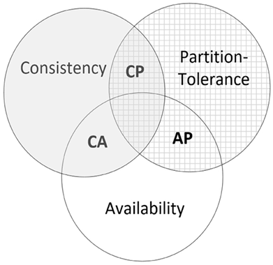
Figure 13.1: Visualizing the choices in distributed systems: the CAP theorem

Distributed data storage is increasingly becoming an essential component of modern IT infrastructure. Designing distributed data storage should be carefully considered, based on the characteristics of the data and the requirements of the problem we want to solve. When applied to distributed databases, the CAP theorem helps to guide the design and decision-making process by ensuring that developers and architects understand the fundamental trade-offs and limitations involved in creating distributed database systems. Balancing these three characteristics is crucial to achieve the desired performance, reliability, and scalability of the distributed database system. When applied to distributed databases, the CAP theorem helps to guide the design and decision-making process by ensuring that developers and architects understand the fundamental trade-offs. Balancing these three characteristics is crucial in order to achieve the desired performance, reliability, and scalability of the distributed database system. In the context of the CAP theorem, we can assume that there are three types of distributed storage systems:

• A CA system (implementing Consistency-Availability)
• An AP system (implementing Availability-Partition Tolerance)
• A CP system (implementing Consistency-Partition Tolerance)

Classifying data storage into CA, AP, and CP systems helps us to understand the various trade-offs involved when designing data storage systems.

Let’s look into them, one by one.

CA systems

Traditional single-node systems are CA systems. In non-distributed systems, partition tolerance is not a concern as there is no need to manage communication between multiple nodes. As a result, these systems can focus on maintaining both consistency and availability. In other words, they are CA systems.

A system can function without partition tolerance by storing and processing data on a single node or server. While this approach may not be suitable for handling large-scale data sets or high-velocity data streams, it can be effective for smaller data sizes or applications with less demanding performance requirements.

Traditional single-node databases, such as Oracle or MySQL, are prime examples of CA systems. These systems are well-suited for use cases where data volume and velocity are relatively low, and partition tolerance is not a critical factor. Examples include small to medium-sized businesses, academic projects, or applications with a limited number of users and data sources.

AP systems

AP systems are distributed storage systems designed to prioritize availability and partition tolerance, even at the expense of consistency. These highly responsive systems can sacrifice consistency, if necessary, to accommodate high-velocity data. In doing so, these distributed storage systems can handle user requests immediately, even if it results in temporarily serving slightly outdated or inconsistent data across different nodes.

When consistency is sacrificed in AP systems, users might occasionally may get slightly outdated information. In some cases, this temporary inconsistency is an acceptable trade-off, as the ability to quickly process user requests and maintain high availability is deemed more critical than strict data consistency.

Typical AP systems are used in real-time monitoring systems, such as sensor networks. High-velocity distributed databases, like Cassandra, are prime examples of AP systems.

An AP system is recommended for implementing distributed data storage in scenarios where high availability, responsiveness, and partition tolerance are essential.

For example, if Transport Canada wants to monitor traffic on one of the highways in Ottawa through a network of sensors installed at different locations on the highway, an AP system would be the preferred choice. In this context, prioritizing real-time data processing and availability is crucial to ensuring that traffic monitoring can function effectively, even in the presence of network partitions or temporary inconsistencies. This is why an AP system is often the recommended choice for such applications, despite the potential trade-off of sacrificing consistency.

CP systems

CP systems prioritize both consistency and partition tolerance, ensuring that distributed storage systems guarantee consistency before a read process retrieves a value. These systems are specifically designed to maintain data consistency and continue operating effectively even in the presence of network partitions.

The ideal data type for CP systems is data that requires strict consistency and accuracy, even if it means sacrificing the immediate availability of the system. Examples include financial transactions, inventory management, and critical business operations data. In these cases, ensuring that the data remains consistent and accurate across the distributed environment is of paramount importance.

A typical use case for CP systems is when we want to store document files in JSON format. Document datastores, such as MongoDB, are CP systems tuned for consistency in a distributed environment.

With an understanding of the different types of distributed storage systems, we can now move on to exploring data compression algorithms.

Decoding data compression algorithms

Data compression is an essential methodology used for data storage. It not only enhances storage efficiency and minimizes data transmission times, but it also has significant implications for cost savings and performance improvements, particularly in the realm of big data and cloud computing. This section presents the details data compression techniques, with a special focus on the lossless algorithms Huffman and LZ77, and their influence on modern compression schemes, such as Gzip, LZO, and Snappy.

Lossless compression techniques

Lossless compression revolves around eliminating redundancy in data to minimize storage needs while ensuring perfect reversibility. Huffman and LZ77 are two foundational algorithms that have strongly influenced the field.

Huffman coding focuses on variable-length coding, representing frequent characters with fewer bits, while LZ77, a dictionary-based algorithm, exploits repeated data sequences and represents them with shorter references. Let us look into them one by one.

Huffman coding: Implementing variable-length coding

Huffman coding, a form of entropy encoding, is used widely in lossless data compression. The key principle underlying Huffman coding is to assign shorter codes to more frequently occurring characters in a dataset, thereby reducing the overall data size.

The algorithm uses a specific type of binary tree known as a Huffman tree, where each leaf node corresponds to a data element. The frequency of occurrence of the element determines the placement in the tree: more frequent elements are placed closer to the root. This strategy ensures that the most common elements have the shortest codes.

A quick example

Imagine we have data containing letters A, B, and C with frequencies 5, 9, and 12 respectively. In Huffman coding:

• C, being the most frequent, might get a short code like 0.
• B, the next frequent, could get 10.
• A, the least frequent, might have 11.

To understand it fully, let us go through an example in Python.

Implementing Huffman coding in Python

We start by creating a node for each character, where the node contains the character and its frequency. These nodes are then added to a priority queue, with the least frequent elements having the highest priority. For this, we create a Node class to represent each character in the Huffman tree. Each Node object contains the character, its frequency, and pointers to its left and right children. The __lt__ method is defined to compare two Node objects based on their frequencies.

import functools
@functools.total_ordering
class Node:
    def __init__(self, char, freq):
        self.char = char
        self.freq = freq
        self.left = None
        self.right = None
    def __lt__(self, other):
        return self.freq < other.freq
    def __eq__(self, other):
        return self.freq == other.freq

Next, we build the Huffman tree. The construction of a Huffman tree involves a series of insertions and deletions in a priority queue, typically implemented as a binary heap. To build the Huffman tree, we create a min-heap of Node objects. A min-heap is a specialized tree-based structure that satisfies a simple but important condition: the parent node has a value less than or equal to its children. This property ensures that the smallest element is always at the root, making it efficient for priority operations. We repeatedly pop the two nodes with the lowest frequencies, merge them, and push the merged node back into the heap. This process continues until there is only one node left, which becomes the root of the Huffman tree. The tree can be built by build_tree function, which is defined as follows:

import heapq
def build_tree(frequencies):
    heap = [Node(char, freq) for char, freq in frequencies.items()]
    heapq.heapify(heap)
    while len(heap) > 1:
        node1 = heapq.heappop(heap)
        node2 = heapq.heappop(heap)
        merged = Node(None, node1.freq + node2.freq)
        merged.left = node1
        merged.right = node2
        heapq.heappush(heap, merged)
    return heap[0]  # the root node

Once the Huffman tree is constructed, we can generate the Huffman codes by traversing the tree. Starting from the root, we append a 0 for every left branch we follow and a 1 for every right branch. When we reach a leaf node, the sequence of 0s and 1s accumulated along the path from the root forms the Huffman code for the character at that leaf node. This functionality is achieved by creating generate_codes function as follows.

def generate_codes(node, code='', codes=None):
    if codes is None:
        codes = {}
    if node is None:
        return {}
    if node.char is not None:
        codes[node.char] = code
        return codes
    generate_codes(node.left, code + '0', codes)
    generate_codes(node.right, code + '1', codes)
    return codes

Now let us use the Huffman tree. Let us first define data that we will use for Huffman’s encoding.

data = {
    'L': 0.45,
    'M': 0.13,
    'N': 0.12,
    'X': 0.16,
    'Y': 0.09,
    'Z': 0.05
}

Then, we print out the Huffman codes for each character.

# Build the Huffman tree and generate the Huffman codes
root = build_tree(data)
codes = generate_codes(root)
# Print the root of the Huffman tree
print(f'Root of the Huffman tree: {root}')
# Print out the Huffman codes
for char, code in codes.items():
    print(f'{char}: {code}')

Root of the Huffman tree: <__main__.Node object at 0x7a537d66d240>
L: 0
M: 101
N: 100
X: 111
Y: 1101
Z: 1100

Now, we can infer the following:

• Fixed length code: The fixed-length code for this table is 3. This is because, with six characters, a fixed-length binary representation would need a maximum of three bits (2³ = 8 possible combinations, which can cover our 6 characters).
• Variable length code: The variable-length code for this table is

  45(1) + .13(3) + .12(3) + .16(3) + .09(4) + .05(4) = 2.24.

The following diagram shows the Huffman tree created from the preceding example:

Figure 13.2: The Huffman tree: visualizing the vompression process

Note that Huffman encoding is about converting data into a Huffman tree that enables compression. Decoding or decompression brings the data back to the original format.

Having looked at Huffman’s encoding, let us now explore another lossless compression technique based on dictionary-based compression.

Next, let us discuss dictionary-based compression.

Understanding dictionary-based compression LZ77

LZ77 belongs to a family of compression algorithms known as dictionary coders. Rather than maintaining a static dictionary of code words, as in Huffman coding, LZ77 dynamically builds a dictionary of substrings seen in the input data. This dictionary isn’t stored separately but is implicitly referred to as a sliding window over the already-encoded input, facilitating an elegant and efficient method of representing repeating sequences.

The LZ77 algorithm operates on the principle of replacing repeated occurrences of data with references to a single copy. It maintains a “sliding window” of recently processed data. When it encounters a substring that has occurred before, it doesn’t store the actual substring; instead, it stores a pair of values – the distance to the start of the repeated substring in the sliding window, and the length of the repeated substring.

Understanding with an example

Imagine a scenario where you’re reading the string:

data_string = "ABABCABABD"

Now, as you process this string left to right, when you encounter the substring "CABAB", you’ll notice that "ABAB" has appeared before, right after the initial "AB". LZ77 takes advantage of such repetitions.

Instead of writing "ABAB" again, LZ77 would suggest: “Hey, look back two characters and copy the next two characters!” In technical terms, this is a reference back of two characters with a length of two characters.

So, compressing our data_string using LZ77, it might look something like:

ABABC<2,2>D

Here, <2,2> is the LZ77 notation, indicating “go back by two characters and copy the next two.”

Comparison with Huffman

To appreciate the power and differences between LZ77 and Huffman, it’s helpful to use the same data. Let’s stick with our data_string = "ABABCABABD".

While LZ77 identifies repeated sequences in data and references them, Huffman encoding is more about representing frequent characters with shorter codes.

For instance, if you were to compress our data_string using Huffman, you might see certain characters, say 'A' and 'B', that are more frequent, represented with shorter binary codes than the less frequent 'C' and 'D'.

This comparison showcases that while Huffman is all about frequency-based representation, LZ77 is about spotting and referencing patterns. Depending on the data type and structure, one might be more efficient than the other.

Advanced lossless compression formats

The principles laid out by Huffman and LZ77 have given rise to advanced compression formats. We will look into three advanced formats in this chapter.

1. LZO
2. Snappy
3. gzip

Let us look into them one by one.

LZO compression: Prioritizing speed

LZO is a lossless data compression algorithm that emphasizes rapid compression and decompression. It replaces repeated occurrences of data with references to a single copy. After this initial pass of LZ77 compression, the data is then passed through a Huffman coding stage.

While its compression ratio might not be the highest, its processing speed is significantly faster than many other algorithms. This makes LZO an excellent choice for situations where quick data access is a priority, such as real-time data processing and streaming applications.

Snappy compression: Striking a balance

Snappy is another fast compression and decompression library originally developed by Google. The primary focus of Snappy is to achieve high speeds and reasonable compression, but not necessarily the maximum compression.

Snappy’s compression method is based on LZ77 but with a focus on speed and without an additional entropy encoding step like Huffman coding. Instead, Snappy utilizes a much simpler encoding algorithm that ensures speedy compressions and decompressions. The algorithm uses a copy-based strategy where it searches for repeated sequences in the data and then encodes them as a length and a reference to the previous location.

It should be noted that due to this tradeoff for speed, Snappy does not compress data as efficiently as algorithms that use Huffman coding or other forms of entropy encoding. However, in use-cases where speed is more critical than the compression ratio, Snappy can be a very effective choice.

GZIP compression: Maximizing storage efficiency

GZIP is a file format and a software application used for file compression and decompression. The GZIP data format uses a combination of the LZ77 algorithm and Huffman coding.

Practical example: Data management in AWS: A focus on CAP theorem and compression algorithms

Let us consider an example of a global e-commerce platform that runs on multiple cloud servers across the world. This platform handles thousands of transactions every second, and the data generated from these transactions needs to be stored and processed efficiently. We’ll see how the CAP theorem and compression algorithms can guide the design of the platform’s data management system.

1. Applying the CAP theorem

The CAP theorem states that a distributed data store cannot simultaneously provide more than two out of the following three guarantees: consistency, availability, and partition tolerance.

In our e-commerce platform scenario, availability and partition tolerance might be prioritized. High availability ensures that the system can continue processing transactions even if a few servers fail. Partition tolerance means the system can still function even if network failures cause some of the servers to be isolated.

While this means the system may not always provide strong consistency (every read receives the most recent write), it could use eventual consistency (updates propagate through the system and eventually all replicas show the same value) to ensure a good user experience. In practice, slight inconsistencies might be acceptable, for example, when it takes a few seconds for a user’s shopping cart to update across all devices.

In the AWS ecosystem, we have a variety of data storage services that can be chosen based on the needs defined by the CAP theorem. For our e-commerce platform, we would prefer availability and partition tolerance over consistency. Amazon DynamoDB, a key-value NoSQL database, would be an excellent fit. It offers built-in support for multi-region replication and automatic sharding, ensuring high availability and partition tolerance.

For consistency, DynamoDB offers “eventual consistency” and “strong consistency” options. In our case, we would opt for eventual consistency to prioritize availability and performance.

2. Using compression algorithms

The platform would generate vast amounts of data, including transaction details, user behavior logs, and product information. Storing and transferring this data could be costly and time-consuming.

Here, compression algorithms like gzip, Snappy, or LZO can help. For instance, the platform might use gzip to compress transaction logs that are archived for long-term storage. Given that gzip can typically compress text files to about 30% of their original size, this could reduce storage costs significantly.

On the other hand, for real-time analytics on user behavior data, the platform might use Snappy or LZO. While these algorithms may not compress data as much as gzip, they are faster and would allow the analytics system to process data more quickly.

AWS provides various ways to implement compression depending on the type and use of data. For compressing transaction logs for long-term storage, we could use Amazon S3 (Simple Storage Service) coupled with gzip compression. S3 supports automatic gzip compression for files being uploaded, which can significantly reduce storage costs. For real-time analytics on user behavior data, we could use Amazon Kinesis Data Streams with Snappy or LZO compression. Kinesis can capture, process, and store data streams for real-time analytics, and supports compression to handle high-volume data.

3. Quantifying the benefits

The benefits can be quantified similarly as described earlier.

Let’s take a practical example to demonstrate potential cost savings. Imagine our platform produces 1 TB of transaction logs daily. By leveraging gzip compression with S3, we can potentially shrink the storage requirement to roughly 300 GB. As of August 2023, S3 charges around $0.023 for every GB up to the initial 50 TB monthly. Doing the math, this equates to a saving of about $485 each month, or a significant $5,820 annually, just from the log storage. It’s worth noting that the cited AWS pricing is illustrative and specific to August 2023; be sure to check current rates as they might vary.

Using Snappy or LZO with Kinesis for real-time analytics could improve data processing speed. This could lead to more timely and personalized user recommendations, potentially increasing sales. The financial gain could be calculated based on the increase in conversion rate attributed to improved recommendation speed.

Lastly, by using DynamoDB and adhering to the CAP theorem, we ensure a smooth shopping experience for our users even in the event of network partitions or individual server failures. The value of this choice could be reflected in the platform’s user retention rate and overall customer satisfaction.

Summary

In this chapter, we examined the design of data-centric algorithms, concentrating on three key components: data storage, data governance and data compression. We investigated the various issues related to data governance. We analyzed how the distinct attributes of data influence the architectural decisions for data storage. We investigated different data compression algorithms, each providing specific advantages in terms of efficiency and performance. In the next chapter, we will look at cryptographic algorithms. We will learn how we can use the power of these algorithms to secure exchanged and stored messages.

Learn more on Discord

To join the Discord community for this book – where you can share feedback, ask questions to the author, and learn about new releases – follow the QR code below:

https://packt.link/WHLel