6 Some Number Theoretic Algorithms
6.1 Number Theoretic Algorithms for Public Key Cryptography
Number theory plays a prominent role in many areas of cryptography. In the simplest case, to develop a cryptosystem for an N letter alphabet, we consider the letters as integers modulo N. As described in Chapter 5, the integers modulo N form a ring called the modular ring ![]() N and encryption is done using algebraic operations on this ring. The totality of operations within the various modular rings is called modular arithmetic. The encryption algorithms then apply number theoretic functions and use modular arithmetic on these integers. Hence encryption maps on k-length message units are functions
N and encryption is done using algebraic operations on this ring. The totality of operations within the various modular rings is called modular arithmetic. The encryption algorithms then apply number theoretic functions and use modular arithmetic on these integers. Hence encryption maps on k-length message units are functions
In addition to providing a framework for the encrypted alphabets, number theoretic problems provide the security in the basic public key protocols. Recall that the security of a cryptographic protocol is usually based on the difficulty of solving some “hard” problems. The two most commonly used public key methods in cryptography are the Diffie-Hellman method and its variations and the RSA method and its variations. For the Diffie-Hellman method, the hard problem used for cryptography is the discrete log problem that we will discuss in depth in Section 6.5. The hard problem for the RSA method is the factorization problem, that is the relative difficulty of factoring large integers.
In this chapter we discuss these hard number theoretic problems and several important number theoretic algorithms related to them. We then discuss primality testing, that is determining whether or not an integer is prime. The relative difficulty of finding large primes versus factoring large integers provides the security in RSA and related cryptographic methods.
6.2 Quadratic Residues and Square Roots
If a є ![]() then we write ā for the residue class for a modulo n. Sometimes, especially in calculations, it is convenient to write just a as an element of
then we write ā for the residue class for a modulo n. Sometimes, especially in calculations, it is convenient to write just a as an element of ![]() n without any misunderstanding.
n without any misunderstanding.
Definition 6.2.1. If (a, m) = 1 and and x2 ≡ a (mod m) has a solution then a is called a quadratic residue modulo m. If x2 ≡ a (mod m) has no solution then a is a quadratic non-residue.
Further if x2 ≡ a (mod m) then x is a square root of a modulo m.
The basic idea in using quadratic residues in cryptography stems from the following. If n isa prime, then we can decide effectively if a is a quadratic residue modulo n or not. However if n = pq, the product of two distinct odd primes p and q, then in general there is no known probabilistic algorithm to decide if a is a quadratic residue modulo n unless p and q are known.
The following result sets up a probabilistic method for determining modular square roots by counting the number of quadratic residues and quadratic nonresidues modulo a prime.
Theorem 6.2.2. Let p ≥ 3 bean odd prime.
(1) The set {1, 2,…, p − 1} contains exactly ![]() quadratic residues and hence exactly
quadratic residues and hence exactly ![]() quadratic non-residues.
quadratic non-residues.
(2) If a є ![]() and (a, p) = 1 then a has 0 or 2 square roots modulo p, that is the equation x2 ≡ a (mod p) has 0 or 2 solutions modulo p
and (a, p) = 1 then a has 0 or 2 square roots modulo p, that is the equation x2 ≡ a (mod p) has 0 or 2 solutions modulo p
(3) If p is an odd prime and (a, p) = 1 then a is a quadratic residue modulo p if and only if a![]() ≡ 1 (mod p). If a is a quadratic non-residue then a
≡ 1 (mod p). If a is a quadratic non-residue then a![]() ≡ −1 (mod p).
≡ −1 (mod p).
(4) If a, b є ![]() with (a, p) = (b, p) = 1 then ab is a quadratic residue modulo p if both a and b are quadratic residues modulo p or if both a and b are quadratic non-residues modulo p.
with (a, p) = (b, p) = 1 then ab is a quadratic residue modulo p if both a and b are quadratic residues modulo p or if both a and b are quadratic non-residues modulo p.
Proof. (2) Consider the polynomial p(x) = x2 − ā є ![]() p [x]. If x0 is one solution of p(x) = 0 then −x0 is another. Since a quadratic polynomial over a field can have at most 2 zeros there are the only square roots of a. On the other hand if there is no solution the polynomial is irreducible and there are no square roots. (For more details see [CFR1].)
p [x]. If x0 is one solution of p(x) = 0 then −x0 is another. Since a quadratic polynomial over a field can have at most 2 zeros there are the only square roots of a. On the other hand if there is no solution the polynomial is irreducible and there are no square roots. (For more details see [CFR1].)
(1) Now x2 = (-x)2 (modp). Hence
in ![]() and 12, 22,…, (
and 12, 22,…, (![]() )2 are quadratic residues modulo p.
)2 are quadratic residues modulo p.
(3) Suppose (a,p) = We do the computations in the field ![]() p. Since a ≠ 0 then from Fermat’s Theorem ap-1 = - in
p. Since a ≠ 0 then from Fermat’s Theorem ap-1 = - in ![]() p. This implies that
p. This implies that
in ![]() p. Since
p. Since ![]() p is a field it has no zero divisors and this implies that either a
p is a field it has no zero divisors and this implies that either a![]() = 1 or a
= 1 or a ![]() = -1. Hence either a
= -1. Hence either a![]() ≡ 1(mod p)or a
≡ 1(mod p)or a![]() ≡ -1. We show that in the former case and only in the former case is a a quadratic residue.
≡ -1. We show that in the former case and only in the former case is a a quadratic residue.
Suppose that x2 = a has a solution say x0 in Zp. Then
It follows further that if a ![]() = -1 there can be no solution.
= -1 there can be no solution.
Conversely suppose a ![]() =1. Since the multiplicative group of Zp is cyclic (see the last section) it follows that there is a g e Zp which generates this cyclic group and t t(p-1) a = gL for some t. Hence g
=1. Since the multiplicative group of Zp is cyclic (see the last section) it follows that there is a g e Zp which generates this cyclic group and t t(p-1) a = gL for some t. Hence g![]() = 1. However the order of the multiplicative group of
= 1. However the order of the multiplicative group of ![]() p is p - 1 and therefore this implies that
p is p - 1 and therefore this implies that
Therefore t must be even t = 2k. Hence a = g2k = (gk)2 and there is a solution to x2 = a.
(4) This is a direct consequence of (3). □
We now introduce the Legendre symbol and use this to show how we can effectively decide, for (a, p) = 1 and p an odd prime, whether or not a is a quadratic residue. The restriction to odd primes is obvious because a = 1 (mod 2) for each odd integer a.
Definition 6.2.3. If p is an odd prime and (a,p) = 1 then the Legendre symbol ![]() is defined by
is defined by
(1) ![]() = 1 if a is a quadratic residue modulo p;
= 1 if a is a quadratic residue modulo p;
(2) ![]() = -1if a is a quadratic non-residue modulo p.
= -1if a is a quadratic non-residue modulo p.
Therefore the value of the Legendre symbol distinguishes quadratic residues from quadratic non-residues. The next lemma establishes the basic properties of ![]() .
.
Theorem 6.2.4. Ifp is an odd prime and (a, p) = (b, p) = 1 then
(1) ![]()
(2) ![]()
(3) ![]() = a
= a![]() (mod p)
(mod p)
(4) ![]()
(5) If a = p1p2 … pk is a prime factorization of a then
(6) ![]()
(7) ![]()
Proof. Parts (1) and (2) are immediate from the definition of the Legendre symbol.
Part (3) is a direct consequence of Lemma 2.6.1.
To see part (4) notice that (ab)![]() = a
= a![]() b
b![]() and use part (3). □
and use part (3). □
From part (4) of this last lemma we see that to compute ![]() we can use the prime factorization of a and then restrict to
we can use the prime factorization of a and then restrict to ![]() where q is a prime distinct from p. The quadratic reciprocity law which is presented next will allow us to compute this for odd primes and then use the result for (2). We present examples after the theorem on how to do this. There are many proofs of the quadratic reciprocity law. For more information we refer to [FR]. We now give the theorem.
where q is a prime distinct from p. The quadratic reciprocity law which is presented next will allow us to compute this for odd primes and then use the result for (2). We present examples after the theorem on how to do this. There are many proofs of the quadratic reciprocity law. For more information we refer to [FR]. We now give the theorem.
Theorem 6.2.5 (Law of Quadratic Reciprocity). If p,q are distinct odd primes then
Alternatively ifp, q are distinct odd primes then
(1) If at least one ofp, q is congruent to 1 modulo 4 then
x2 = q (mod p) and x2 = p (mod q)
are either both solvable or both unsolvable.
(2) If both p and q are congruent to 3 modulo 4 then one of
x2 = q (mod p) and x2 = p (mod q)
is solvable and the other is unsolvable.
For a proof of the quadratic reciprocity law and more details we refer to [FR].
Example 6.2.6. Letp = 1993 and q = 65 537 = 216 + 1. We show thatp is a quadratic non-residue modulo q.

Since the value of the Legendre symbol is -1 it follows that p is a quadratic nonresidue modulo q.
Example 6.2.7. Let p = 7 and a = 870. We show that a is a quadratic residue modulo p.
Since the value of the Legendre symbol is 1 if follows that a is a quadratic residue modulo p.
6.3 Modular Square Roots
We now describe a probabilistic algorithm to calculate square roots modulo an odd prime p. By a probabilistic algorithm, we mean an algorithm that will return either that an inputted integer a with (a, p) = 1 does not have a square root modulo p, or that a has a given degree of probability of having a square root.
Suppose first that p = 3 (mod 4). Then ![]() then
then
Since b -![]() = ±1 it follows that the whole expression equals ñb. Therefore
= ±1 it follows that the whole expression equals ñb. Therefore
is a square root of a and ±ap are the only square roots of a. Therefore in the case p = 3 (mod 4) we get the square roots of a modulo p by simple exponentiation.
Theorem 6.3.1. Let p be an odd prime and a e {1,…,p - 1} a quadratic residue modulo p. Then the following algorithm produces with arbitrary probability > 1 - (|)k a square root of a modulo p.
(1) Ifp = 3 (mod 4) then give a ~ modulo p and stop.
(2) Ifp = 1 (mod 4) write p - 1 = 2st with s > 2 and t odd.
(a) Choose a random u eZ* and compute u 2 . Repeat this as long asu 2 = -1 up to a maximum ofk times. Now calculate v = tf. t+1
(b) Determine y = a 2
(c) 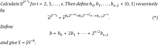
Proof. First we show that in part (c) we get a square root modulo p for a.
For i = s we get
and hence
We now show that we can realize the equation (*).
a is a quadratic residue modulo p so that a![]() = a2 t = 1 (modp). Then
= a2 t = 1 (modp). Then
On the other side
If a2 = 1 (modp) then choose b0 = 0 and if a2 ‘ = -1 (modp) then choose b0 = 1.
From this we get
Now we may construct b1, b2,…, bs-2 step by step. Recall that if we construct bj for j e {1,…, s - 2} then i = j +2 and
We now consider the situation n = pq with p, q two distinct primes.
Theorem 6.3.2. Letp, q > 2 be two distinct primes. Let a e Zwith (a, p) = (a, q) = 1. Then a is a quadratic residue modulo pq if and only if a is a quadratic residue modulo both p and q.
Proof. Suppose that x2 = a (modpq). Then directly x2 = a (modp)andx2 = a (mod q).
Conversely, suppose then x2 = a (mod p)andy2 = a (mod q). Then by the Chinese Remainder Theorem (see Chapter 5) there exists an integer z with z = x (mod p) and z = y (mod q). Then z2 = a (modp) andz2 = a (mod q) and hence also z2 = a (modpq). □
Theorem 6.3.3. Let n = pq with p, q two distinct odd primes. Let a be an integer with (a, p) = (b, p) = 1. Then the congruence x2 = a (mod n) has either 0 or 4 solutions modulo n.
If the prime factorization n = pq is known and if a is a quadratic residue modulo n then there exists a probabilistic algorithm to efficiently calculate the four solutions of x2 = a (mod n).
Proof. If the number a is a quadratic non-residue modulo n then the congruence x2 = a (mod n) has no solutions modulo n.
Now let a be a quadratic residue modulo n. We apply the Chinese Remainder Theorem to obtain a bijection
Then b eZ* and c eZ* are quadratic residues modulo p or modulo q respectively.
Hence there exist y eZ* and z eZ* with b = y2 and c = z2.
The residue classes
are pairwise distinct and satisfy
Hence
for i = 1, 2,3,4.
For the second part of the theorem we apply Theorem 6.3.1 to determine y and z. We can then apply the Chinese Remainder Theorem to calculate x1, x2, x3, x4. □
If n = pq, with p, q distinct large odd primes, then there is no known general probabilistic algorithm which can be applied to check efficiently if an integer a is a quadratic residue modulo n or not, unless the prime factors p and q are known.
We should mention the case where p | a or q | a. Here consider n = pq with p, q two distinct odd primes and suppose that a eZ.
(1) If we have p | a and (a, q) = 1, or if we have q| a and (a, p) = 1, then the congruence x2 = a (mod n) has either 0 or 2 solutions modulo n.
(2) If p | a and q | a then the congruence x2 = a (mod n) has only the solution 0 modulo n.
(3) Let n = 2p with p > 3 and let a be an integer.
(a) If 2 | a and (a, p) = 1 then the congruence x2 = a (mod n) has either 0or 2 solutions modulo n.
(b) If (2, a) = 1 and p|a then the congruence x2 = a (mod n) has either 0 or 1 solution modulo n.
(c) If 2 | a and p | a then the congruence x2 = a (mod n) has only the solution 0 modulo n.
If p and q are known in (2) and (3) then the solutions can be calculated as in Theorem 6.3.2 by applying the Chinese Remainder Theorem.
6.4 Products of Two Primes
The two most commonly used methods in constructing public key cryptosystems are the RSA method and the Diffie-Hellman method. The Diffie-Hellman method depends for its security on the supposed difficulty of the discrete log problem, which we will discuss in Section 6.5. The RSA method depends on the difficulty of factoring large integers of the form n = pq, with p, q distinct odd large primes. Here we show that there are important connections between the square root problem and the factorization problem.
Theorem 6.4.1. Letp and q be two distinct primes and n = pq. If there exists a probabilistic algorithm to efficiently determine a square root b modulo n for every quadratic residue a modulo n then there exists a probabilistic algorithm to factorize n.
Proof. We randomly choose an integer x e {1,…,n-1}.Wemayassumethat(x, n) = 1, otherwise we may factorize n. Hence we may also assume that p, q are odd primes with (x, p) = (x, q) = 1. Let c = x2 (mod n). Determine a square root a for x modulo n. The integer a is modulo n one of the four square roots of c (see last section). We have
Here |a - x| e {0,1,…, n - 1} because a, x e {1,…, n - 1}. There are four possibilities
(1) p | (a - x), q | (a - x) (a - x, n) = n,
(2) p | (a + x), q | (a + x) (a - x, n) = 1,
(3) p | (a - x), q | (a + x) (a - x, n) = p,
(4) p | (a + x), q | (a - x) (a - x, n) = q.
Since each of these four cases occurs with equal probability we get that d = (a - x, n) is a proper divisor of n with probability 1. Hence after k repetitions we may factorize n with probability 1 - (2)k in its prime factors. □
The preceding theorem, together with Theorem 6.5, show that the problem of factorizing n = pq and to determine square roots modulo n are probabilistically algorithmically equivalent.
We may extend the previous result as follows.
Theorem 6.4.2. Let n be a composite positive integer. Let x, y e Zwithx2 = y2 (mod n) and x not congruent to ±y modulo n. Then (x + y, n) and (x - y, n) are proper divisors ofn.
Proof. From x2 = y2 (mod n)wegetthatx2-y2 = 0(modn) and hence (x-y)(x + y) = kn for some integer k. Note that both x and y are not congruent to 0 modulo n and k = 0 because x is not congruent to y or -y modulo n.
Hence n is a divisor of (x + y)(x - y) but neither a divisor of x + y nor x - y, again because x is not congruent to ±y modulo n. Therefore (x - y, n) and (x + y, n) are proper divisors of n. □
Corollary 6.4.3. Let n = pq with p, q two distinct primes. Let x, y eZ with x2 = y2 (mod n) and x not congruent to ±y modulo n. Then |(x + y, n)| and |(x - y, n)| are the prime factors ofn.
Example 6.4.4.
(a) Let n = 7429,x = 227,y = 210. Then x2 - y2 = n and x - y = 17,x + y = 437. Therefore (x - y, n) = 17 is a proper divisor of n.
(b) Let n = 253,x = 17,y = 6. Then 172 = 62 (mod 253) andx - y =11, x + y = 23. Therefore (11, 253) = 11, (23,253) = 23 and 253 = (23)(11).
Note that if n = pq is the product of two distinct primes and we can find integers x, y with x2 = y2 (mod n) then we can factorize n. The problem of course is to find such x and y. There is a quite efficient probabilistic algorithm called the quadratic sieve method to find such x and y values.
The method works as follows. Let m = [ Vn] where [a] denotes the greatest integer function, that is the greatest integer less than or equal to a.
Then consider the polynomial
f(t) = (t + m)2 - n
and evaluate f (a) for a eZ. We then try to find the prime factorization
If we find a1,…,ar such that f(a … f(ar) = y2 (mod n) for some integer y, then we can define
x = (a1 + m) … (ar + m) (mod n)
and test if x is not congruent to y modulo n and x is not congruent to -y modulo n.
For more details see [LL1], [LL2] and [KKi].
Example 6.4.5 (This is an example from [Buc]). Let n = 7429 so that m = 86 and f(t) = (t + 86)2 - 7429.
We have f (1) = 872 - 7429 = 140 = 22-5-7andf(2) = 882-7429 = 315 = 32 · 5-7. It follows that
(87 · 88)2 = (2 · 3 · 5 · 7)2 (mod n)
and we define x = (87)(88) = 227 (mod n)andy = (2)(3)(5)(7) = 210 (mod n). Now take x = 227 and y =210 and we have the two integers from the quadratic sieve.
A variation of the quadratic sieve method is the Fermat factorization method. Here let n = pq withp, q distinct odd primes. Then t = p+q and s = p-q are integers satisfying
Suppose that we want to factor n = pq. Start with t = [ Vn] + 1. Then we determine t2 - n.If t2 - n = s2 for some s, then from the above equation we determine p = t + s and q = t - s.
If t2 - n is not a square we replace t by t + 1 and repeat the process. We continue until we get a square.
This methods works quite efficiently if |p - q| is small. In this case t = is only slightly bigger than Vn. If |p - q| is very large, then many iterations are needed to get the desired result.
A variation of the Fermat factorization method works with a small positive integer k, the starting value t = [ Vkn] + 1 and the values t2 - kn. Here if t2 - kn = s2 is a square then check (t + s, n) and (t - s, n).
Another probabilistic algorithm to factorize a composite number n eN that uses congruences is based on the following idea.
Let n e N be a composite integer. Assume that the prime number p divides n and that we have two integers x, y with x not congruent to y modulo n and x = y (modp). Let d = (x - y, n).
From p | (x - y) and p | n we obtain that p | d and so d = 1. From n not being a divisor of x - y we get that d = n. Hence 1 < d < n and d is a proper divisor of n.
Now if n = pq, for two distinct primes, then we have the factorization. Therefore we want to find such x, y for n = pq with two distinct odd primes. This can be done probabilistically applying Pollard’s p -algorithm.
We take an integer x0 to start and a function f (x). A suitable function is f (x) = x2 + c with an integer c and c = 0, -2. Then we recursively define x;+1 = f(x;). Define y e {0,1,…, n - 1} with xt = yt (mod n) for i = 0,1,
If p is a prime divisor (which so far we do not know) then there are i = j with yi = yj (modp), that is d = (y; - y;-, n) > 1. If in addition yj = yj then d = n because y;, yj e {0,1,…, n - 1}. Hence we must determine the values (y; - yj, n) for i = j.
Example 6.4.6. Let n = 1517 and x0 = y0 = 70 withf(x) = x2 + 1.
Then y7 = 1358 and y14 = 825 and we get (1358 - 825,1517) = 41.
There are also factorization methods utilizing the Theorems of Fermat and Euler. The next theorem shows the connection between the Euler phi function $ (n) and the factorization of n = pq with p, q distinct odd primes.
Theorem 6.4.7. Let n = pq with p, q distinct odd primes. Then the pair (p, q) can be efficiently calculated if and only if$ (n) can be efficiently calculated.
Proof. We have $ (n) = (p - 1)(q - 1) = n - p - q +1. Hence p + q = n + 1 - $ (n) and pq = n. Therefore p and q are exactly the two solutions of the quadratic equation
The following is necessary for our next factorization method.
Lemma 6.4.8. Let n = pq with p, q distinct odd primes. Suppose that there exists an even integer m > 2 with am = 1 in Zn for all a eZjJ. Assume that there exists ab eZ*n m with b2 = 1. Then m
(1) For at least 50 % of the residue classes a in Zn we have a2 = 1. _ _E — —2_
(2) Suppose that there exists an a eZp with a2 =1 in Zp. Then b2 = 1 for exactly m
50 % of the residue classes b eZp and b2 = -1 for the other 50 %.
The analogous result holds for q.
Proof.
(a) Let {a1,…, as} be the different residue classes in Z*n with a2 = 1.
Then the residue classes aib are pairwise distinct and satisfy
(b) If a = 1 in Z* then a = 1 in Zp for an integer k. The proof now follows from
Theorem 6.2. □
Now we describe a probabilistic algorithm for the factorization of n = pq based on Fermat’s and Euler’s theorems.
Theorem 6.4.9 (Pollard’s p - 1 method). Let n = pq with p, q distinct odd primes. Suppose that we know an integer m > 1 witham = 1 for all a e Z*n. In particular we have such an m if we know $ (n). Then we can efficiently determine the prime factors p and q with the following probabilistic algorithm:
(1) Check for many, say 100, randomly chosen integers a e {1,…, n - 1} with (a, n) = 1 m if a2 = 1. If this is the case then replace mby’j. m
(2) Repeat (1) as often as one has an a with a2 = 1. m
(3) For a randomly chosen a e {1,…,n − 1} with (a,n) = 1 and a2 = 1, calculate m p1 = (n, a2 − 1) and check ifp1 > 1. If this is the case then n is factored. Define q1 = n and return the pair (p1, q1).
(4) Repeat (3) as long as there is a p1 with p1 > 1.
This is a probabilistic algorithm that finds the factorization n = pq in finitely many steps with a probability close to 1.
Proof. We first remark that m must be even. If m were odd we would have contradicting the fact that a” = 1 for all a e Z*. By Lemma 6.4.1 part (a) there are at least 50 % of the residue classes a e ZjJ with a2 = 1 if there exists one such a. If we check N times in step (1) whether a2 = 1or a2 = 1in Z* then we have a probability
Hence the loop (1)-(2) gives with high probability an even integer m such that there is an a e ZjJ with a2 = 1.
Now we have two cases.
Case 1: (p − 1) | f or(q − 1) | f.
Suppose without loss of generality that (p − 1) | m. Then (q − 1) cannot divide m m because otherwise $ (n) = (p − 1)(q − 1) is a divisor of m contradicting a2 = 1in Z. Recall form Euler’s Theorem that a$(n) = 1 for all a eZjJ.
Hence c2 = 1 (modp) for all c e {1,…, n − 1} with (c, n) = 1 and there exists b e m {1,2,…, n−1} with (b, n) = 1 and b2 not congruent to 1 modulo q. By Lemma 6.4.2 part (b) there is therefore a b e {1,…, n − 1} with (b, n) = 1 and b~ =−1 (mod q).m m We cannot have (n, b2 − 1) = 1 or q or n since p | (b2 − 1) and q does not divide m m b2 − 1. Hence (n, b2 − 1) = p and n is factorized.
Case 2: (p − 1) does not divide m and (q − 1) does not divide m.
Then for b e{1,…, n − 1} with (b, n) = 1 we have four possibilities:
(a) b2 = 1 (modp)andb2 = 1 (modq);
(b) b2 = −1 (modp)andb2 = 1 (modq);
(c) b2 = 1 (modp)andb2 = −1 (modq);
(d) b2 = −1 (modp) andb2 = −1 (modq). 1 m
Hence with probability 2 we have b e {1,…, n − 1} with (b, n) = 1 and b2 = −1 (modp) and b~ = 1 (mod q) or b~ = 1 (modp) and b~ = −1 (mod q) and m _ we may factorize n as in Case (1). Recall that there is an a e Z with a2 = 1 in m Zn and hence a2 = −1in Zp or in Z^ by the Chinese Remainder Theorem. Now apply Lemma 6.4.1(b). In cases (a) and (d) we move to another b and repeat the calculations. ?
Corollary 6.4.10. Letn = pqwithp, q distinct odd primes. Then the following conditions are equivalent.
(1) If we know an integer e with (e, $ (n)) = 1 then we can efficiently find an integer d with ed = 1 (mod $ (n)).
(2) We can efficiently find the prime factors p and q of n.
Proof. Suppose that we assume (1), so we suppose that we know such a d. Then ed −1 is divisible by $ (n) = (p − 1)(q − 1) which is even. We then get aed-1 = 1 (mod n) for all integers a e {1,…,n − 1} with (a, n) = 1. This can be seen as follows.
There exists an integer r with ed = 1 + r(p − 1)(q − 1). Then and aed = a (mod n) by Fermat’s theorem and the Chinese remainder theorem. With n = ed − 1, which is even, we can calculate p and q with the probabilistic algorithm from the theorem. Hence we get (2).
Now suppose that we have (2) so that we know p and q.
Then $ (n) = (p − 1)(q − 1) and we can find an integer d with de = 1 (mod $ (n)) using the Euclidean algorithm. □
6.5 Discrete Logarithms and the Discrete Log Problem
Diffie-Hellman in 1976 developed the original public key cryptographic protocol using the discrete log problem. In this section we introduce this and also discuss two algorithms for attempted solutions of the problem. The basic idea is that in modular arithmetic it is easy to raise an element to a power but difficult to determine, given an element, if it is a power of another element. We define the problem in general.
Definition 6.5.1. If G is a finite group, such as the cyclic multiplicative group of Zp where p is a prime, and h = gk for some k, then a discrete logarithm or discrete log of h to the base g is any integer t with h = gt .We denote this by
In the Diffie-Hellman method, that we will discuss in Chapter 7, this is usually applied to the cyclic group Zp where p is a prime.
Example 6.5.2. If G = Z19 then 6 = log2(7) since 26 = 64 = 7 (mod 19).
The discrete log does not have to be unique as the next example shows.
Example 6.5.3. Let G = Z8. Then 2 = log3(1) since 32 = 1 (mod8). But also 4 = log3(1) since 34 = 1 (mod 8) and 3 and 4 are incongruent modulo 8.
Notice that if G = (g) is of order n and h = g with 1 < i < n then the discrete log of h is uniquely defined for the generator g, that is i is unique modulo n for g.
The discrete logarithm problem denoted also by DLP is then the following. Let G = (g) and h e G. Find x eZ such that h = gx.
The smallest non-negative x with this property is often called the discrete logarithm of h relative to the generator g.
Other than an exhaustive search there is no known algorithm to solve the discrete log problem. This makes it ideal then as a method to construct a one-way function. In the next two subsections we look at algorithms to attempt to find a solution.
6.5.1 Shank’s Baby Step Giant Step Algorithm (BSGS)
In this section we describe an algorithm, due to Shanks, to find a discrete log. This is called the baby step giant step algorithm which is abbreviated BSGS. Let G = (b) be a finite cyclic group and suppose that a e G. We will try to find algorithmically an integer x such that a = bx and hence x = logb a. We need an upper bound S eN for the order of G, that is | G| < S. Define
Then n2 > S and in particular x = logb a < n2. Thenx = qn + r with r e {0,1,…, n − 1} and q e {0,1,…, n} by the division algorithm.
We get a = bx = bqn+r so that ab-r = bqn. From this last equation we must find r and q to obtain the discrete logarithm x = qn + r. There are n possibilities for r and n +1 possibilities for q. Hence we have to make two list of group elements. The first is the baby step list given by
Now we compare both lists. A common element ab r = bqn in both lists gives the integers q, r and hence the discrete logarithm
There must be a common element because |G| < n2.
Example 6.5.4 (see [Buc]). Let G = Zp with p = 2017. The integer 5 is a primitive element in G that is Zp = (5). Suppose that we want to find x = log5(3). We can take n = 45 because 452 > 2016 = |G|.
We write down the baby step list r = 0,1,…, 44 and the giant step list for q = 0,1,…, 45 and find a common element for r =40 and q = 22. Hence
For practical implementation of the BSGS one can first calculate the giant step list because it is independent of the integer a and can be used several times. Then we calculate the baby step list and compare each value step by step to the giant step list. We need < 2n group operations and we must store n group elements. Therefore we get the following result describing the complexity of the BSGS algorithm (see Chapter 3).
Theorem 6.5.5. The complexity of the baby-step giant-step algorithm in a cyclic group G is o(VHgI).
It follows that if |G| > 2160 the BSGS algorithm is not very helpful due to the size of the necessary storage space. The problem of storage space is handled in the next algorithm we discuss, the Pollard p-method.
6.5.2 Pollard’sp-Algorithm
The second method we describe for finding discrete logarithms is called the Pollard p -algorithm. This method will handle some of the storage space problems of the BSGS algorithms. We first need the following.
Lemma 6.5.6. Let a, c eZ and n eN. Then the congruence ax = c (mod n) with (a, n) = d is solvable if and only ifdc. In this case there are exactly d solutions modulo n that are given by
where x0 is any solution of the reduced equation
For a proof of this we refer to the book [FR].
We can now give the Pollard p-algorithm for the discrete log problem. If G = (b) is a finite cyclic group and a e G then this algorithm consists of three steps.
Step (1): Divide G into three pairwise disjoint subsets G1, G2, G3 with 1 £ G2 and each of about the same size.
Step (2): Determine two integers s, t with as = bt in the following manner.
Produce a sequence inductively with x0 = 1 and
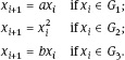
Then x1 e {a, b}, x2 e {a2, ab, b2} and so on. Altogether we get that x{ = aaibfoi for some au e Nu{0}.
Since G is finite there are indices i, j with i < j and x{ = x;-. We then have Setting produces the desired integers.
Step (3): Now determine the discrete log x = logb(a) as follows. Let s, t be as found in step (2). Then
bt = as = bsx since a = bx and so sx = t (mod n).
Hence x is a solution of the congruence
sx = t (mod n). (**)
Suppose that d = (s, n). By Lemma 6.5.2.1 the set of integer solutions to this congruence is
where x is the constructed solution.
Without loss of generality suppose that v is the smallest positive solution to (**) which we can find using the Euclidean algorithm. Since we may assume that the discrete logarithm is smaller than n we may assume that
Determine all values b d, k = 0,1,…,d − 1 and compare the results with a. This produces x = logb(a).
Example 6.5.7 (see [Buc]). As before let G = Zp with p = 2017. The integer 5 is a primitive element so that Zp = (5). We want to find x = log^(3). Take
G1 = {1,…, 672}, G2 = {673,…, 1344}, G3 = {1345,…, 2016}.
If we start with x0 = 1023 we get 5 =3 .Togetx we have to solve the congruence 128x = 800 (mod 2016). Doing this we get v = 22 and x = 22 + (16)(63). Recall that (128, 2016) = 32 and 63 = ^fj6.
The complexity of the Pollard p -algorithm in the finite cyclic group G is the same as that of the BSGS algorithm, namely O(VfG|). However this method is more storage efficient because we must only save one of the sets G1, G2, G3.
The two algorithms to solve the DLP can also be used to determine the order of an element in a finite abelian group.
Theorem 6.5.8. Let G be a finite abelian group and a e G. Suppose that B e N is a bound for the order of a, that is |a| < B (we could take B = | G| + 1). Then the following algorithm determines |a|.
Step (1): Letfo = min{k eN| k2 > B}. Thenfi2 > B. Determine a, a2, a3,…, afo .Define a1 = afo.
Step (2): Compute a1 for a = 1,…,fo and check if a1 e {a, a2,…,afo}. As soon as this is the case go to Step (3).
Step(3): If a1 = ar witha ,y e {1,…,fo} then factorize afo − y and find the smallest positive divisor S with as =1. The value S gives the order a of a.
Proof. Let n = |a| = oG(a) be the order of the element a in the group G. Write n = a1fo + y1 with a1, y1 e {0,…,fo − 1} by the division algorithm. This is possible since n < B < p2. Then
with a = a1 + 1 e { 1 ,…,fo} and y = -^ because a1 = cP .Inparticular y e { 1 ,…,fo}. Hence in (2) we must have a match a1 = ar. □
Finally we show how to reduce the DLP in a finite cyclic group to the DLP for cyclic groups of prime order.
Theorem 6.5.9. Let G1 = (g1) and G2 = (g2) be finite cyclic groups with (|G1|, |G2|) = 1. Let G = G1 x G2 = (g) withg = (g1,g2). Leta = (a1, a2) e G. Ifx = logg(a) then
Proof. Let x = logg(a) so that gx = a and hence (g^,g’2) = (a1, a2). Then gf = aj = gy with x = y (mod |G;|), 0 < y < |G;| for i = 1,2. Hence x = logg(a;) (mod |G;|) for i = 1,2. i □
Corollary 6.5.10. Let G, G1, G2, g be as in the above theorem. If we know the discrete logarithms x{ = logg. (a;), i = 1,2 then we can determine x = logg(a).
Proof. Since (|G;|, |G2|) = 1 we can apply the Chinese Remainder Theorem and obtain the result. □
This provides the reduction of the DLP to cyclic groups of prime power orders.
Example 6.5.11 (see [KKi]). Let G = Zp with p = 73. A primitive element modulo 73 is 5 so that G = (5).
We have the decompositionp − 1 = 72 = 2332.
We want to determine x = log^(58).
We get G = G1 x G2 with
and
For a = 58 we get the decomposition a = 58 = (589,58s) = (51, 55). Now
using the BSGS algorithm.
Now we apply the Chinese remainder theorem for
x ≡ 3 (mod 8) x ≡ 7 (mod 9).
This gives the solution x = 43 (mod 72). Hence logj(58) = 43 and 543 = 58.
Finally we can reduce the DLP to cyclic groups of prime order.
Theorem 6.5.12. Let G = (g) be a cyclic group with |G| = pn with p a prime and n > 1.By taking the logarithm n times we can reduce the DLP for G to the DLP for groups oforder p.
Proof. If n = 1 there is nothing to prove. Suppose n > 2. For an induction suppose that the result holds for cyclic groups of order pn-1.
Let U = < gp >. Then U is a subgroup of G of order pn-1. The factor group G/U is a cyclic group of order p (see [CFR1]) with G/U = (gU). Let a e G. Determine y eN with a = (gU)y = gyU. Then ag-y e U = (gp). From the inductive hypothesis we may determine an integer x by taking the logarithm (n − 1) times such that ag-y = gpx. Hence a = gy+px.
We now describe the procedure. Let G = (g) be a finite cyclic group of order pn with p prime and n > 1. Let a e G and suppose we want to find the discrete log x = logg(a). We write
with x0,.. .,xn−1 e {0,1,…,p − 1}. We determine x0,.. .,xn−1 step by step from the equation
gx = gx0+x1p+-+xn−1p”-1 = a (*)
and get x = logg(a) this way.
Recall that gp = 1. We first determine x0.
Fromgx = awe getgp 1x = (gp 1)x° = ap”1 becausegp” = 1.
Now gpn 1 has order p and we determine
We then determine x1 from the equation
ag-*0 = gx1p+-+x,−1p”-1.
and we determine
*1 = loggp'−1 (ap g~p x°).
. v.n-2 n-2 v
g pn- (a
gp
Now continue in the analogous manner to determine x2,…, xn_1 if necessary. □
Example 6.5.13 (see [KKi]). Let G = (g) with |G| = 53. We realize G as a subgroup of index 2 in Z251.
We have Z251 = < 6 > and hence G = < 6 2 >= < 36 >. We determine x = log^(4). Write x = x0 + 5x1 + 52x2 with x0, x1, x2 e {0,1,2,3,4} and determine x0, x1, x2 in
steps. From 36 = 4weget that (36 )x° = 4 =1, that is x0 = 0.
5x +52x ° 25 5
From 36 1 2 =4 • 36 = 4weget(36 )x1 = 4 =2°, that is
x1 = log-25 (20) = 2.
Therefore we obtain
Then (36 )x2 = 149 and x2 = log—25(149) = 4. Altogether
In general, this algorithm determines n discrete logarithms x0, x1,…, xn_1 in the cyclic group (gp ) of order p, and finally the desired discrete logarithm x in (g) of order pn.
Summarizing all these reductions we have the following.
Theorem 6.5.14. Let Gbe a finite cyclic group of order p^ p^2 •••p^ with this being the prime decomposition. Then the DLP for G can be reduced to the DLP in cyclic groups of orders pv…, pk.
Note that if |G| has only small prime factors then the DLP for G is relatively easy to solve. For example suppose that |G| = 2104344549747 and is cyclic. Then the DLP is solved in cyclic groups of orders 2,3,5,7, respectively.
6.5.3 The Index Calculus Method (ICM) for ZjJ
Given a prime number p > 3, the index calculus method or ICM is a method to determine probabilistically the discrete logarithm k of b where b = g and g is a primitive root modulo p. The method is done with the following steps.
Step (1): Choose a good bound B with B > 2. For a positive integer B the factor base is given by
F(B) = {g|g is a prime number with q < B}.
Let v = |F(B)| andp1 < p2 < ••• < pv be primes with p1 = 2 so that F(B) = {pv…,pv}.
Step (2): Choose randomly and equally distributed an integer
a € {1,…,p − 1}
and factorga modulop, that is, factor the integer c € {1,…,p − 1} withga = c (mod p).
We say that ga modulo p is B-smooth if each prime factor of ga modulo p is in F(B). If this is the case, then save a, ga modulo p and the prime factorization of ga modulo p.
Repeat this step as long as there are at least v piecewise different B-smooth values and each pi € F(B) occurs at least once.
Step (3): Let a1,…,av be the exponents of the pairwise different B-smooth values gai modulo p,…,gav modulo p found in Step 2. Then
with
From this we get the system of congruences
If all loggp), i = 1,…, v, occur, then solve the system for these loggp).
If this system is not solvable, then determine more B-smooth values as in Step 2 and continue as long as the system is solvable.
Step(4): Choose randomly and equally distributeds € {1,…,p − 1} as long as bgs modulo p is B-smooth. Then
Take the discrete logarithms, loggp), j = 1,…, v, as found in Step 2, and put them into the congruence
and solve this for k = logg(b).
This is a probabilistic algorithm which gives uniquely the discrete log, k = logg(b) modulo (p − 1) of b, for the generator g of Z*.
The first step in the ICM algorithm is to find an optimal bound B. Then, for the complexity of the ICM algorithm most significant is the complexity of a good factorization algorithm to factor the values ga modulo p which is in general subexponential in log p. Having this in mind and combining this with the described steps we get that the ICM algorithm is subexponential in log p. More details can be found in the book by S. S. Wagstaff Jr. [Wag].
6.6 Primality Testing
We now consider the question of determining whether a particular given positive integer n is prime or not prime. The methods used in solving this problem are called primality testing and consist of algorithms to determine whether or not an inputted positive integer is prime. Primality testing is extremely important due to its close ties to public key cryptography. We will be looking at public key methods carefully in the next chapter. Both the Diffie-Hellman method and the RSA method, the two main public key techniques, require the user to determine large primes. The security of these methods depends on the fact that it is easier to determine large primes than to factor large integers.
At first glance, the problem of determining if a positive integer n is prime, seems like an easy one. If n is not prime it must have a divisor m with 1 < m < n. Therefore test all integers 2,…, 2 to see if they divide n or not. If there is such a divisor then n is composite. If not, then n is prime.
Of course this can be improved on in several ways. First of all, if n = mk is a non-trivial factorization, that is 1 < m < n, 1 < k < n, then one of m or k must be
< Vn. Hence to check for primality we need only check divisibility of n by integers from 2 to Vn rather than from 2 to 2. Further if n has a divisor m with 1 < m < Vn, then n must have a prime divisor p with 1 < p < Vn. Therefore it is only necessary to check the primes < Vn. Therefore knowing all the primes < Vn provides the necessary knowledge to test all the integers < n for primality. We summarize all these comments to give an elementary general algorithm for primality testing.
General Algorithm for Primality Testing
Given n > 0, test all primes p with p < Vn. The integer n is prime if and only if none of these primes divides n.
Example 6.6.1. Test whether the integer 83 is prime.
Now 9 < V83 < 10 so we must test all the primes less than 9. Hence we must test 2,3,5, 7. None of these divides 83 and therefore 83 is prime.
This general algorithm is simple and always works. However it becomes computationally infeasible for large integers. Therefore other methods become necessary to determine primality. Most of these methods rely on a number theoretic property, such as Fermat’s Theorem, which is true for all primes but may not be true for all compos- ites. Recall that Fermat’s Theorem says that ap 1 = 1 (modp) for any prime p and for any a with 1 < a < p. We will return to these shortly.
6.6.1 Sieving Methods
Another set of techniques for determining primes are called sieving methods. In ordinary language a sieve is a device to separate, or sift, finer particles from coarser particles. This idea has been applied to number theory via numerical sieving methods. A sieve in number theory is a method or procedure to find numbers with desired properties (for example primes) by sifting through all the positive integers up to a certain bound, successively eliminating invalid candidates until only numbers with the particular attributes desired are left. Sieving methods are quite effective for obtaining lists of primes (and numbers with other characteristics) up to a reasonably small limit.
Relative to generating lists of primes, sieving methods originated with the Sieve of Eratosthenes. This is a straightforward method to obtain all the primes less than or equal to a fixed bound x. It is ascribed (as the name suggests) to Eratosthenes (276−194 B. C.) who was the chief librarian of the great ancient library in Alexandria. Besides the sieve method he was an influential scientist and scholar in the ancient world, developing a chronology of ancient history (up to that point) and helping to obtain an accurate measure (within the measurement errors of his time) of the dimensions of the Earth.
The method of the Sieve of Eratosthenes is direct and works as follows. Given x > 0 list all the positive integers less than or equal to x. Starting with 2, which is prime, cross out all multiples of 2 on the list. The next number on the list, not crossed out, which is 3, is prime. Now cross out all the multiples of 3 not already eliminated. The next number left uneliminated, 5, is prime. Continue in this manner. As explained for the primality test described in the previous section the elimination must only be done for numbers < VX. Upon completion of this process, any number not crossed out must be a prime.
Below we exhibit the Sieve of Eratosthenes for numbers < 100. In beginning each round of elimination we must only consider numbers < V100 = 10.

After completing the sieving operation we obtain the list
{2,3, 5, 7,11,13,17,19, 23, 29,31, 37,41,43, 47, 53, 59, 61, 67, 71, 73,
79,83, 89,97}
which comprises all the primes less than or equal to 100.
6.6.2 Fermat’s Primality Testing
A primality test is an algorithm which inputs a positive integer n and outputs whether it is prime or not. These tests can be subclassified as either deterministic primality tests or probabilistic primality tests. In a deterministic test an integer n is inputted and the output is, yes the integer is prime, or, no the integer is not prime. Hence both the direct method of trial division and the Sieve of Eratosthenes are deterministic tests.
A non-deterministic primality test takes an inputted integer n and returns either no it is not prime or it may be a prime. A probabilistic primality test is a non- deterministic test that returns either the inputted integer is not a prime or is probably a prime to some given degree of accuracy. There are various tests which can give this accuracy to as high a probability as desired. Numbers that pass a probabilistic primality test are called probable primes. For use in cryptography, knowing if an integer is prime to a high probability, is often just as good as knowing if it is definitely prime. For this reason probable primes with a high degree of probability are called industrial grade primes, a term originally coined by M. Cohen.
The majority of probabilistic tests are based on either Fermat’s Theorem or some variation of it. If n is an integer and suppose that a is relatively prime to n with a”-1 not congruent to 1 modulo n. Then n cannot be prime. This is usually called the Fermat Probable Prime Test. Basically given n we find an a with (a, n) = 1 and compute a”-1 modulo n. If this value is not 1 modulo n, then n is not prime. If it is congruent to 1 modulo n, then n may be prime. In the latter case, by trying different values for a we can assign a probability value. We will make this precise. The basic Fermat Probable Prime Test is the following.
The Fermat Probable Prime Test
Suppose n is an inputted integer. Find an a with (a, n) = 1. Compute a”-1 modulo n. If this value is not 1 modulo n then n is not prime. If this value is 1 modulo n then n may be prime.
Example 6.6.2. Test whether 11387 is prime.
This integer is relatively small so even by trial division determining whether it is prime is easy. We use the Fermat method just to illustrate the technique.
Start with a = 2 and we test 211386 modulo 11387. The basic idea is to use repeated squarings to reduce the congruence. All the equivalences are modulo 11387.

Continuing in this manner we eventually get
From Fermat’s theorem if n is prime we would have an-1 = 1 (mod n) and therefore an = a (mod n). Here 4321 is not congruent to 2 modulo 11 387. Therefore 11 387 is not prime.
For this integer using trial division it is easy to obtain the factorization
11387 = (59)(193).
However even with an integer this size a calculator at least is necessary.
There are several methods to make Fermat testing deterministic. In 1891 Lucas gave the following extension of Fermat’s Theorem.
Theorem 6.6.3 (Lucas). Let n > 1. If for every prime factor p ofn − 1 there exists an integer a such that
(1) an-1 = 1 (mod n) and
n−1
(2) a p is not congruent to 1 modulo n.
Then n is prime.
Proof. Suppose n satisfies the conditions of the theorem. To show that n is prime we will show that $ (n) = n − 1 where $ is the Euler phi function. Since in general $ (n) < n − 1, to show equality we will show that under the above conditions n − 1 divides $ (n). Suppose not. Then there exists a primep such that pr divides n − 1, but pr does not divide $ (n) for some exponent r > 1. For this prime p, there exists an integer a satisfying the conditions of the theorem. Let m be the order of a modulo n. Then m divides n − 1 since the order of an element divides any power which equals 1 (see Chapter 5). However by the second condition in the theorem and for the same reason, m does not divide k Therefore pr divides m which divides $ (n) contradicting our assumption. Hence n − 1 = $ (n) and therefore n is prime. □
The following result is related.
Theorem 6.6.4. Suppose that a, k, n, q €N with n − 1 = qk and q > k. Suppose further that
(1) q is prime;
(2) an-1 = 1 (mod n);
Then n is prime.
Proof. Suppose that n is not prime. Then there exists a prime divisorp of n withp < Vn Let d be the order of a in Z*. From (2) we get that an-1 = 1 (modp), that is d | (n − 1).
From (3) we get that d does not divide k for otherwise p | (ak − 1) and p | n.
From (1) we not get that q | d. Suppose that q does not divide d. Then q | m f n − 1 = dm − qk. Hence k = dm and d | k which gives a contradiction. Therefore q | d.
Altogether we have
since d | (p − 1). But q > V” from q > k which gives a contradiction. It follows that n is a prime number. □
Example 6.6.5. Show that 2922 259 is a prime number.
We get the factorization 2922 259 − 1 = 1721 • 1698. We find that 1721 is prime and apply the theorem with k = 1698. Computing we find that
and hence applying the theorem the number is prime.
Although these tests are deterministic, they are, in most cases, no more computationally feasible than trial division or sieving, since the tests depend on the factorization of n −1. In general, factorization is even more difficult than solely testing for primality. Therefore, even here, further methods are necessary. We note that the idea in the Lucas Test has been quite effective in developing methods for testing Fermat and Mersenne numbers for primality.
Primality testing is essentially a computational problem. Therefore a primality test raises questions about the accompanying algorithm’s computational speed and computational complexity. For these types of number theoretic algorithms the computational complexity is measured in terms of functions of the input length, which here is roughly the number of digits of the inputted integer. The Sieve of Eratosthenes requires, for an inputted integer n, roughly the same order n of operations. If n has log10 n digits Then the Sieve requires 0(10log10 n) operations to prove primality. We say that this algorithm is of exponential time in terms of the input length. The big open question was whether there existed a deterministic algorithm which was of polynomial time in the input length. This means, that for this algorithm there is a positive integer d such that the number of operations in the algorithm to prove primality is O((log n)d). Earlier, Miller and Rabin had shown that the Miller-Rabin Test, which we will describe later in this section, can be made deterministic. Further it is of polynomial time if one accepts as true the extended Riemann hypothesis (see [FR]). However, prior to 2003 it was an open question whether there was a deterministic algorithm for primality which could be shown to be of polynomial time without using any unproved conjectures.
In 2003, M. Agrawal and two of his students, N. Kayal and N. Saxena, developed an algorithm, now called the AKS Algorithm, which was deterministic and could be proved to be of polynomial time. The result was even more spectacular since it was accomplished with relatively elementary methods. The basic algorithm depends on two rather straightforward extensions of Fermat’s Theorem. This result has of course generated a great deal of attention and much has already been written about it. We refer the reader to the articles [Bor] and [Ber] for a more complete discussion of the algorithm and its development and to [FR] for a more complete discussion of the algorithm as well as its proof.
To handle the computational problems probabilistic tests were introduced. To repeat what we defined earlier, a non-deterministic primality test takes an inputted integer n and returns either no it is not prime or it may be a prime. A probabilistic primality test is a non-deterministic test that returns either the inputted integer is not a prime or is probably a prime to some given degree of accuracy.
6.6.3 Pseudoprimes and Probabilistic Primality Testing
In a probabilistic primality test a number that can possibly be a prime is called a probable prime. Here we look at some probable primes for the Fermat probabilistic test.
Definition 6.6.6. Let n be a composite integer. If b > 1 with (n, b) = 1 Then n is a pseudoprime to the base b if bn-1 = 1 (mod n).
If n is a pseudoprime to the base b then it passes the Fermat Test and hence is a probable prime.
Example 6.6.7. 25 is a pseudoprime to the base 7. To see this notice that
This implies that 74 = 1 (mod 25) and hence 724 = 16 = 1 (mod 25).
Notice that 25 is not a pseuodprime modulo 2 or 3.
Theorem 6.6.8. For each base b > 1 there exists infinitely many pseudoprimes to the base b.
Proof. Suppose b > 1. We show that if p is any odd prime not dividing b2 − 1 then the integer n = pcf is a pseudoprime to the base b. Note that for this n we have
so that n is composite.
Given b, from Fermat’s Theorem we have bp = b (modp) and hence b2p = b2 (modp). Now n − 1 = bb2−1 and since p does not divide b2 − 1 by assumption it follows that p divides n − 1.