Chapter 5
Probability Theory
Package(s): prob, scatterplot3d, ConvergenceConcepts
5.1 Introduction
Probability is that arm of science which deals with the understanding of uncertainty from a mathematical perspective. The foundations of probability are about three centuries old and can be traced back to the works of Laplace, Bernoulli, et al. However, the formal acceptance of probability as a legitimate science stream is just a century old. Kolmogorov (1933) firmly laid the foundations of probability in a pure mathematical framework.
An experiment, deterministic as well as random, results in some kind of outcome. The collection of all possible outcomes is generally called the sample space or the universal space. An example of the universal space of a deterministic experiment is the distance traveled as a consequence of the application of some force is ![]() . On the other hand, for a random experiment of tossing a coin, the sample space consists of the set {Head, Tail}. The difference between these two types of experiments is the result of the final outcome. For a stationary object, if the application of a force results in an acceleration of
. On the other hand, for a random experiment of tossing a coin, the sample space consists of the set {Head, Tail}. The difference between these two types of experiments is the result of the final outcome. For a stationary object, if the application of a force results in an acceleration of ![]() , the distance traveled after 60 seconds is known by the formula
, the distance traveled after 60 seconds is known by the formula ![]() . That is, given the acceleration and time, the distance is uniquely determined. For a random experiment of coin tossing, the outcome is sometimes a Head, and at the other times it is Tail.
. That is, given the acceleration and time, the distance is uniquely determined. For a random experiment of coin tossing, the outcome is sometimes a Head, and at the other times it is Tail.
In this chapter, we will mainly focus on the essential topics of probability which will be required during rest of the book. We begin with the essential elements of probability and discuss the interesting problems using mathematical thinking embedded with in R programs. Thus, we begin with the sets and elementary counting methods and compute probabilities using the software in Section 5.2. Combinatorial aspects with useful examples will be treated in Section 5.3. The subject of measure theory is rightly required and we then discuss the core concepts required for the developments unfolding in Section 5.4. Conditional probability, independence, and Bayes formula are dealt with in Sections 5.5 and 5.6. Random variables and their important properties are detailed in Section 5.7. Convergence of random variables and other important sequences of functions of random variables are discussed through Sections 5.9–5.12. We emphasize here that you may sometimes come across phrases such as “graphical proof ”, or “it follows from the diagram that …”. In most of these cases, the general statement holds true and admits an analytical proof, which actually means that it is the more mathematical proof that is admitting a cleaner visual display. The reader is cautioned here though that such visual displays do not necessarily imply that the mathematical proof is valid and hence we must resist the temptation to generalize statements based on the displays. The spirit adopted in this chapter in particular is to emphasize that probability concepts can be integrated well with a software and that programming may sometimes be viewed as the e-version of problem solving skills.
5.2 Sample Space, Set Algebra, and Elementary Probability
The sample space, denoted by ![]() , is the collection of all possible outcomes associated with a specific experiment or phenomenon. A single coin tossing experiment results in either a head or a tail. The difference between the opening and closing prices of a company's share may be a negative number, zero, or a positive number. A (anti-)virus scan on your computer returns a non-negative integer, whereas a file may either be completely recovered or deleted on a corrupted disk of a file storage system such as hard-drive, pen-drive, etc. It is indeed possible for us to consider experiments with finite possible outcomes in R, and we will begin with a few familiar random experiments and the associated set algebra.
, is the collection of all possible outcomes associated with a specific experiment or phenomenon. A single coin tossing experiment results in either a head or a tail. The difference between the opening and closing prices of a company's share may be a negative number, zero, or a positive number. A (anti-)virus scan on your computer returns a non-negative integer, whereas a file may either be completely recovered or deleted on a corrupted disk of a file storage system such as hard-drive, pen-drive, etc. It is indeed possible for us to consider experiments with finite possible outcomes in R, and we will begin with a few familiar random experiments and the associated set algebra.
It is important to note that the sample space is uniquely determined, though in some cases we may not know it completely. For example, if the sequence {Head, Tail, Head, Head} is observed, the sample space is uniquely determined under binomial and negative binomial probability models. However, it may not be known whether the governing model is binomial or negative binomial. Prof G. Jay Kerns developed the prob package, which has many useful functions, including set operators, sample spaces, etc. We will deploy a few of them now.
Mahmoud (2009) is a recent introduction to the importance of urn models in probability. Johnson and Kotz (1977) is a classic account of urn problems. These discrete experiments are of profound interest and are still an active area of research and applications.
Note that the sample space may be treated as a super set. It has to be exhaustive, covering all possible outcomes. Loosely speaking we may say that any subset of the sample space is an event. Thus, we next consider some set operations, which in the language of probability are events.
Let ![]() be two subsets of the sample space
be two subsets of the sample space ![]() . The union, intersection, and complement operations for sets is defined as follows:
. The union, intersection, and complement operations for sets is defined as follows:
- The union of two sets
 and
and  is defined as:

- The intersection of two sets
 and
and  is defined as:

- The complement of a set
 is defined as:
- The set difference, or relative complement, of set
 and
and  is defined by

Software, and hence R, despite their strengths, will be used to illustrate the above using simple examples.
We will now consider a few introductory problems for computation of probabilities of events, which are also sometimes called elementary events. If an experiment has finite possible outcomes and each of the outcomes is as likely as the other, the natural and intuitive way of defining the probability for an event is as follows:
where ![]() denotes the number of elements in the set. The number of elements in a set is also called the cardinality of the set.
denotes the number of elements in the set. The number of elements in a set is also called the cardinality of the set.
It is also the case that even for elementary events, all the outcomes are not necessarily equally likely. The next example is a point in case.
5.3 Counting Methods
The events of interest may unfold in a number of different ways. We need mechanisms to find in how many different ways an event can occur. As an example, if we throw two die and count the sum of the numbers that appear on the two faces, the sum of 8 can occur in six different ways, viz., (6,2), (2,6), (5,3), (3,5), (4,4), (4,4). In this section, we will discuss some results which will be useful for a large class of problems and theorems.
The seasoned probabilist Kai Lai Chung has registered the importance of the role of permutations and combinations in a probability course. Over a period of years, he has obtained different answers for the number of ways a man can dress differently from a combination of three shirts and two ties. The answers vary from ![]() and
and ![]() to
to ![]() and
and ![]() . See page 46, Chung and AitSahlia (2003).
. See page 46, Chung and AitSahlia (2003).
A natural extension of the above experiment is shown by the next result.
At the outset, the fundamental theorem of counting may appear very simple. Its strength will be used to derive the total number of ways a task can be done in the next subsection.
5.3.1 Sampling: The Diverse Ways
Sampling from a population can be carried out in many different ways. Suppose that we have ![]() balls in an urn, and each ball carries a unique label along with it. Without loss of generality, we can label the balls 1 to
balls in an urn, and each ball carries a unique label along with it. Without loss of generality, we can label the balls 1 to ![]() . In this case we say that the balls are ordered. If the label of the balls carry no meaning, or are not available, that is, indistinguishable, we are dealing with sampling problems with unordered units.
. In this case we say that the balls are ordered. If the label of the balls carry no meaning, or are not available, that is, indistinguishable, we are dealing with sampling problems with unordered units.
5.3.1.1 Sampling with Replacement and with Ordering
Consider the situation where we draw ![]() units sequentially from
units sequentially from ![]() units. Before each draw, the balls in the urn are shaken well so that any ordered ball has the same chance of being selected. At each stage after the draw, the label of the drawn unit is noted and the order of labeled units is duly recorded before placing it back in the urn. Thus, if
units. Before each draw, the balls in the urn are shaken well so that any ordered ball has the same chance of being selected. At each stage after the draw, the label of the drawn unit is noted and the order of labeled units is duly recorded before placing it back in the urn. Thus, if ![]() denotes the label of the unit drawn on the
denotes the label of the unit drawn on the ![]() occasion, we have an ordered
occasion, we have an ordered ![]() - tuple
- tuple ![]() , with
, with ![]() taking a value between
taking a value between ![]() ,
, ![]() . The fundamental counting theorem then gives the answer of doing this task in
. The fundamental counting theorem then gives the answer of doing this task in
distinct ways.
5.3.1.2 Sampling without Replacement and with Ordering
Suppose that the experiment remains the same as above, with a variation being that the drawn ball is not put back in the urn. That is, at the first draw we have ![]() units to choose from. At the second draw, we have
units to choose from. At the second draw, we have ![]() units to choose from, at the third draw
units to choose from, at the third draw ![]() units, and so on. Thus, at the
units, and so on. Thus, at the ![]() draw, we have
draw, we have ![]() units for drawing the unit. Thus, sampling with replacement from ordered units can be performed in
units for drawing the unit. Thus, sampling with replacement from ordered units can be performed in ![]() distinct ways. Since we cannot draw more than
distinct ways. Since we cannot draw more than ![]() units among
units among ![]() , we have the constraint of
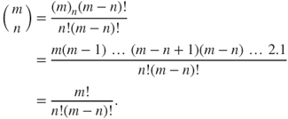
, we have the constraint of ![]() . We have again applied the fundamental theorem of counting. Let us introduce a notation here of continued product:
. We have again applied the fundamental theorem of counting. Let us introduce a notation here of continued product: ![]() to denote
to denote ![]() . That is
. That is
In popular terms, this is the permutation of ![]() units sampled from a pool of
units sampled from a pool of ![]() units. An interesting case is the permutation of obtaining all the
units. An interesting case is the permutation of obtaining all the ![]() units. This experiment is about drawing all the units without replacement from the urn and is given by
units. This experiment is about drawing all the units without replacement from the urn and is given by
To see the behavior of the number of ways we can possibly draw, let us look at the permutation of drawing 1 to 12 units.
> sapply(1:12,factorial)
[1]  1 2 6 24 120 720 5040  40320 362880
[10] 3628800  39916800 479001600
The sapply function ensures that the factorial function is applied on each integer 1 to12.
5.3.1.3 Sampling without Replacement and without Ordering
We now consider a sampling variation of the previous experiment. In this experiment we do not record the order of the occurrence of the sampling unit. Alternatively, we can think of this experiment as seeing the final result of sampling the desired number of ![]() units. We have seen that a sample of
units. We have seen that a sample of ![]() units can be obtained in
units can be obtained in ![]() different ways. Furthermore, the number of distinct ways of obtaining a sample of
different ways. Furthermore, the number of distinct ways of obtaining a sample of ![]() units from
units from ![]() is given by the continued product
is given by the continued product ![]() . Thus, the number of ways of obtaining an unordered sample of
. Thus, the number of ways of obtaining an unordered sample of ![]() units by sampling without replacement from
units by sampling without replacement from ![]() units is
units is ![]() . By multiplying the numerator and denominator by
. By multiplying the numerator and denominator by ![]() , we get the desired result
, we get the desired result
5.3.1.4 Sampling with Replacement and without Ordering
In this setup, we draw ![]() balls one after another, replacing the drawn ball in the urn before the next draw. During this process, we register the frequencies of the labels drawn with possible repetitions without storing the order of occurrence. Note that in this case
balls one after another, replacing the drawn ball in the urn before the next draw. During this process, we register the frequencies of the labels drawn with possible repetitions without storing the order of occurrence. Note that in this case ![]() may be less than
may be less than ![]() .
.
We summarize all the results in the table above.
5.3.2 The Binomial Coefficients and the Pascals Triangle
The Pascal's triangle is a simplistic and useful triangle for obtaining the binomial coefficients. To begin with, consider the following relationship:
This relationship says that to obtain ![]() , we can obtain it as the sum of ways of selecting
, we can obtain it as the sum of ways of selecting ![]() and
and ![]() objects from
objects from ![]() . Thus, we can move to higher levels using the quantities at one level below it. This leads to the famous Pascal's triangle. A short program is given below to obtain the triangle.
. Thus, we can move to higher levels using the quantities at one level below it. This leads to the famous Pascal's triangle. A short program is given below to obtain the triangle.
> pascal <- function(n){
+ if(n<=1) pasc=1
+ if(n==2) pasc=c(1,1)
+ if(n>2){
+ pasc <- c(1,1)
+ j <- 2
+ while(j<n){
+     j <- j+1
+     pasc=c(1,as.numeric(na.omit(filter(pasc,rep(1,2)))),1)
+ }
+ }
+ return(pasc)
+ }
> sapply(1:7, pascal)
[[1]]
[1] 1
[[2]]
[1] 1 1
[[3]]
[1] 1 2 1
[[4]]
[1] 1 3 3 1
[[5]]
[1] 1 4 6 4 1
[[6]]
[1]  1  5 10 10  5  1
[[7]]
[1]  1  6 15 20 15  6  1
With the basics of combinatorics with us, we are now equipped to develop R solutions for some interesting problems in probability.
5.3.3 Some Problems Based on Combinatorics
Feller (1968) has a very deep influence on almost all the Probabilists. Diaconis and Holmes (2002) considered some problems from Feller's Volume 1 in the Bayesian paradigm. Particularly, we consider two of those three problems here: (i) The Birthday Problem, and (ii) The Banach Match Box Problem. The problems selected here serve the point that probability on some occasions can be very counter-intuitive. A survey of some of these problems may also be found in Mosteller (1962).
The next R program gives us the birthday probabilities where we compute the probability of obtaining the same birthday if there are 2, 5, 10, 20, …, 50, people in a classroom.
> k <- c(2,5,10,20,30,40,50)
> probdiff <- c(); probat2same <- c()
> for(i in 1:length(k))  {
+   kk <- k[i]
+   probdiff[i] <- prod(365:(365-kk+1))/(365^{k}k)
+   probat2same[i] <- 1- prod(365:(365-kk+1))/(365^{k}k)
+                         }
> plot(k,probat2same,xlab="Number of Students in Classroom",
+      ylab="Birthday Probability",col="green","l")
> lines(k,probdiff,col="red","l")
> legend(10,1,"Birthdays are not same",box.lty=NULL)
> legend(30,.7,"Birthdays are same",,box.lty=NULL)
> title("A: The Birthday Problem")
The R numeric vectors probdiff and probat2same respectively compute ![]() and
and ![]() . The code
. The code prod(365:(365-kk + 1))/(365^kk)!birthday probability"?> gives ![]() , and by using it we easily obtain
, and by using it we easily obtain probat2same. The plot functions, lines, legend, and title are simple to follow.
Table 5.1 Diverse Sampling Techniques
| ordered = True | ordered = False | |
| replace = True | ||
| replace = False |
The birthday probabilities are summarized in Table 5.2. It can be seen from the table that we need to have just 50 people in a classroom to be almost sure of finding a pair of birthday mates. Part A of Figure 5.2 gives the visual display of the table probabilities. The meeting point of the complementary curves at 0.5 gives k=23 as claimed in Williams (2001).□
Table 5.2 Birthday Match Probabilities
| Size k | Probability of Different Birthdays | Probability of at least Two Same Birthdays |
| 2 | 0.9973 | 0.0027 |
| 5 | 0.9729 | 0.0271 |
| 10 | 0.8831 | 0.1169 |
| 20 | 0.5886 | 0.4114 |
| 30 | 0.2937 | 0.7063 |
| 40 | 0.1088 | 0.8912 |
| 50 | 0.0296 | 0.9704 |

Figure 5.2 Birthday Match and Banach Match Box Probabilities
We will now digress a little here and have a close look at the failure of the definition of probability discussed thus far. It seems to our intuition that if ![]() , the probability for any subset
, the probability for any subset ![]() must exist. That is, any subset
must exist. That is, any subset ![]() must have a well defined measure. Ross and Pekoz (2007) consider a very elegant example of a subset
must have a well defined measure. Ross and Pekoz (2007) consider a very elegant example of a subset ![]() for which the measure cannot be defined in any rational way. Suppose that we begin at the top of a unit circle and take a step of one unit radian in a counter-clockwise direction. If required, we may perform more than one loop. The task is then computation of the probability of returning to the point from which we started our journey. Suppose that it takes
for which the measure cannot be defined in any rational way. Suppose that we begin at the top of a unit circle and take a step of one unit radian in a counter-clockwise direction. If required, we may perform more than one loop. The task is then computation of the probability of returning to the point from which we started our journey. Suppose that it takes ![]() steps and
steps and ![]() loops to return to the top of the circle. This implies that
loops to return to the top of the circle. This implies that ![]() . As
. As ![]() is an irrational number, it cannot be expressed as the ratio of two integers
is an irrational number, it cannot be expressed as the ratio of two integers ![]() . Thus, the probability of returning to the start point cannot be measured.
. Thus, the probability of returning to the start point cannot be measured.
This and some other limitations of the definition of probability considered up to now are overcome using the Kolmogorov's definition of probability, which is based on Measure Theory. We will leave out the details of these important discussions!
5.4 Probability: A Definition
We will begin with a few definitions and lemmas.
5.4.1 The Prerequisites
Let us consider a class of sets of ![]() , say
, say ![]() . The sequence
. The sequence ![]() is said to be monotone increasing if
is said to be monotone increasing if ![]() for each
for each ![]() . The sequence is said to be monotone decreasing if
. The sequence is said to be monotone decreasing if ![]() for each
for each ![]() . We introduce two sequences infimum
. We introduce two sequences infimum ![]() and supremum
and supremum ![]() as below:
as below:
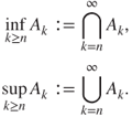
The symbol ![]() is used to convey that the quantity on the left-hand side is by definition equal to that on the right-hand side. It is easier to see that the
is used to convey that the quantity on the left-hand side is by definition equal to that on the right-hand side. It is easier to see that the ![]() sequence is monotone increasing sequence, whereas the
sequence is monotone increasing sequence, whereas the ![]() sequence is a monotone decreasing sequence. We further define sequences
sequence is a monotone decreasing sequence. We further define sequences ![]() and
and ![]() as follows:
as follows:

It is also common to refer to the couplet ![]() as a field. It may be easily proved that a field is also closed under finite union.
as a field. It may be easily proved that a field is also closed under finite union.
In plain words, the minimal field is the least collection of sets containing ![]() , which is a field.
, which is a field.
Fields need a generalization and especially in the case of countably infinite or continuous set ![]() .
.
The couplet ![]() is sometimes called the
is sometimes called the ![]() -field.
-field.
As earlier, we can define the minimal ![]() -field as an extension of the minimal field. There is an important class of
-field as an extension of the minimal field. There is an important class of ![]() -field, which will be defined now.
-field, which will be defined now.
It may be verified that the Borel ![]() -field consists of the intervals, for all
-field consists of the intervals, for all ![]() , of the following types:
, of the following types:
|
|
|
The definition of ![]() may be extended to
may be extended to ![]() and the reader may refer to Chung (2001). Starting with the sample space
and the reader may refer to Chung (2001). Starting with the sample space ![]() , a general class of sets
, a general class of sets ![]() has been defined. Next a formal definition of a measure is required.
has been defined. Next a formal definition of a measure is required.
Let us now look at two important types of measures.
We are now equipped with the necessary tools for a proper construction of a probability measure.
5.4.2 The Kolmogorov Definition
Here, the finiteness refers to the collection of sets in ![]() and additiveness refers to disjoint collection of events. Any set
and additiveness refers to disjoint collection of events. Any set ![]() is called an event or (more precisely) a measurable event. Next, we list some properties of the finitely additive probability measure:
is called an event or (more precisely) a measurable event. Next, we list some properties of the finitely additive probability measure:
 .
. .
.- If
 , then
  .
.  .
.- The General Additive Rule:
 , and hence
  .
. - For an arbitrary set
 and a collection of mutually exclusive and exhaustive sets
  :
:
We now extend the finitely additive probability measure to the countably infinite case.
5.5 Conditional Probability and Independence
An important difference measure theory and probability theory is in the notion of independence of events. The concept of independence is brought through conditional probability and its definition is first considered.
The next examples deal with the notion of conditional probability.
Conditional probabilities help in defining independence of events.
Some properties of the independence, if events ![]() and
and ![]() are independent, are listed as:
are independent, are listed as:
 and
and  are independent.
 and
and  are independent.
 and
and  are independent.
5.6 Bayes Formula
An excellent exposition of the the Bayes formula is provided in Chapter 4 of Bolstad (2007). Consider a partition of the sample space ![]() in a collection of
in a collection of ![]() events
events ![]() , also defined earlier in Section 5.4, from the probability space
, also defined earlier in Section 5.4, from the probability space ![]() . That is,
. That is, ![]() . Consider an arbitrary event
. Consider an arbitrary event ![]() . Then
. Then ![]() . Since
. Since ![]() 's form a partition of
's form a partition of ![]() , it can be visualized from the Venn diagram, Figure 5.4, that
, it can be visualized from the Venn diagram, Figure 5.4, that ![]() 's are also a disjoint set of events. Hence,
's are also a disjoint set of events. Hence,
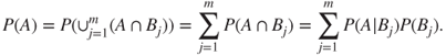
Figure 5.4 Venn Diagram to Understand Bayes Formula
The last step of the above expression is obtained by the multiple rule of probability. The beauty of Bayes formula is that we can obtain inverse probabilities, that is, the probability of the cause given the effect. This famous Bayes formula is given by:
5.7 Random Variables, Expectations, and Moments
5.7.1 The Definition
Sample events on their own are not always of interest, as we may only be interested in general events. For instance, if 100 coins are thrown, we may not be interested in the probabilities of the event itself, but we may question the number of heads in the range of 10 to 40, or > 80. Thus, we need to consider functions of the events which help to answer generic questions. This will lead us to the concept of random variable.
In plain words, it is required that for any Borel set ![]() , the inverse image
, the inverse image ![]() must belong to
must belong to ![]() :
:
A random variable will be simply abbreviated as RV. A commonly accepted convention is to denote the random variables by capital letters ![]() ,
, ![]() ,
, ![]() , etc., and the observed values by small letters
, etc., and the observed values by small letters ![]() ,
, ![]() ,
, ![]() , etc. respectively. Random variables are identified to be of three types: (i) simple random variable, (ii) elementary random variable, and (iii) extended random variable. A random variable
, etc. respectively. Random variables are identified to be of three types: (i) simple random variable, (ii) elementary random variable, and (iii) extended random variable. A random variable ![]() is said to be simple if there exists a finite partition of
is said to be simple if there exists a finite partition of ![]() in
in ![]() ,
, ![]() finite, implying
finite, implying ![]() , such that
, such that
where ![]() if
if ![]() and 0 otherwise. The random variable
and 0 otherwise. The random variable ![]() is said to be elementary if for a countably infinite partition of
is said to be elementary if for a countably infinite partition of ![]() in
in ![]()
Finally, the random variable ![]() is said to be an extended random variable if
is said to be an extended random variable if ![]() . An extended RV is often split into a positive part and a negative part defined by
. An extended RV is often split into a positive part and a negative part defined by
It can be easily seen that ![]() .
.
We next consider some important properties of random variables.
Properties of Random Variables
- Borel function
 of a random variable
  is also a random variable.
 - If
 is an RV, then
  is also a RV for
  .
. - Let
 and
and  be two RVs in a probability space
  . Then
  and
and  are also RVs.
 - Consider an independent sequence of RVs
 . Define, for all
  ,
,

Then
 ,
,  ,
,  , and
, and  are all RVs.
 - If
 converges as
  for every
  , then
  is also an RV.
An RV is better understood through important summaries such as mean and variance. We next define expectation of RV, which further helps in obtaining these summaries.
5.7.2 Expectation of Random Variables
As an introductory, the expectation of a discrete RV is defined by ![]() , and for a continuous RV, by
, and for a continuous RV, by ![]() . In light of the three types of RV discussed earlier, we need to now define the expectation of an RV for simple, elementary, and extended RVs defined in a probability space
. In light of the three types of RV discussed earlier, we need to now define the expectation of an RV for simple, elementary, and extended RVs defined in a probability space ![]() . For the moment, we will assume that the extended RVs are non-negative RVs.
. For the moment, we will assume that the extended RVs are non-negative RVs.
The expectations of simple RV and elementary RV as defined respectively in Equations 5.10 and 5.11 are given by
The expectation of a non-negative random variable is defined by

It may be noted that the limit can be ![]() too. The expectation of an arbitrary (extended) RV, as given in Equation 5.12, is defined by
too. The expectation of an arbitrary (extended) RV, as given in Equation 5.12, is defined by
provided that at least one of ![]() and
and ![]() is finite. If both
is finite. If both ![]() and
and ![]() are infinite, the expectation of the RV is not defined.
are infinite, the expectation of the RV is not defined.
Let us now consider some properties of expectations of RVs.
Properties of Expectation of Random Variables
- If
 and
and  are two partitions of a simple RV
  such that

then
- If
 is a non-negative and simple RV, then
  . This property continues to hold for non-negative RVs too.
 - If
 and
and  are two non-negative (simple or otherwise) RVs, and
  , then
  . This property is also known as the linearity of expectations.
The third counter-intuitive problem from Diaconis and Holmes (2002) will be discussed next.
Higher-order expectations are of interest for many RVs.
The forthcoming section will consider three important functions related to an RV.
5.8 Distribution Function, Characteristic Function, and Moment Generation Function
Let ![]() be an
be an ![]() -measurable random variable in the probability space
-measurable random variable in the probability space ![]() .
.
Properties of the cdf
- a. The cdf
 is a non-decreasing function, that is,
- b. The cdf
 is right-continuous:
- c.
 as we approach the null set.
 - d.
 as we approach
  .
. - e. The set of discontinuity points of
 is at most countable.
A related function is now defined.
We list below some properties of the mgf, and the reader can refer to Gut (2007) for details.
Properties of the mgf
- a. If the mgf
 is finite (in the above sense), the
  moment of
  is the
  derivative (w.r.t.
  ) of the mgf
  evaluated at
  .
. - b. Define
 ,
,  , where the mgf of
  is finite. Then
- c. A finite mgf determines the distribution of the RV uniquely.
The mgf does not exist for many important RVs, and thus we look at a function which will always exist.
The cf always exists for any random variable.
Properties of the cf
- a.
 ,
,  ,
,  .
. - b.
 is uniformly continuous on the real line.
 - c.
 .
.
The concepts of cdf, mgf, and cf will be illustrated in more detail in Sections 6.2–6.4.
5.9 Inequalities
The first inequality which comes to mind is the triangle inequality. It is claimed that this inequality has more than 200 different proofs! In probability theory, inequalities are useful when we do not have enough information about the distribution of the random variables. We will have practical scenarios where me may not know about the experiments any more than the fact that the random variables are independent, their mean, and probably standard deviation. We will now see the role of probabilistic inequalities.
5.9.1 The Markov Inequality
5.9.2 The Jensen's Inequality
The Jensen's inequality is a very useful technique, especially when we deal with the theory of the subject.
5.9.3 The Chebyshev Inequality
Consider a random variable ![]() with mean
with mean ![]() and variance
and variance ![]() . The Chebyshev's inequality states that
. The Chebyshev's inequality states that
This inequality has a very useful interpretation: “Not more than ![]() of the distribution's values can be more than
of the distribution's values can be more than ![]() standard deviations away from the mean.” Note that the inequality does not make any assumptions about the probability distribution of
standard deviations away from the mean.” Note that the inequality does not make any assumptions about the probability distribution of ![]() .
.
A one-tailed version of the Chebyshev's inequality is
The forthcoming section will deal with various convergence concepts of RVs.
5.10 Convergence of Random Variables
The concept of convergence is very strongly built in the ![]() argument. As Jiang (2010) emphasizes, the convergence concept embeds in itself the
argument. As Jiang (2010) emphasizes, the convergence concept embeds in itself the ![]() argument. Jiang refers to this tool as the A-B-C of large sample theory, and we will first discuss this in Example 1.1.
argument. Jiang refers to this tool as the A-B-C of large sample theory, and we will first discuss this in Example 1.1.
In the rest of this section, we attempt to gain an insight into using R programs and to establish the results analytically.
5.10.1 Convergence in Distributions
Consider a sequence of probability spaces ![]() , and let the random variable sequence
, and let the random variable sequence ![]() be such that for each
be such that for each ![]() ,
, ![]() is
is ![]() - measurable and
- measurable and ![]() . Furthermore, let
. Furthermore, let ![]() be the cumulative distribution function associated with
be the cumulative distribution function associated with ![]() . Also, let
. Also, let ![]() be another probability space and we consider an
be another probability space and we consider an ![]() -measurable random variable
-measurable random variable ![]() , whose
, whose ![]() associated cumulative probability distribution function is
associated cumulative probability distribution function is ![]() . Then we say that the sequence
. Then we say that the sequence ![]() converges in distribution to
converges in distribution to ![]() if as
if as ![]()
The standard notation for convergence in distribution is ![]() or
or ![]() . Sometimes the convergence in the distribution is also denoted by
. Sometimes the convergence in the distribution is also denoted by ![]() .
.
We next state an important result, see page 259 of Rohatgi and Saleh (2000).
The above theorem is now illustrated through an example.
5.10.2 Convergence in Probability
Consider a probability space ![]() and let
and let ![]() be a sequence of random variables defined in this space. We say that the sequence
be a sequence of random variables defined in this space. We say that the sequence ![]() converges in probability to a random variable
converges in probability to a random variable ![]() if for each
if for each ![]()

Symbolically, we denote this as ![]() .
.
Convergence in probability implies convergence in distribution. However, the converse is not true.
5.10.3 Convergence in  Mean
Mean
We begin with a probability space ![]() and let
and let ![]() be a sequence of random variables defined in it. We say that the sequence
be a sequence of random variables defined in it. We say that the sequence ![]() converges in
converges in ![]() mean to an RV
mean to an RV ![]() if
if ![]() and as
and as ![]()
5.10.4 Almost Sure Convergence
Let ![]() be a sequence of random variables on the probability space
be a sequence of random variables on the probability space ![]() . The sequence
. The sequence ![]() is said to converge almost surely to a RV
is said to converge almost surely to a RV ![]() if
if
The next result is very useful in establishing almost sure convergence. Almost sure convergence is denoted by ![]()
5.11 The Law of Large Numbers
The “large” in the Law of Large Numbers, abbreviated as LLN, is a pointer that the number of observations are very large. This clarification is issued in interest of the student community, as we felt that quite a few of them have confused the “large” with the magnitude of ![]() .
.
The LLN has two very important variants: (i) the Weak Law of Large Numbers, abbreviated as WLLN, and (ii) the Strong Law of Large Numbers, SLLN. The former is a convergence in probability criteria and the latter is almost sure convergence. Formal statements are given here. We discuss the concepts with a few analytical illustrations.For an understanding of these concepts through simulation, we refer the reader to Section 6 of Chapter 12.
5.11.1 The Weak Law of Large Numbers
Let ![]() be a sequence of random variables and define
be a sequence of random variables and define ![]() . The sequence
. The sequence ![]() is said to obey the weak law of large numbers, WLLN, with respect to a sequence of constants
is said to obey the weak law of large numbers, WLLN, with respect to a sequence of constants ![]() ,
, ![]() , if there exists a sequence of constants
, if there exists a sequence of constants ![]() which satisfies
which satisfies
The sequence ![]() is called centering sequence and the sequence
is called centering sequence and the sequence ![]() is called norming sequence. We state below a result which helps to determine whether the WLLN holds true for the sequence under consideration.
is called norming sequence. We state below a result which helps to determine whether the WLLN holds true for the sequence under consideration.
5.12 The Central Limit Theorem
5.12.1 The de Moivre-Laplace Central Limit Theorem
A complete de-mystification of the de Moivre-Laplace CLT appears in Ramasubramaniam (1997). Suppose that ![]() . Let
. Let ![]() . Define
. Define
We will begin with a statement of this result.
Typically, CLT is demonstrated using a simulation study. Though that approach is not wrong, we would like to make a few pointers here. In a simulation study we actually use the realized values of the RVs as in ![]() . However, the CLT is truly about the convergence of RVs as in
. However, the CLT is truly about the convergence of RVs as in ![]() . The principal point is that we cannot pretend that
. The principal point is that we cannot pretend that ![]() is the same as
is the same as ![]() . Thus, our illustration, at least in this section, will not resort to a simulation study.
. Thus, our illustration, at least in this section, will not resort to a simulation study.
We give an animated version of the convergence in the following program.
> n <- 10:1000
> p <- 0.4
> for(i in 1:length(n)){
+     plot(0:n[i],dbinom(0:n[i],p=0.4,n[i]),
+     "h",xaxt="n",yaxt="n",xlab="x",ylab="PDF")
+     title("The de Moivre's Laplace Central Limit Theorem")
+     curve(dnorm(x,mean=n[i]*0.4,sd=sqrt(n[i]*0.4*0.6)),
+     from=0,to=n[i],add=TRUE)
+ }
Change the values of ![]() for different levels and enjoy the convergence. Consider the general iid case next.
for different levels and enjoy the convergence. Consider the general iid case next.
5.12.2 CLT for iid Case
Let ![]() be iid random variables with finite first and second moments, that is,
be iid random variables with finite first and second moments, that is, ![]() . Define
. Define ![]() . Let
. Let ![]() and
and ![]() denote the mean and variance for
denote the mean and variance for ![]() . The general CLT for the iid case is stated below.
. The general CLT for the iid case is stated below.
Two equivalent forms of the CLT statement are that as ![]()
This statement appears very generic and we consider an illustration with varied distributions.
The more general case of a sequence of independent RVs is considered next.
5.12.3 The Lindeberg-Feller CLT
The previous theorem along with Equation 5.26 handles a sequence of iid RVs. An extension of this result for the more generic case of a sequence of independent RVs is then required. The Lindeberg-Feller theorem gives a set of necessary and sufficient conditions which help establish CLT for a sequence of independent RVs. A few notations are in order towards this end.
Let ![]() be a sequence of RVs, and let their respective probability spaces be defined by the sequence
be a sequence of RVs, and let their respective probability spaces be defined by the sequence ![]() . In the case of the iid sequence, we have
. In the case of the iid sequence, we have ![]() . Assume that
. Assume that ![]() , and
, and ![]() . Define
. Define ![]() ,
, ![]() , and
, and ![]() . It may be noted by the reader here that
. It may be noted by the reader here that ![]() does not correspond to the realized value of the sum
does not correspond to the realized value of the sum ![]() . The next theorem is the famous result sought in this section.
. The next theorem is the famous result sought in this section.
From a programming perspective, it is better to first consider the simpler case of a sequence of iid RVs for verifying the Feller condition 5.27 and also the Lindeberg condition 5.28. It will become more clear why the simpler case has been considered first.
A stronger, but more restrictive, condition can be imposed, which can be used for examining the CLT for a sequence of independent RVs.
5.12.4 The Liapounov CLT
The Liapounov's CLT is given in the next theorem.
Since the Liapounov's condition 5.29 requires a higher-order moment condition, it is more difficult in general to establish whether it holds for a given sequence of RVs. However, it is sometimes very useful for a sequence of discrete RVs.
5.13 Further Reading
A futile exercise is being undertaken now as we promise the reader a complete bibliography on the sources of probability! With the possibility, that is positive probabilities, of some abuse, we have further classified the sources into different subsections.
5.13.1 Intuitive, Elementary, and First Course Source
Chung and AitSahlia (2004) is an appealing beginner's starting point. Chung and AitSahlia (2004) is a fourth edition enhancement of Chung (1979), which has been an excellent introduction since its first print. A higher secondary school introduction to probability has been written by two eminent Russian probabilists Gnedenko and Khinchin (1964). Ash (1969), Chandra and Chatterjee (2001), Gnedenko (1978), Durrett (2009), and Ross (2010) are some of the competitive first course texts on probability theory.
As far as intuition is concerned, one of the unrivalled works in the literature ever is the two volumes of Feller (1968 and 1971). A testimony and tribute to this fact is that almost any decent work on probability theory will cite Feller.
5.13.2 The Classics and Second Course Source
Feller's (1968 and 1971) two volumes are intuitive, classic, advanced courses, and also almost everything else too. The measure theoretic approach was first detailed in Kolmogorov (1933). This short book served as a cornerstone for the way probability would be written from that point onward. It is generally agreed that Loéve (1955) has been the first comprehensive take on the measure theoretic approach to probability and the last edition of his work appeared in two volumes, Loeve (1977). Chung (2000) has been another famous probabilitist researcher who has also written some of the best probability books.
Ash and Doléans-Dade (2000), Shiryaev (1995), Chow and Teicher (1995), Athreya and Lahiri (2005), Durrett (2010), and Breiman (1962, 1992), among others, are some of the excellent measure theoretic approaches to probability. Parthasarathy (1978) and Billingsley (1995) have also stood the test of time and are still a favorite of many probability readers. In most of the books mentioned in this paragraph, the first editions have appeared a couple of decades earlier than their most recent editions that we have listed here.
Rosenthall (2006) and Kallenberg (2002) are two of the modern texts on measure theoretic probability. In the Indian subcontinent, students and teachers have benefited from Bhat (2012) and Basu (1998) and both the books make a great read.
5.13.3 The Problem Books
If the intimidated people could have their way, we are sure that most of the authors mentioned in this subsection would be facing capital punishment! After all, the offense of these authors is not any less. Mosteller (1962), Grimmet and Stirzaker (2001), Cacoullus (1989), Schwarz (2007), Capiński and Zastawniak (2001), Nahin (2008), Sveshnikov (1968), and Chaumont and Yor (2003) all are guilty of the same offense. They batter the readers with a never-ending sequence of problems and thereby give a proof that is the way to understand infinity! To be fair to these authors, some of them have been really nice! They clearly mention that their book has only 40, 50, or 100 problems in contrast to some of them, who blatantly emphasize that the reader must solve 1000 problems!
5.13.4 Other Useful Sources
Johnson and Kotz (1969–73) have written a four-volume book on the distributions that arise in probability and statistics. An update to this work has appeared in the late 1990s by Johnson and Kotz and co-workers. DasGupta (2011) and DasGupta (2010) cover a lot of topics and modern advancements. Dworsky (2008) offers a different view and makes a smart read. Stoyanov (1997) is an entirely different type of book, with its focus mainly on counter examples.
5.13.5 R for Probability
Prof Jay Kerns' open source book, Kerns (2010), has been an influence on the first few sections of this chapter. Horgan (2008) and Baclawski (2008) are two introductory books who demonstrate a lot of probability aspect that can be understood through R.
5.14 Complements, Problems, and Programs
Problem 5.1 Consider the three sets from

LETTERS: ,
,  , and
, and  . Using the operators
 intersectandunion, for the sets ,
,  , and
, and  , verify the following:
- 1.
 and
and  .
. - 2.
 and
and  .
. - 3. Using the
samplefunction, verify (i) and (ii) for arbitrary sets ,
,  , and
, and  .
.
- 1.
Problem 5.2 The R code
tosscoin(times=3)returns an object of thedata.frameclass. However, a probabilist is familiar if the sample space is neatly written out as or
or  . Use the
 pastefunction to convert thedata.frameobject into elements such as
  , and so on, for any number of coin tosses.
Problem 5.3 The sample space of a die rolling becomes very large, depending on number of times we roll the die, and also on the number of sides of the die. Write a R program using the
rolldiefunction from theprobpackage, single line preferred, which returns the total number of possible outcomes for (i) a die being rolled 1 to 6 times, (ii) the number of sides of the die vary from 3 to 10. An indicative syntax-based solution is along the linessapply(sapply(option2,rolldie,option1),nrow). Justify the use ofsapplyand the options.Problem 5.4 Find out more details about the Roulette game and make a preliminary finding about it in the function
roulette.Problem 5.5 Run the codes
names(table(rowSums(S_Die)))andtable(rowSums(S_Die))from Example 5.2.7 and verify that you have completely understood the examples code. Now, roll four die and answer the probability of obtaining an odd number greater than ten.Problem 5.6 For the thirteenth of a month problem, start with an arbitrary year, say 1857, and then run the program up to year 2256. Do you expect that the 13th will more likely be a Friday than any other day? Confirm your intuition with the R program.
Problem 5.7 In Example 5.3.3, the digits are drawn to solve a replacement problem. Obtain the probability of obtaining at least two even numbers in a draw of five using the leading digits of
 .
.Problem 5.8 What is the number of people whose birthday you need to ask so that the probability of finding a birthday mate is at least half? Write a brief R program to obtain the size as the probability varies from 0 to 1.
Problem 5.9 Construct a program which can conclude if the collection of sets over a finite probability space is a field.
Problem 5.10 Extend the program in the previous problem to verify if probabilities defined over an arbitrary collection of finite sets satisfies the requirement of being a probability measure.
Problem 5.11 Explore if the
addrvfunction from theprobpackage can be used to handle more than two variables.Problem 5.12 * For small
 values and
  around 0, write a program to obtain the expectation of a normal RV, which incorporates the expectation of an RV for an arbitrary RV, as given in Equation 5.16.
Problem 5.13 Extend the R function
Expectation_NNRV_Uniffor computing the expectation of a uniform RV over the interval .
.Problem 5.14 Evaluate the R program of de Moivre-Laplace CLT for different values of
 .
.Problem 5.15 Using the normal approximation, CLT result, for the triangular distribution for various values of
 ,
,  , and
, and  , create an R program for evaluating
  .
.Problem 5.16 * Using the theoretical moments of the normal distribution, verify if the Liapounovs condition holds for the sequence of RVs developed in Example 5.12.4.
Problem 5.17 Let
 follow a Poisson distribution
  . Verify if the Feller condition holds for this sequence. If the Feller condition is satisfied, verify for the Liapounov's condition.
Problem 5.18 For an exponential RV with rate
 , the mean and variance are respectively known to be
  and
and  . Suppose
  follows an exponential distribution with rate
  . Does the R program indicate that the Lindeberg condition will be satisfied for the defined sequence?
Problem 5.19 If the rate of exponential distribution for
 is
is  , verify the Lindeberg and Feller condition for the sequence under consideration.