Chapter 12
Linear Regression Models
Package(s): faraway, MASS, car
Dataset(s): Euphorbiaceae, anscombe, tc, usc, shelf_stocking, abrasion_index, Frog_survival, flight, viscos, prostate,
12.1 Introduction
Faraway (2002) is probably the first detailed account of the use of R for linear models. Interestingly, this book is allowed to be freely circulated and we may also print it and sell it at a cost covering the cost of print. This book makes an elegant read for the current R versions, although it was written when the R version was in the early 1.x versions. Faraway (2006) is an extended version which considers the generalized linear models, which we deal with in Chapter 17. Fox (2002) deals with regression problems in both R and S-plus. Sheather (2009) is also a very recent account of the use of R for analysis of linear models, and SAS users will also find it easier to use this book as it also gives parallel programs. Ritz and Streibig (2008) is dedicated to the applications of nonlinear regression models using R.
The covariates are also sometimes called explanatory variables, or regressors, or predictors. In general the covariate is an independent variable. The output ![]() is called a regressand.
is called a regressand.
A rather long route is adapted in this chapter. The reasons are two-fold. First, understanding of the statistical concepts using the simple linear regression model is of prime importance, even today. It is important to go via this route and be familiarized with the nuances of the linear regression model, whose extension to the multiple-regression model is rather straightforward. The second point of view is that using the lm function right away may hide some of the conceptual developments of the subject. This is not the same as saying that the developers of the function should not have given the user those many options. Thus, we take the rather lengthier route of explaining the nitty-gritty of regression using lengthier R codes than necessary. This discussion forms the matter of Section 12.2. Linear regression models, similar to most statistical techniques, need to bedeveloped with a lot of care. It is not uncommon for any technology to be abused and it is to guard against such follies that the reader is cautioned to an extent in Section 12.3. In most of the scenarios which use the linear regression model, we will be dealing with more than a single covariate. Thus, Section 12.4 extends the simple linear regression model to a multiple linear regression model whenever we have to deal with two or more covariates. The use of residuals for the multiple linear regression model is detailed in Section 12.5. The dependencies among the covariates have a dire impact on the estimated values of the regression coefficients and it is important to identify such relationships. Multicollinearity addresses this problem and the R techniques are put into action in Section 12.6. Sometimes, the covariates and/or the regressand may reflect that the assumptions for the linear regression model are not appropriate. In specific situations, certain transformations on the variables ensure that the use of the linear regression model continues to yield good results, see Section 12.7. With a multiple linear regression model, we need to arrive at a more reasonable model, in the sense that we have less variables than the one in the model, with all variables covering as much variability in the regressands as possible. There are multiple ways of achieving it and we will go though these techniques in Section 12.8.
12.2 Simple Linear Regression Model
In Section 4.4.3 we described the general linear regression model in equation (4.11) and used the resistant line to obtain the unknown slope and intercept terms. The form of the simple linear regression model, which will be of interest in this section, is given by
In comparison with equation (4.11), we have ![]() and
and ![]() , although the error term has not been stated there. The interpretation of
, although the error term has not been stated there. The interpretation of ![]() is similar to
is similar to ![]() , in that it reflects the change in the regressand
, in that it reflects the change in the regressand ![]() for a unit change in
for a unit change in ![]() . We refer to
. We refer to ![]() as the intercept term. However, we have an additional term in
as the intercept term. However, we have an additional term in ![]() , which is the unobservable error term. Similar to the case of the resistant line model, we need to carry out the inference for
, which is the unobservable error term. Similar to the case of the resistant line model, we need to carry out the inference for ![]() and
and ![]() based on
based on ![]() pairs of observations:
pairs of observations: ![]() ,
, ![]() ,
, ![]() ,
, ![]() . We state the important assumptions of the simple linear regression models:
. We state the important assumptions of the simple linear regression models:
- 1. The regressand and regressor have a linear relationship.
- 2. The observations are
 ,
,  ,
,  ,
,  are independent observations.
 - 3. The errors
 are iid normal RVs with mean 0 and variance
  .
.
Using the data, and the above stated assumptions, the goal is the estimation of the parameters ![]() ,
, ![]() , and
, and ![]() . The purpose of estimating the parameters is again to understand the model 12.1. We will next consider an example and first visualize the data to ascertain whether a linear model is appropriate.
. The purpose of estimating the parameters is again to understand the model 12.1. We will next consider an example and first visualize the data to ascertain whether a linear model is appropriate.
12.2.1 Fitting a Linear Model
The main problem with a simple linear regression model is the estimation of unknown vector of regression coefficients ![]() and the variance of the error term
and the variance of the error term ![]() . If we have estimates of the parameters, we can use the regression model for prediction purposes. For an intuitive discussion about the choice of the regression coefficients, the reader may refer to Chapter 6 of Tattar (2013).
. If we have estimates of the parameters, we can use the regression model for prediction purposes. For an intuitive discussion about the choice of the regression coefficients, the reader may refer to Chapter 6 of Tattar (2013).
For many statistical reasons, the parameters are estimated using the least squares method. The least-squares criterion is to find those values of ![]() and
and ![]() which will ensure that the sum of the squares for the difference between the actual values
which will ensure that the sum of the squares for the difference between the actual values ![]() and
and ![]() over all the observations is minimized:
over all the observations is minimized:
Differentiating the above equation with respect to ![]() and equating them to zero gives us the least-squares normal equations, and solving them further gives us the estimators for
and equating them to zero gives us the least-squares normal equations, and solving them further gives us the estimators for ![]() :
:
where
Of course, the term ![]() is known as the sum-of-squares term and
is known as the sum-of-squares term and ![]() as sum-of-cross-products term. Towards finding an estimate of the variance
as sum-of-cross-products term. Towards finding an estimate of the variance ![]() , we proceed along the following lines. We first define the model fitted values as the regressand value predicted by the fitted model
, we proceed along the following lines. We first define the model fitted values as the regressand value predicted by the fitted model ![]() . Next, we define residuals as the difference between the observed value
. Next, we define residuals as the difference between the observed value ![]() and the corresponding model fitted value
and the corresponding model fitted value ![]() , that is, for
, that is, for ![]() :
:
Define the residual or error sum of squares, denoted by ![]() , by:
, by:
Since the residuals are based on ![]() observations, and the parameters
observations, and the parameters ![]() and
and ![]() are estimated from it, the degrees of freedom associated with
are estimated from it, the degrees of freedom associated with ![]() is
is ![]() . An unbiased estimator of
. An unbiased estimator of ![]() is given by
is given by
It is thus meaningful that an estimator of the variance is the residual mean square. Using the estimator of variance, we can carry out statistical tests for the parameters of the regression line. Mathematically, the expressions for the variance of ![]() and
and ![]() are respectively:
are respectively:

Using the above expressions and the estimator of the variance of the error term, we estimate the standard error of ![]() and
and ![]() using:
using:
Thus, if we are interested in investigating that the covariate has an effect of magnitude, say ![]() , we need to test the hypothesis
, we need to test the hypothesis ![]() against the hypothesis that it does not have an impact of magnitude
against the hypothesis that it does not have an impact of magnitude ![]() , a useful test statistic is
, a useful test statistic is

which is distributed as a ![]() -distribution with
-distribution with ![]() degrees of freedom. Here we have used the notation
degrees of freedom. Here we have used the notation ![]() to indicate that the hypothesis testing problem is related to the regression coefficient
to indicate that the hypothesis testing problem is related to the regression coefficient ![]() . In general, when we wish to test the hypothesis that the covariate has no effect on the regressand, the hypothesis testing problem becomes
. In general, when we wish to test the hypothesis that the covariate has no effect on the regressand, the hypothesis testing problem becomes ![]() against the hypothesis
against the hypothesis ![]() . Thus, an
. Thus, an ![]() -level test would be to reject the hypothesis
-level test would be to reject the hypothesis ![]() if
if
where ![]() is the upper
is the upper ![]() percentile point of the
percentile point of the ![]() distribution.
distribution.
Similarly, for the test statistic for the regression coefficient ![]() , or the intercept term, the hypotheses problem is
, or the intercept term, the hypotheses problem is ![]() against the hypothesis
against the hypothesis ![]() is
is
which is again distributed as an RV with a ![]() -distribution with
-distribution with ![]() degrees of freedom, and the test procedure parallels the testing of
degrees of freedom, and the test procedure parallels the testing of ![]() .
.
12.2.2 Confidence Intervals
Using the null distributions of ![]() and
and ![]() , equivalently
, equivalently ![]() and
and ![]() , the
, the ![]() % confidence intervals of the slope and intercept are given by
% confidence intervals of the slope and intercept are given by
and
Finally, we state that a ![]() percent confidence interval for
percent confidence interval for ![]() is
is

We will illustrate all the above concepts for the Euphorbiaceae data.
12.2.3 The Analysis of Variance (ANOVA)
In the previous sub-section, we investigated whether the covariate has an explanatory power for the regressand. However, we would like to query whether the simple linear regression model 12.1 overall explains the variation in the actual data. An answer to this question is provided by the statistical technique Analysis of Variance, ANOVA. This tool is nearly a century old and Gelman (2005) provides a comprehensive review of the same and explains why it is still relevant and a very useful tool today. Here, ANOVA is used to test the significance of the regression model.
We will first define two quantities, total sum of squares, denoted by ![]() , and regression sum of squares,
, and regression sum of squares, ![]() , similar to the residual sum of squares 12.8, next:
, similar to the residual sum of squares 12.8, next:
A straightforward algebraic manipulation step will give us the result that the total sum of squares ![]() is equal to the sum of regression sum of squares
is equal to the sum of regression sum of squares ![]() and residual sum of squares
and residual sum of squares ![]() :
:
that is,
The degrees of freedom (df) for the three quantities are related as
The explicit values of df are obtained as
that is, ![]() .
.
Under the hypothesis ![]() ,
, ![]() has a
has a ![]() distribution. Since the distributions of
distribution. Since the distributions of ![]() is a
is a ![]() distribution, and
distribution, and ![]() is independent of
is independent of ![]() , we can use the
, we can use the ![]() -test for testing significance of the covariate. That is
-test for testing significance of the covariate. That is
is distributed as an ![]() -distribution with 1 and
-distribution with 1 and ![]() degrees of freedom. The test procedure is to reject the hypothesis
degrees of freedom. The test procedure is to reject the hypothesis ![]() if
if ![]() , where
, where ![]() is the
is the ![]() percentile of an
percentile of an ![]() -distribution with 1 and
-distribution with 1 and ![]() degrees of freedom. We summarize the ANOVA procedure in the form of an ANOVA Table 12.1.
degrees of freedom. We summarize the ANOVA procedure in the form of an ANOVA Table 12.1.
Table 12.1 ANOVA Table for Simple Linear Regression Model
| Source of Variation | Sum of Squares | Degrees of Freedom | Mean Square | |
| Regression | 1 | |||
| Residual | ||||
| Total |
The computations and illustration of ANOVA will continue with the euphorbiaceae example.
12.2.4 The Coefficient of Determination
We have thus seen two methods of investigating the significance of the covariate in the regression model. An important question, in the case of the covariate being significant, is how useful the covariate is towards explaining the variation of the regressand. Recall that the total sum of squares is given by ![]() and that the regression sum of squares is given in
and that the regression sum of squares is given in ![]() . Thus, the ratio
. Thus, the ratio ![]() gives an explanation of the total variation explained by the fitted regression model. This important measure is called the coefficient of determination, or the
gives an explanation of the total variation explained by the fitted regression model. This important measure is called the coefficient of determination, or the ![]() , and is defined as
, and is defined as
A natural extension of the ![]() is quickly seen by choosing
is quickly seen by choosing ![]() and
and ![]() in place of
in place of ![]() and
and ![]() , and this measure is more popularly known as Adjusted-
, and this measure is more popularly known as Adjusted-![]() :
:
There are some disadvantages of the measure ![]() , and this will be seen later in Section 12.4. We will first obtain these two measures for the euphorbiaceae tree.
, and this will be seen later in Section 12.4. We will first obtain these two measures for the euphorbiaceae tree.
12.2.5 The “lm” Function from R
The linear regression model discussed thus far has been put through a lot of rudimentary codes. The lm function helps to create the linear regression model in R through the powerful object of class formula. The tilde operator ∼ in the formula object helps to set up a linear regression model by allowing the user to specify the regressand on the left-hand side of the tilde ∼ and the covariates on its right-hand side. This operator has also been used earlier for various graphical methods, statistical methods, etc. In conjunction with the lm function, we will now set up many useful linear regression models.
The main idea of working with the rudimentary codes exercise is to give a programming guide through R, and also in parallel an understanding of the underlying theory with computations. We now see how the lm command can be used for regression analysis.
12.2.6 Residuals for Validation of the Model Assumptions
We have earlier defined residuals, which is the difference between the original values and the model fitted values. In the beginning of the section, we considered the model ![]() , and we also defined the residual for the fitted model as
, and we also defined the residual for the fitted model as ![]() . We will have a preliminary look at some properties of the residuals.
. We will have a preliminary look at some properties of the residuals.
Properties of the Residuals. The mean of the residuals is 0, that is,
The variance of the ![]() residuals is the mean residual sum of squares
residuals is the mean residual sum of squares ![]() , or as seen earlier:
, or as seen earlier:
It can be proved that ![]() is an unbiased estimator for the variance of the linear regression model
is an unbiased estimator for the variance of the linear regression model ![]() . Finally, we need to record that the residuals are not independent. These are some of the important properties of the residuals.
. Finally, we need to record that the residuals are not independent. These are some of the important properties of the residuals.
Semi-Studentized Residuals. We know that the residuals are zero-mean, non-independent random variables. It has been noted by researchers and practitioners that non-independence is not a major problem and we can continue to treat them as independent variables. Thus, the Studentization method is known here as the semi-Studentization method. The semi-Studentized residuals are then defined as
The residuals, including the semi-Studentized residuals, can be used to study departures in the simple linear regression models, adapted from Kutner, et al. (2005), on the following lines:
- 1. The regression function
 is not linear.
 - 2. The error terms do not have constant variance, that is,
 for some
  .
. - 3. The error terms are not independent.
- 4. The model fits all but one or a few outlier observations.
- 5. The error terms are not normally distributed,
 .
. - 6. One or several important predictor variables have been omitted from the model.
As further stated in Kutner, et al. (2005), the diagnostics for the above problems may be visualized in the plots of residuals (or semi-Studentized residuals):
- 1. Plot of residuals against predictor variable. If the linear regression model is appropriate, the residuals are expected to fall in a horizontal band around 0. The plot should be fairly random in the positive and negative residual range across the predictor variable
 .
. - 2. Plot of absolute or squared residuals against predictor variable. If the residuals vary in a systematic manner in the positive and negative residual values, such curvilinear behavior will be captured in the absolute or squared residuals plot against the predictor variable.
- 3. Plot of residuals against fitted values. The purpose of residuals against fitted values is similar to the previous two plots. These plots also help to determine whether the model error has constant variance against the range of predictor variables.
- 4. Plot of residuals against time. The plot of residuals against time, observation numbers in most cases, is useful to check for randomness of the errors. That is, this plot should resemble a random walk and not exhibit any kind of systematic pattern.
- 5. Plots of residuals against omitted predictor variables. This plot will be more appropriate for the multiple linear regression model, Section 12.4.
- 6. Box plot of residuals. In the presence of outliers, the box plot of residuals will reflect such observations beyond the whiskers.
- 7. Normal probability plot of residuals. The assumption of normality for the errors is appropriately validated with the normal probability plot of the residuals.
From the graphical methods developed earlier in this book, we are equipped to handle the first six plots mentioned here. For the example of labor hours required for the lot size of a Toluca Company, we will illustrate these six plots.
The Normal Probability Plot. We need to explain the normal probability plot of residuals. In the normal probability plot, the ranked residual values are plotted against their expected value under the normality assumption. The normal probability plot is obtained in the following steps:
- Find the rank of each residual.
The expected value of the
 smallest residual is given by
where
 denotes the cumulative distribution of a standard normal variate. The subscript
  is a standard notation in the subject of Order Statistics and denotes the
  smallest observation of
  .
.- Plot the residuals
 against
  .
.
If the plot of ranked residuals against the expected rank residuals is a straight line, the theoretical assumption of normal distribution for the error term is a valid assumption. In the event of this plot not reflecting a straight line, we conclude that the normality assumption is not a tenable assumption. The normal probability plot will be illustrated for the Toluca company dataset.
12.2.7 Prediction for the Simple Regression Model
Most often the purpose of fitting regression models is prediction. That is, given some values of the predictor variables, we need to predict the output values. This problem is known as the prediction problem.
Suppose that ![]() is the value of the predictor variable of interest. A natural estimator of the true response
is the value of the predictor variable of interest. A natural estimator of the true response ![]() using the least-squares fitted model is
using the least-squares fitted model is
To develop a prediction interval for the observation ![]() , we define
, we define
Using the linearity property of expectations and distribution theory, we can easily see that the random variable ![]() is normally distributed with mean 0 and variance
is normally distributed with mean 0 and variance
To develop the prediction confidence interval, we will again use ![]() as an estimator of the variance
as an estimator of the variance ![]() . Thus, the
. Thus, the ![]() prediction interval is given by
prediction interval is given by

Fine, we will simply use the predict inbuilt function of R for computations related to the prediction interval. For example, if we want to predict the number of labor hours required based on a lot size 85, we need to use the predict function which returns the fitted values and the 95% prediction interval:
> predict(tclm,newdata=data.frame(Lot_Size=85),interval ="prediction")
      fit      lwr      upr
1 365.833 262.2730 469.3931
12.2.8 Regression through the Origin
Practical considerations may require that the regression line passes through the origin, that is, we may have information that the intercept term is ![]() . In such cases, the regression model is
. In such cases, the regression model is
In this case, the least-squares criteria becomes ![]() and the normal equation leads to the estimator:
and the normal equation leads to the estimator:

which in return gives us the fitted model ![]() . An unbiased estimator of the variance
. An unbiased estimator of the variance ![]() would be the following:
would be the following:
It is left as an exercise for the reader to obtain the necessary expressions related to the confidence interval, prediction interval, etc. In the next example, we will illustrate this concept through a dataset.
The residual plots play a central role in validating the assumptions of the linear regression model. We have explored the relevant R functions for obtaining them.
12.3 The Anscombe Warnings and Regression Abuse
Applied statistics regress in most cases towards the linear regression model. Anscombe (1973) presented four datasets which have the same values in the mean, variance, correlation, regression line, ![]() value,
value, ![]() -values, etc. This dataset is available in R as
-values, etc. This dataset is available in R as anscombe, and the data may be inspected following the next R session with View(anscombe).
We reproduce here select summaries:
> summary(anscombe)
x1 x2 x3 x4 y1 y2 y3 y4
Median : 9.0 9.0 9.0 8 7.580 8.140 7.11 7.040
Mean : 9.0 9.0 9.0 9 7.501 7.501 7.50 7.501
Furthermore, the ANOVA table shows that the four datasets are identical:
> anova(lm(y1∼x1,data=anscombe))
Analysis of Variance Table
Response: y1
Df Sum Sq Mean Sq F value   Pr(>F)
x1         1 27.510 27.5100   17.99 0.002170 **
Residuals  9 13.763  1.5292
---
Signif. codes:  0 `***' 0.001 `**' 0.01 `*' 0.05 `.' 0.1 ` ' 1
> anova(lm(y2∼x2,data=anscombe))
Analysis of Variance Table
Response: y2
Df Sum Sq Mean Sq F value   Pr(>F)
x2         1 27.500 27.5000  17.966 0.002179 **
Residuals  9 13.776  1.5307
---
Signif. codes:  0 `***' 0.001 `**' 0.01 `*' 0.05 `.' 0.1 ` ' 1
> anova(lm(y3∼x3,data=anscombe))
Analysis of Variance Table
Response: y3
Df Sum Sq Mean Sq F value   Pr(>F)
x3         1 27.470 27.4700  17.972 0.002176 **
Residuals  9 13.756  1.5285
---
Signif. codes:  0 `***' 0.001 `**' 0.01 `*' 0.05 `.' 0.1 ` ' 1
> anova(lm(y4∼x4,data=anscombe))
Analysis of Variance Table
Response: y4
Df Sum Sq Mean Sq F value   Pr(>F)
x4         1 27.490 27.4900  18.003 0.002165 **
Residuals  9 13.742  1.5269
---
Signif. codes:  0 `***' 0.001 `**' 0.01 `*' 0.05 `.' 0.1 ` ' 1
In the data summary, we observe that there is a lot of similarity among the median and mean of the predictor variable and the output. If we proceed with fitting regression lines, there is striking similarity between the estimated regression coefficients, MSS, ![]() -values, etc. These summaries and the fitted regression lines leave us with the impression that the four different datasets are almost alike. However, the scatter plot in Figure 12.4 reveals an entirely different story. For the first quartet, a linear regression model seems appropriate. A non-linear association seems appropriate for the second quartet, and there appears an outlier in the third quartet. On the other hand, there does not appear to be a correlation for the fourth and final quartet. Thus, we need to exhibit real caution when carrying out data analysis.
-values, etc. These summaries and the fitted regression lines leave us with the impression that the four different datasets are almost alike. However, the scatter plot in Figure 12.4 reveals an entirely different story. For the first quartet, a linear regression model seems appropriate. A non-linear association seems appropriate for the second quartet, and there appears an outlier in the third quartet. On the other hand, there does not appear to be a correlation for the fourth and final quartet. Thus, we need to exhibit real caution when carrying out data analysis.
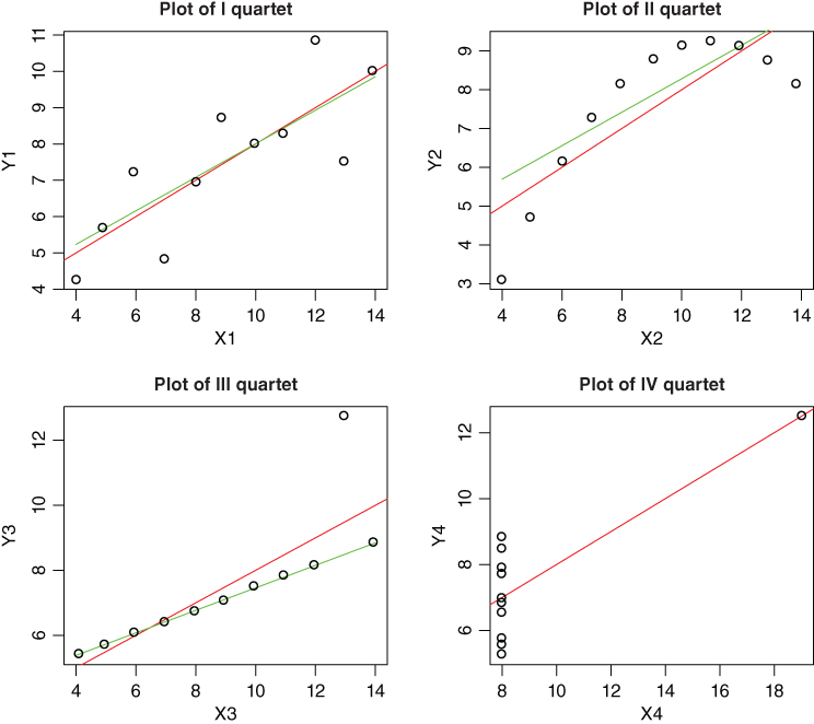
Figure 12.4 Regression and Resistant Lines for the Anscombe Quartet
We now fit and plot the resistant lines for the four quartets of this dataset. The regression lines are given in red and the resistant lines in green.
> attach(anscombe)
> rl1 <- resistant_line(x1,y1,iter=4); rl2 <- resistant_line(x2,y2, iter=4)
> rl3 <- resistant_line(x3,y3,iter=4); rl4 <- resistant_line(x4,y4, iter=4)
> par(mfrow=c(2,2))
> plot(x1,y1,main="Plot of I Quartet")
> abline(lm(y1∼x1,data=anscombe),col="red")
> curve(rl1$coeffs[1]+rl1$coeffs[2]*(x-rl1$xCenter),add=TRUE, col="green")
> plot(x2,y2,main="Plot of II Quartet")
> abline(lm(y2∼x2,data=anscombe),col="red")
> curve(rl2$coeffs[1]+rl2$coeffs[2]*(x-rl2$xCenter),add=TRUE, col="green")
> plot(x3,y3,main="Plot of III Quartet")
> abline(lm(y3∼x3,data=anscombe),col="red")
> curve(rl3$coeffs[1]+rl3$coeffs[2]*(x-rl3$xCenter),add=TRUE, col="green")
> plot(x4,y4,main="Plot of IV Quartet")
> abline(lm(y4∼x4,data=anscombe),col="red")
> curve(rl4$coeffs[1]+rl4$coeffs[2]*(x-rl4$xCenter),add=TRUE, col="green")
> rl1$coeffs
[1] 7.5447098 0.4617412
> rl2$coeffs
[1] 7.8525641 0.4315385
> rl3$coeffs
[1] 7.1143590 0.3461538
> rl4$coeffs
[1] NA NA
A very interesting thing happens in the fourth quartet. The slope has been computed as NA and the intercept is not available as a consequence of this. The reason is that 10 out of the 11 observations for the ![]() values are the same, and due to all the thirds of the
values are the same, and due to all the thirds of the ![]() 's being the same, the slope is given as
's being the same, the slope is given as NA. Figure 12.4 shows that resistant lines fit for each quartet of the Anscombe data. Also note that the slope and intercept values are estimated differently for each data set.
For more critical abuses of the linear regression model, especially in the context of multiple covariates, the reader should consult Box (1964).
12.4 Multiple Linear Regression Model
In Section 12.2 we considered the case of one predictor variable. If there is more than one predictor variable, say ![]() , we extend the simple regression model to the multiple linear regression model. Suppose that
, we extend the simple regression model to the multiple linear regression model. Suppose that ![]() is the variable of interest and that it is dependent on some covariates
is the variable of interest and that it is dependent on some covariates ![]() . The general linear regression model is given by
. The general linear regression model is given by
That is, the regressors are assumed to have a linear effect on the regressand. The vector ![]() is the vector of regression coefficients. The values of the
is the vector of regression coefficients. The values of the ![]() , are completely unspecified and take values on the real line. In a simple regression model, the regression coefficients have this interpretation: If the regressor
, are completely unspecified and take values on the real line. In a simple regression model, the regression coefficients have this interpretation: If the regressor ![]() , is changed by one unit while holding all other regressors at the same value, the change in the regressand
, is changed by one unit while holding all other regressors at the same value, the change in the regressand ![]() will be
will be ![]() .
.
For the ![]() individual in the study, the model is given by
individual in the study, the model is given by
The errors ![]() are assumed to be independent and identically distributed as the normal distribution
are assumed to be independent and identically distributed as the normal distribution ![]() with unknown variance
with unknown variance ![]() . We assume that we have a sample of size
. We assume that we have a sample of size ![]() . We will begin with the example of US crime data.
. We will begin with the example of US crime data.
12.4.1 Scatter Plots: A First Look
For the multiple regression data, let us use the R graphics method called pairs. The reader is recommended to try out the strength of this graphical utility with example(pairs). In a matrix of the scatter plot, a scatter plot is provided for each variable against the other variables. Thus, the output will be a symmetric matrix of scatter plots.
12.4.2 Other Useful Graphical Methods
The matrix of a scatter plot is a two-dimensional plot. However, we can also visualize scatter plots in three dimensions. Particularly, if we have two covariates and a regressand, the three-dimensional scatter plot comes in very handy for visualization purposes. The R package scatterplot3d may be used to visualize three-dimensional plots. We will consider the three-dimensional visualization of scatter plots in the next example. The discussion here is slightly varied in the sense that we do not consider a real dataset for obtaining the three-dimensional plots.
Contour plots are again useful techniques for understanding multivariate data through slices of the dataset. In continuation of the previous regression equations, from Example 13.4.3, let us view them in terms of a contour plot.
12.4.3 Fitting a Multiple Linear Regression Model
Given ![]() observations, the multiple linear regression model can be written in a matrix form as
observations, the multiple linear regression model can be written in a matrix form as
where ![]() ,
, ![]() , and
, and ![]() , and the covariate matrix
, and the covariate matrix ![]() 1 is
1 is

The least-squares normal equations for the multiple linear regression model is given by
which leads to the least-squares estimator
The model fitted values ![]() are obtained as
are obtained as
where we define
The matrix ![]() is called the hat matrix, which has many useful properties.
is called the hat matrix, which has many useful properties.
Properties of the Hat Matrix. The hat matrix is symmetric and idempotent, that is,
- 1.
 , symmetric property.
 - 2.
 , idempotent property.
 - 3. Furthermore,
 is also symmetric and idempotent.
The hat matrix plays a vital role in determining the residual values, which in turn is very useful in model adequacy, as will be seen in the Section 12.5. Chatterjee and Hadi (1988) refer to the hat matrix as the prediction matrix. The importance of the hat matrix is that it serves as a bridge between the observed values and the fitted values. By definition
We had seen earlier, in Section 12.2, the role of the residuals in estimation of the variance ![]() . The results further extend here in the following manner:
. The results further extend here in the following manner:

Thus, the residual mean square is
As in Section 12.2, ![]() is an unbiased estimator of
is an unbiased estimator of ![]() , that is,
, that is,
12.4.4 Testing Hypotheses and Confidence Intervals
12.4.4.1 Testing for Significance of the Regression Model
We need to first assert if the linear relationship between the regressand and the predictor variables is significant or not. In the terms of this hypothesis, this translates into testing for ![]() against the hypothesis
against the hypothesis ![]() for at least one
for at least one ![]() . Towards the problem of testing the hypotheses
. Towards the problem of testing the hypotheses ![]() against
against ![]() , we define the following:
, we define the following:
In Equation 12.42, we have ![]() . Computationally, we recognize that the regression sum of squares is obtained by exploiting the constraint
. Computationally, we recognize that the regression sum of squares is obtained by exploiting the constraint ![]() , that is by
, that is by ![]() . Under the hypothesis
. Under the hypothesis ![]() ,
, ![]() follows a
follows a ![]() distribution, and
distribution, and ![]() follows a
follows a ![]() distribution. Furthermore, it is noted that
distribution. Furthermore, it is noted that ![]() and
and ![]() are independent. Thus, the test statistic for the hypothesis
are independent. Thus, the test statistic for the hypothesis ![]() is the ratio of the mean of regression sum of squares to the mean of residual sum of squares, which is an
is the ratio of the mean of regression sum of squares to the mean of residual sum of squares, which is an ![]() -statistic. In summary, the test statistic is
-statistic. In summary, the test statistic is
which is an ![]() distribution. Now, to test
distribution. Now, to test ![]() , compute the test statistic
, compute the test statistic ![]() and reject it if
and reject it if
The ANOVA table is hence consolidated in Table 12.3.
Table 12.3 ANOVA Table for Multiple Linear Regression Model
| Source of Variation | Sum of Squares | Degrees of Freedom | Mean Square | |
| Regression | ||||
| Residual | ||||
| Total |
12.4.4.2 The Role of C Matrix for Testing the Regression Coefficients
The hypothesis ![]() tested above is a global test of model adequacy. If we reject the previous hypothesis, we may be interested in the specific predictors which are significant. Thus, there is a need to find such predictors.
tested above is a global test of model adequacy. If we reject the previous hypothesis, we may be interested in the specific predictors which are significant. Thus, there is a need to find such predictors.
The least-squares estimator ![]() is an unbiased estimator of
is an unbiased estimator of ![]() , and further
, and further
Define ![]() . Then the variance of the estimator of the
. Then the variance of the estimator of the ![]() regression coefficient
regression coefficient ![]() is
is ![]() , where
, where ![]() is the
is the ![]() diagonal element of the matrix
diagonal element of the matrix ![]() , and the covariance between
, and the covariance between ![]() and
and ![]() is
is ![]() .
.
We are now specifically interested in testing the hypothesis ![]() against the hypothesis
against the hypothesis ![]() ,
, ![]() . The test statistic for the hypothesis
. The test statistic for the hypothesis ![]() is
is

Under the hypothesis ![]() , the test statistic
, the test statistic ![]() follows a
follows a ![]() -distribution with
-distribution with ![]() degrees of freedom. Thus the test procedure is to reject the hypothesis
degrees of freedom. Thus the test procedure is to reject the hypothesis ![]() if
if ![]() .
.
Confidence Intervals
An important result, see Montgomery, et al. (2003), is the following:
This property allows us to construct the joint confidence region for the vector of regression coefficients ![]() as follows:
as follows:
The ![]() confidence intervals, region actually, for the regression coefficients is given by
confidence intervals, region actually, for the regression coefficients is given by
In the ![]() -dimensional space, the above inequality is a region of elliptical shape. As the next natural step, if we are interested in some specific predictor variable, the
-dimensional space, the above inequality is a region of elliptical shape. As the next natural step, if we are interested in some specific predictor variable, the ![]() confidence interval for its regression coefficient
confidence interval for its regression coefficient ![]() is given by
is given by
Finally, consider a new observation point ![]() . A natural estimate of the future observation
. A natural estimate of the future observation ![]() is
is ![]() . A
. A ![]() prediction interval is given as
prediction interval is given as
The theoretical developments for multiple linear regression model will now be taken to an R session.
The model validation task for the multiple linear regression model will be undertaken next.
12.5 Model Diagnostics for the Multiple Regression Model
In Sub-section 13.2.6 we saw the role of residuals for model validation. We have those and a few more options for obtaining residuals in the context of multiple regression. Cook and Weisberg (1982) is a detailed account of the role of residuals for the regression models.
Residuals may be developed in one of four ways:
- 1. Standardized residuals
- 2. Semi-Studentized residuals
- 3. Predicted Residuals, known by its famous abbreviation as PRESS
- 4. R-Student Residuals.
12.5.1 Residuals
Standardized Residuals. Scaling the residuals by dividing them by their estimated standard deviation, which is the square root of the mean residual sum of squares, we obtain the standardized residuals as
Note that the mean of the residuals is zero and in that sense it is present in the above expression. The standardized residuals ![]() are approximately standard normal variates, and any of their absolute values greater than 3 is an indicator of the presence of an outlier.
are approximately standard normal variates, and any of their absolute values greater than 3 is an indicator of the presence of an outlier.
Semi-Studentized Residuals. Recollect the definition of the hat matrix from Sub-section 13.4.3 and its usage to define the residuals as
Substituting ![]() , and on further evaluation, we arrive at
, and on further evaluation, we arrive at
Thus, the covariance matrix of the residuals is

The last step follows, since ![]() is an idempotent matrix. As the matrix
is an idempotent matrix. As the matrix ![]() is not necessarily a diagonal matrix, the residuals have different variances and are also correlated. Particularly, it can be shown that the variance of the residual
is not necessarily a diagonal matrix, the residuals have different variances and are also correlated. Particularly, it can be shown that the variance of the residual ![]() is
is
where ![]() is the
is the ![]() diagonal element of the hat matrix
diagonal element of the hat matrix ![]() . Furthermore, the covariance between the residuals
. Furthermore, the covariance between the residuals ![]() and
and ![]() is
is
where ![]() is the
is the ![]() diagonal element of the hat matrix. The semi-Studentized residuals are then defined as
diagonal element of the hat matrix. The semi-Studentized residuals are then defined as
PRESS Residuals. The PRESS residual, also called the predicted residual, denoted by ![]() , is based on a fit to data which does not include the
, is based on a fit to data which does not include the ![]() observation. Define
observation. Define ![]() as the least-squares estimate of the regression coefficients obtained by excluding the
as the least-squares estimate of the regression coefficients obtained by excluding the ![]() observation from the dataset. Then, the
observation from the dataset. Then, the ![]() predicted residual
predicted residual ![]() is defined by
is defined by
The picture looks a bit scary so that we may need to fit ![]() models to obtain the
models to obtain the ![]() predicted residuals. Even if we were willing to do this, for large
predicted residuals. Even if we were willing to do this, for large ![]() values, it may not be feasible to run the computer for so many hours, particularly if we can avoid it. There is an interesting relationship between the predicted residuals and the residuals, which circumvents the troublesome route of fitting
values, it may not be feasible to run the computer for so many hours, particularly if we can avoid it. There is an interesting relationship between the predicted residuals and the residuals, which circumvents the troublesome route of fitting ![]() models. Equation 2.2.23 of Cook and Weisberg (1982) shows that the predicted residuals and the residuals are related by
models. Equation 2.2.23 of Cook and Weisberg (1982) shows that the predicted residuals and the residuals are related by
The variance of the ![]() predicted residual is
predicted residual is
The standardized prediction residual, denoted by ![]() , is obtained by
, is obtained by
R-Student Residuals. Montgomery, et al. (2003) mention that the Studentized residuals are useful for outlier diagnostics and that the ![]() estimate of
estimate of ![]() is an internal scaling of the residual, since it is an internally generated estimate of
is an internal scaling of the residual, since it is an internally generated estimate of ![]() . Similar to the approach of prediction residual, we can construct an estimator of
. Similar to the approach of prediction residual, we can construct an estimator of ![]() by removing the
by removing the ![]() observation from the dataset. The estimator of
observation from the dataset. The estimator of ![]() by removing the
by removing the ![]() observation, denoted by
observation, denoted by ![]() , is computed by
, is computed by
Using ![]() for scaling purposes, the R-Student residual is defined by
for scaling purposes, the R-Student residual is defined by
The utility of these residuals is studied through the next example.
12.5.2 Influence and Leverage Diagnostics
In the previous subsection, we saw the power of leave-one-out residuals. The residual plots help in understanding the model adequacy. We will now take measures to explain the effect of each covariate on the model fit and also of each output value on the same.
A large value of residual may arise on account of either a large value of the covariate or a large value of the output. If some observations are disparagingly distinct from the overall dataset and if the reason for this is the covariate value, then such points are called the leverage points. The leverage points do not affect the estimates of the regression coefficients, although they are known to drastically change the ![]() values. For the fourth quartet of the Anscombe dataset, refer to the scatter plot in Figure 12.8, any value of the regressand should correspond to the covariate value of 8. Hence, we may say that the eighth observation is a levarage point.
values. For the fourth quartet of the Anscombe dataset, refer to the scatter plot in Figure 12.8, any value of the regressand should correspond to the covariate value of 8. Hence, we may say that the eighth observation is a levarage point.
Another source of disparaging observations, for reasonable levels of the covariate values, may be from the output values. Such data points are called influence points. The influence points have a significant affect on the estimated values of the regression coefficients, and in particular tilt the model relationship towards them. For the third quarter of the Anscombe dataset, refer to the scatter plot in Figure 12.8, the outliers are clearly influential.
Leverage Points
We will recollect the definition of the hat matrix:
The elements ![]() of the hat matrix may be interpreted as the amount of leverage exerted by the
of the hat matrix may be interpreted as the amount of leverage exerted by the ![]() observation
observation ![]() on the
on the ![]() fitted value
fitted value ![]() . Note that the diagonal elements may be easily obtained as
. Note that the diagonal elements may be easily obtained as
This hat matrix diagonal is a standardized measure of the distance of the ![]() observation from the center of the
observation from the center of the ![]() -space. The average size of a hat diagonal is
-space. The average size of a hat diagonal is ![]() . Any observation for which the
. Any observation for which the ![]() value exceeds twice the expected leverage of
value exceeds twice the expected leverage of ![]() is considered as a leverage point.
is considered as a leverage point.
Cook's Distance for the Influence Points
The Cook's distance for identifying the influence points is based on the leave-one-out approach as seen earlier. Let ![]() denote the
denote the ![]() fitted value, and
fitted value, and ![]() denote the
denote the ![]() predicted value when the
predicted value when the ![]() observation is removed from the model building, that is,
observation is removed from the model building, that is,
Then the Cook's distance for the ![]() observation is given by
observation is given by
The distance ![]() can be interpreted as the squared Euclidean distance that the vector of fitted values moves when the
can be interpreted as the squared Euclidean distance that the vector of fitted values moves when the ![]() observation is deleted. The magnitude of the distance
observation is deleted. The magnitude of the distance ![]() is assessed by comparing with
is assessed by comparing with ![]() . As a rule of thumb, any value of the distance
. As a rule of thumb, any value of the distance ![]() may be called an influential observation.
may be called an influential observation.
DFFITS and DFBETAS Measures for the Influence Points
To understand the influence of the ![]() observation on the regression coefficient
observation on the regression coefficient ![]() , the
, the ![]() measure proposed by Belsley, Kuh and Welsh (1980) is given as
measure proposed by Belsley, Kuh and Welsh (1980) is given as
where ![]() is the
is the ![]() diagonal element of the
diagonal element of the ![]() matrix, and
matrix, and ![]() is the estimate of the
is the estimate of the ![]() regression coefficient with the deletion of the
regression coefficient with the deletion of the ![]() observation. Belsley, Kuh, and Welsh suggest a cut-off value as
observation. Belsley, Kuh, and Welsh suggest a cut-off value as ![]() .
.
Similarly, a measure for understanding the affect of an observation on the fitted value is given by ![]() . This measure is defined as
. This measure is defined as
The relevant rule of thumb is a cut-off value of ![]() .
.
For a detailed list of R functions in the context of regression analysis, refer to the pdf file at http://cran.r-project.org/doc/contrib/Ricci-refcard-regression.pdf. The leverage points answer the problem of an outlier with respect to the covariate value. There may be at times linear dependencies among the covariates themselves, which lead to unstable estimates of the regression coefficients and this problem is known as the multicollinearity problem, which will be dealt with in the next section.
12.6 Multicollinearity
Multicollinearity is best understood by splitting its spelling as “multi-col-linearity”, implying a linear relationship among the multiple columns of the covariate matrix. In another sense, the columns of the covariate matrix are linearly dependent, and further it implies that the covariate matrix may not be of full rank. This linear dependence means that the covariates are strongly correlated. Highly correlated explanatory variables can cause several problems when applying the multiple regression model.
In general, we see that multicollinearity leads to the following problems:
- 1. Imprecise estimates of
 , that is, which also mislead the signs of the regression coefficients
 - 2. The
 -tests may fail to reveal significant factors
 - 3. Missing importance of predictors.
Spotting multicollinearity amongst a set of explanatory variables is a daunting task. The obvious course of action is to simply examine the correlations between these variables, and while this is often helpful, it is by no means foolproof, and more subtle forms of multicollinearity may be missed. An alternative and generally far more useful approach is to examine what are known as the variance inflation factors of the explanatory variables.
12.6.1 Variance Inflation Factor
The variance inflation factor ![]() for the
for the ![]() variable is given by
variable is given by
where ![]() is the square of the multiple correlation coefficient from the regression of the
is the square of the multiple correlation coefficient from the regression of the ![]() explanatory variable on the remaining explanatory variables. The variance inflation factor of an explanatory variable indicates the strength of the linear relationship between the variable and the remaining explanatory variables. A rough rule of thumb is that variance inflation factors greater than ten give cause for concern.
explanatory variable on the remaining explanatory variables. The variance inflation factor of an explanatory variable indicates the strength of the linear relationship between the variable and the remaining explanatory variables. A rough rule of thumb is that variance inflation factors greater than ten give cause for concern.
The eigen system analysis provides another approach to identify the presence of multicollinearity and will be considered in the next subsection.
12.6.2 Eigen System Analysis
Eigenvalues were introduced in Section 2.4. The eigenvalues of the matrix ![]() help to identify the multicollinearity effect in the data. Here, we need to standardize the matrix
help to identify the multicollinearity effect in the data. Here, we need to standardize the matrix ![]() in the sense that each column has a mean zero and standard deviation at 1. Suppose
in the sense that each column has a mean zero and standard deviation at 1. Suppose ![]() are eigenvalues of the matrix
are eigenvalues of the matrix ![]() . Let
. Let ![]() and
and ![]() . Define the condition number and condition indices of
. Define the condition number and condition indices of ![]() respectively by
respectively by
The multicollinearity problem is not an issue for the condition number less than 100, and moderate multicollinearity exists for the values of condition numbers in the range of 100 to 1000. If the condition number exceeds the large number of 1000, the problem of linear dependence among the covariates severely exists.Similarly, any condition index ![]() in excess of 1000 is an indicator of the almost linear-dependence of the covariates, and in general if the
in excess of 1000 is an indicator of the almost linear-dependence of the covariates, and in general if the ![]() condition indices are greater than 1000, we have
condition indices are greater than 1000, we have ![]() number of linear dependencies.
number of linear dependencies.
The decomposition of the matrix ![]() through the eigenvalues gives us the eigen system analysis in the sense that the matrix is decomposed with
through the eigenvalues gives us the eigen system analysis in the sense that the matrix is decomposed with
where ![]() is a
is a ![]() diagonal matrix with diagonal elements consisting of the eigenvalues of
diagonal matrix with diagonal elements consisting of the eigenvalues of ![]() and
and ![]() is a
is a ![]() orthogonal matrix whose columns consists of the eigenvectors of
orthogonal matrix whose columns consists of the eigenvectors of ![]() . If any of the eigenvalues is closer to zero, the corresponding eigenvector gives away the associated linear dependency. We will now continue to use these techniques on the US crime dataset.
. If any of the eigenvalues is closer to zero, the corresponding eigenvector gives away the associated linear dependency. We will now continue to use these techniques on the US crime dataset.
12.7 Data Transformations
In Chapter 4 we came across our first transformation technique through the concept of the rootogram. In regression analysis we need transformations for a host of reasons. A partial list of reasons is as follows:
- 1. The linearity assumption is violated, that is,
 may not be linear.
 - 2. For the variation in the
 's, the error variance may not be constant. This means that the variance of the
  's may be a function of the mean. In fact, the assumption of constant variance is also known as the assumption of homoscedasticity.
 - 3. Model errors do not follow a normal distribution.
- 4. In some experiments, we may have information about the need of transformations. For the model
 , the transformation
  provides us with a linear model. Such information may not be available a priori, and is reflected by residual plots only.
12.7.1 Linearization
As seen in the introduction, linearity is one of our basic assumptions. In many cases, it is possible to achieve linearity by an application of transformation. Many models which have non-linear terms may be transformed to a linear model by a suitable choice of transformation. See Table 6.1 of Chatterjee and Hadi (2006), or Table 5.1 of Montgomery, et al. (2003). For example, if we have the model ![]() , by using a log transformation, we obtain
, by using a log transformation, we obtain ![]() . The transformed model is linear in terms of its parameters. Figure 12.10 displays the behavior of
. The transformed model is linear in terms of its parameters. Figure 12.10 displays the behavior of ![]() for various choices of
for various choices of ![]() and
and ![]() (before the transformation).
(before the transformation).
> x <- seq(0,5,0.1)
> alpha <- 1
> par(mfrow=c(1,2))
> plot(x,y=alpha*xˆ{beta=1},xlab="x",ylab="y","l",lwd=1)
> points(x,y=alpha*xˆ{beta=0.5},"l",lwd=2)
> points(x,y=alpha*xˆ{beta=1.5},"l",lwd=3)
> points(x,y=alpha*xˆ{beta= -0.5},"b",lwd=2)
> points(x,y=alpha*xˆ{beta= -1},"b",lwd=3)
> points(x,y=alpha*xˆ{beta= -2},"b",lwd=2)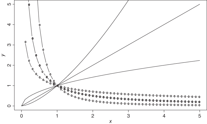
Figure 12.10 Illustration of Linear Transformation
We will next consider an example where a transformation achieves linearization.
12.7.2 Variance Stabilization
In general, the transformation stabilizes the variance of the error term. If the error variance is not constant for different ![]() values, we say that the error is heteroscedastic. The problem of heteroscedasticity is usually detected by the residual plots.
values, we say that the error is heteroscedastic. The problem of heteroscedasticity is usually detected by the residual plots.
Technically, we had built the model ![]() . The choice of transformation is not obvious. Moreover, it is difficult to say whether the power of
. The choice of transformation is not obvious. Moreover, it is difficult to say whether the power of ![]() is appropriate or some other positive number. Also, it is not always easy to choose between the power transformation and logarithmic transformation. A more generic approach will be considered in the next subsection.
is appropriate or some other positive number. Also, it is not always easy to choose between the power transformation and logarithmic transformation. A more generic approach will be considered in the next subsection.
12.7.3 Power Transformation
In the previous two subsections, we were helped by the logarithmic and square-root transformations. Box and Cox (1962) proposed a general transformation, called the power transformation. This method is useful when we do not have theoretical or empirical guidelines for an appropriate transformation. The Box-Cox transformation is given by

where ![]() . For details, refer to Section 5.4.1 of Montgomery, et al. (2003). The linear regression model that will be built is the following:
. For details, refer to Section 5.4.1 of Montgomery, et al. (2003). The linear regression model that will be built is the following:
For the choice of ![]() away from 0, we achieve variance stabilization, whereas for a value closer to 0, we obtain an approximate logarithmic transformation. The exact inference procedure for the choice of
away from 0, we achieve variance stabilization, whereas for a value closer to 0, we obtain an approximate logarithmic transformation. The exact inference procedure for the choice of ![]() cannot be taken up here, and we simply note that the MLE technique is used for this purpose.
cannot be taken up here, and we simply note that the MLE technique is used for this purpose.
12.8 Model Selection
Consider a linear regression model with ten covariates. The total number of possible models is then ![]() . The number of possible models is too enormous to investigate each one in depth. We also have further complications. Reconsider Example 12.4.5. It is seen from the output of the code
. The number of possible models is too enormous to investigate each one in depth. We also have further complications. Reconsider Example 12.4.5. It is seen from the output of the code summary(crime_rate_lm), that the variables S, Ex0, Ex1, LF, M, N, NW, U1, and W are all insignificant variables by their corresponding ![]() -value, as given in column
-value, as given in column Pr(>|t|). What do we do with such variables? If we have to discard them, what should be the procedure? For instance, it may be recalled from Example 12.6.1 that if the variable jitter(GBH) is dropped, the variable GBH will be significant. Hence, there is a possibility that if we drop one of the variables from crime_rate_lm, some other variable may turn out to be significant.
The need of model selection is thus more of a necessity than a fancy. Any text on regression models will invariably discuss this important technique. We will see the rationale behind it with an example.
A number of methods for model selection are available, including:
- Backward elimination
- Forward selection
- Stepwise regression.
12.8.1 Backward Elimination
The backward elimination method is the simplest of all variable selection procedures and can be easily implemented without a special function/package. In situations where there is a complex hierarchy, backward elimination can be run manually while taking account of what variables are eligible for removal. This method starts with a model containing all the explanatory variables and eliminates the variables one at a time, at each stage choosing the variable for exclusion as the one leading to the smallest decrease in the regression sum of squares. An ![]() -type statistic is used to judge when further exclusions would represent a significant deterioration in the model. The algorithm of backward selection is as follows:
-type statistic is used to judge when further exclusions would represent a significant deterioration in the model. The algorithm of backward selection is as follows:
- 1. Start with all the predictors in the model.
- 2. Remove the predictor with highest
 -value greater than
  critical.
 - 3. Refit the model and go to 2.
- 4. Stop when all
 -values are less than alpha critical.
The alpha critical is sometimes called the p-to-remove and does not have to be 5%. If prediction performance is the goal, then a 15 to 20% cut-off may work best, although methods designed more directly for optimal prediction should be preferred.
The above example is really taxing and there is a need to refine this before obtaining the final result. A customized R function which will achieve the same result is given next.
# The Backward Selection Methodology
pvalueslm <- function(lm) {summary(lm)$coefficients[,4]}
backwardlm <- function(lm,criticalalpha) {
 lm2 <- lm
 while(max(pvalueslm(lm2))>criticalalpha) {
 lm2 <- update(lm2,paste(".∼.-",attr(lm2$terms,"term.labels") [(which(pvalueslm(lm2)
              ==max(pvalueslm(lm2))))-1],sep=""))
 }
 return(lm2)
 }
12.8.2 Forward and Stepwise Selection
The forward selection method reverses the backward method. This method starts with a model containing none of the explanatory variables and then considers variables one by one for inclusion. At each step, the variable added is the one that results in the biggest increase in the regression sum of squares. An ![]() -type statistic is used to judge when further additions would not represent a significant improvement in the model.
-type statistic is used to judge when further additions would not represent a significant improvement in the model.
- 1. Start with no variables in the model.
- 2. For all predictors not in the model, check their
 -value if they are added to the model. Choose the one with lowest
  -value less than alpha critical.
 - 3. Continue until no new predictors can be added.
For a function similar to backwardlm, refer to Chapter 6 of Tattar (2013) for an implementation of the forward selection algorithm. Stepwise regression is a combination of forward selection and backward elimination. This addresses the situation where variables are added or removed early in the process and we want to change our mind about them later. Starting with no variables in the model, variables are added as with the forward selection method. Here, however, with each addition of a variable, a backward elimination process is considered to assess whether variables entered earlier might now be removed, because they no longer contribute significantly to the model.
We will now look at another criteria for model selection: Akaike Information Criteria, abbreviated as AIC. Let the log-likelihood function for a fitted regression model with ![]() covariates be denoted by
covariates be denoted by ![]() . The total number of estimated parameters is denoted by
. The total number of estimated parameters is denoted by ![]() . The AIC for the regression model is then given by
. The AIC for the regression model is then given by
where ![]() . The term
. The term ![]() is referred to as the penalty term. The model which has the least AIC value is considered the best model. For more details, refer to Sheather (2009). The use of AIC for forward and stepwise selection will be illustrated in the following.
is referred to as the penalty term. The model which has the least AIC value is considered the best model. For more details, refer to Sheather (2009). The use of AIC for forward and stepwise selection will be illustrated in the following.
12.9 Further Reading
In this section we consider some of the regression books which have been loosely classified into different sections.
12.9.1 Early Classics
Draper and Smith (1966–98) is a treatise on applied regression analysis. Chatterjee and Hadi (1977–2006) and Chatterjee and Hadi (1988) are two excellent companions for regression analysis. Bapat (2000) builds linear models using linear algebra and the book gives the reader an indepth knowledge of the necessary theory. Christensen (2011) develops a projective approach for linear models. For firm foundations in linear models, the reader may also use Rao, et al. (2008). Searle (1971) is a classic book, which is still preferred by some readers.
12.9.2 Industrial Applications
Montgomery, et al. (2003) and Kutner, et al. (2005) provide comprehensive coverages of linear models with dedicated emphasis on industrial applications.
12.9.3 Regression Details
Belsley, Kuh and Welsh (1980), Fox (1991), Cook (1998), Cook and Weisberg (1982), Cook and Weisberg (1994), and Cook and Weisberg (1999) are the monographs which have details about regression diagnostics. For a robust regression model, the reader will find a very useful source in Rousseeuw and Leroy (1987).
12.9.4 Modern Regression Texts
Andersen and Skovgaard (2010) consider many variants of regression models which have linear predictors. Gelman and Hill (2007) develop hierarchical regression models. Freedman (2009) is an instant classic which lays more emphasis on matrix algebra. Sengupta and Rao (2003), Clarke (2008), Seber and Lee (2003), and Rencher and Schaalje (2008) are also useful accounts of the linear models.
12.9.5 R for Regression
Fox (2002) is an early text on the use of R software for regression analysis. Faraway (2002) is an open source book which has detailed R programs for linear models.
12.10 Complements, Problems, and Programs
Problem 12.1 Fit a simple linear regression model for the Galton dataset as seen in Example 4.5.1. Compare the values of the regression coefficients of the linear regression model for this dataset with the previously obtained resistant linecoefficients.
Problem 12.2 Verify that Equation 12.19 is satisfied for Example 13.2.3. Fit the resistant lines model for this dataset, and verify whether the ANOVA decomposition holds for the fitted values obtained using the resistant line model.
Problem 12.3 Extend the concept of
 and
and  for the resistant line model. Create an R function which will extract these two measures for a fitter resistant line model and obtain these values for the Galton dataset,
 rp, andtc.Problem 12.4 The
Signif. codesas obtained bysummary(lm)may be easily customized in R to use your own cut-off points, and symbols too. There are two elements to this, first the cut-off points for the -values and the default settings are
 cutpoints = c(0, 0.001, 0.01, 0.05, 0.1, 1), and the second part has the symbols insymbols = c(“***”, “**”, “*”, “.”, “ ”). Change these default settings to, say,symbols = c(“$$$”, “$$”, “$”, “.”, “ ”)by first runningfix(printCoefmat). Edit theprintCoefmatand save it. The changes in this object are then applied in an R session by running the codeassignInNamespace(“printCoefmat”, printCoefmat, “stats”)at the console. Customize yourSignif. codesand complete the program!Problem 12.5 The model validation in Example 13.2.6 for the Toluca Company dataset has been carried out using the residuals. The semi-Studentized residuals also play a critical role in determining departures from the assumptions of the linear regression model. Obtain the six plots as in that example with the semi-Studentized residuals.
Problem 12.6 The model validation aspects need to be checked for the Rocket propellant problem, Example 13.2.1. Complete the program for the fitted simple linear regression model and draw the appropriate conclusions.
Problem 12.7 In Example 13.4.3, change the range of the variables
x1andx2tox1 <- rep(seq(-10,10,0.5),100)andx2 <- rep(seq(-10,10,0.5),each=100)and redo the three-dimensional plot, especially for the third linear regression model. Similarly, for the contour plot of the same model, change the variable ranges tox1=x2=seq(from=-5,to=5,by=0.2)and redraw the contour plot. What are your typical observations?Problem 12.8 For the fitted linear model
crime_rate_lm, using theuscdataset, obtain the plot of residuals against the fitted values.Problem 12.9 Verify the properties of the hat matrix
 given in Equation 12.37 for the fitted object
 crime_rate_lm, or any other fitted multiple linear regression model of your choice.Problem 12.10 Using self-defined functions for
 and
and  , as given in Equations 12.66 and 12.65, say
 my_dffitsandmy_dfbetas, compute the values for anailmfitted object and compare the results with the R functionsdffitsanddfbetas.Problem 12.11 The VIF given in Equation 12.67 for a covariate requires computation of
 , as obtained in the regression model when the covariate is an output and other covariates are input variables for it. Thus, using
 1/(1-summary(lm(xi∼x1+...+xi-1+xi+1+...+xp))$r.squared), the VIF of the covariate may be obtained. Verify the VIFs obtained in Example 13.6.2.
Problem 12.12 Identify if the multicollinearity problems exist for the fitted
ailmobject using (i) VIF method, and (ii) eigen system analysis.Problem 12.13 Carry out the Box-Cox transformation method for the
bacteria_studyand compare it with the result in Example 13.7.1 of the log transformation technique,bacterialoglm.Problem 12.14 For the prostate cancer problem discussed in Example 13.8.1, find the best possible linear regression model using (i) step-wise, (ii) forward, and (iii) backward selection technique.