Chapter 17
Generalized Linear Models
Package(s): gdata, RSADBE
Dataset(s): chdage, lowbwt, sat, Disease, BS, caesareans
17.1 Introduction
In Chapter 16 we discussed many useful statistical methods for analysis of categorical data, which may be nominal or ordinal data. The related regression problems were deliberately not touched upon there, the reason for omission being that the topic is more appropriate here. We will see in the next section that the linear regression methods of Chapter 12 are not appropriate for explaining the relationship between the regressors and discrete regressands. The statistical models, which are more suitable for addressing this problem, are known as the generalized linear models, which we abbreviate to GLM.
In this chapter, we will consider the three families of the GLM: logistic, probit, and log-linear models. The logistic regression model will be covered in more detail, and the applications of the others will be clearly brought out in the rest of this chapter.
We first begin with the problem of using the linear regression model for count/discrete data in Section 17.2. The exponential family continues to provide excellent theoretical properties for GLMs and the relationship will be brought out in Section 17.3. The important logistic regression model will be introduced in Section 17.4. The statistical inference aspects of the logistic regression model is developed and illustrated in Section 17.5. Similar to the linear regression model, we will consider the similar problem of model selection in Section 17.6. Probit and Poisson regression models are developed in Sections 17.7 and 17.8.
17.2 Regression Problems in Count/Discrete Data
By count/discrete data, we refer to the case where the regressand/output is discrete. That is, the output ![]() takes values in the set
takes values in the set ![]() , or
, or ![]() . As in the case of the linear regression model, we have some explanatory variables which effect the output
. As in the case of the linear regression model, we have some explanatory variables which effect the output ![]() . we will immediately see the shortcomings of the approach of the linear regression model.
. we will immediately see the shortcomings of the approach of the linear regression model.
we will now digress a bit from applications and attempt to understand the general underlying theory of GLMs. A brief look at the important members of the GLM family will be discussed here.
17.3 Exponential Family and the GLM
The exponential family of distribution was introduced in Chapter 7. Chapter 3 of Dobson (2002) highlights the role of the exponential family for the GLM's considered in this chapter. Recall the definition of the exponential family from Chapter 7 as
where ![]() are some known functions. This form of exponential family may be rewritten as
are some known functions. This form of exponential family may be rewritten as
where ![]() and
and ![]() . If
. If ![]() , the distribution is said to be in canonical form and in this case
, the distribution is said to be in canonical form and in this case ![]() is called the natural parameter of the distribution. we had seen some members of the exponential family in Section 7.2.1. The dependency of GLM on the exponential family is now discussed.
is called the natural parameter of the distribution. we had seen some members of the exponential family in Section 7.2.1. The dependency of GLM on the exponential family is now discussed.
Consider an independent sample ![]() , with the following characteristics:
, with the following characteristics:
- Each observation
 , is a distribution from the exponential family.
 - The distributions of
 are of the same form, that is, all are either normal, or all binomial, etc.
 - The canonical form
 is specified by
17.1
is specified by
17.1
This translates into the form that the joint probability density function of the random sample
 , is given by17.2
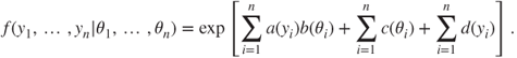
In a GLM, we are interested in estimation of the ![]() parameters
parameters ![]() . The trick is to consider some function of
. The trick is to consider some function of ![]() , say
, say ![]() , such that
, such that ![]() , and then allow the
, and then allow the ![]()
![]() 's to vary as a function of
's to vary as a function of ![]() , regression coefficients. That is, we define
, regression coefficients. That is, we define ![]() by
by
where ![]() is the covariate vector associated with
is the covariate vector associated with ![]() . The function
. The function ![]() is called the link function of the GLM. Some essential requirements of the function
is called the link function of the GLM. Some essential requirements of the function ![]() is that it should be monotonic and differentiable. Table 17.1 gives a summary of important members of the GLM. There will be more focus on logistic regression in this chapter.
is that it should be monotonic and differentiable. Table 17.1 gives a summary of important members of the GLM. There will be more focus on logistic regression in this chapter.
Table 17.1 GLM and the Exponential Family
| Probability Model | Name of Link Function | Link Function | Mean Function |
| Normal | Identity | ||
| Exponential/Gamma | Inverse | ||
| Inverse Gaussian | Inverse Squared | ||
| Poisson | Log | ||
| Binomial | Logit |
17.4 The Logistic Regression Model
We saw in the previous section how the probability curve is a sigmoid curve. Now we will introduce the concepts in a more formal and mathematical way. We have found the paper of Czepiel, http://czep.net/stat/mlelr.pdf, to be in the most appropriate pedagogical manner and this section is a liberal adaptation of the same. Let the binary outcomes be represented by ![]() , and the covariates associated with them be respectively
, and the covariates associated with them be respectively ![]() . The covariate is assumed to be a vector of the
. The covariate is assumed to be a vector of the ![]() elements, that is,
elements, that is, ![]() . Without loss of generality, we can write the covariate vector as
. Without loss of generality, we can write the covariate vector as ![]() , with
, with ![]() . The probability of success is specified by
. The probability of success is specified by ![]() . The logistic regression model is then given by
. The logistic regression model is then given by

where ![]() is the vector of regression coefficients. The probability of a failure has the simple form:
is the vector of regression coefficients. The probability of a failure has the simple form:
An important identity in the context of logistic regression is the form of the odds ratio, abbreviated and denoted as OR:
Taking the logarithm on both sides of the above equation, we get the form of logistic regression model:

The expression ![]() is known as the logit function and since it is linear in the covariates, the logistic regression model, based on the logit function, is a particular class of the well-known generalized linear models. The logistic regression model is given by
is known as the logit function and since it is linear in the covariates, the logistic regression model, based on the logit function, is a particular class of the well-known generalized linear models. The logistic regression model is given by
where ![]() is the error term. Thus, if
is the error term. Thus, if ![]() , the error is
, the error is ![]() with probability
with probability ![]() . Otherwise, the error is
. Otherwise, the error is ![]() with probability
with probability ![]() . That is
. That is
Hence, the error ![]() has a binomial distribution with mean
has a binomial distribution with mean ![]() and variance
and variance ![]() . The next section will deal with the inferential aspect of
. The next section will deal with the inferential aspect of ![]() .
.
17.5 Inference for the Logistic Regression Model
17.5.1 Estimation of the Regression Coefficients and Related Parameters
The likelihood function based on ![]() observations is given by
observations is given by
As in the most cases, it is easier to work with the log-likelihood function:
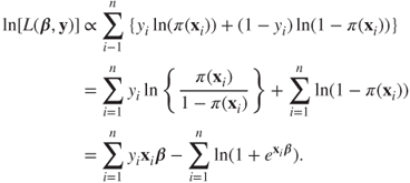
Differentiating the above log-likelihood function with respect to ![]() , we obtain the score function:
, we obtain the score function:

Let us denote the covariate matrix, as in earlier chapters, by ![]() , the probability of success vector by
, the probability of success vector by ![]() , and the outcome vector by
, and the outcome vector by ![]() . The normal equation, obtained by equating the above equation to zero, for the logistic regression model is then given by
. The normal equation, obtained by equating the above equation to zero, for the logistic regression model is then given by
The above equation looks similar to the normal equation of the linear models. However, Equation 17.11 cannot be solved immediately as the vector ![]() contains the vector of regression coefficients. We need the help of a different algorithm to obtain the estimates of the regression coefficients. This algorithm is generally known as the iterated reweighted least squares, abbreviated as IRLS, algorithm. In the context of the logistic regression model, the IRLS algorithm is given below, see Fox http://socserv.mcmaster.ca/jfox/Courses/UCLA/logistic-regression-notes.pdf.
contains the vector of regression coefficients. We need the help of a different algorithm to obtain the estimates of the regression coefficients. This algorithm is generally known as the iterated reweighted least squares, abbreviated as IRLS, algorithm. In the context of the logistic regression model, the IRLS algorithm is given below, see Fox http://socserv.mcmaster.ca/jfox/Courses/UCLA/logistic-regression-notes.pdf.
- Initialize the vector of regression coefficients
 .
. - The
 improvement of the regression coefficients is given by
where
 is a diagonal matrix with the
  diagonal element given by
  , and
, and  .
. - Repeat the above step until
 is close to
  .
. - The asymptotic covariance matrix of the regression coefficients is given by
 , see next sub-section.
In the next example, we will develop an example which will clearly bring out the steps of the IRLS algorithm. The use of the R function glm directly returns us the estimates of the regression coefficients. However, the working of the IRLS algorithm does not become clear, and the first time the reader may feel that IRLS is some kind of black box. It is to be understood that software does not hide anything, R or any other statistical software. The onus of clear understanding of software functionality is with the reader, and sometimes the authors. For the sake of simplicity, we will focus on the simple GLM case of a single covariate only. The IRLS function is first given and discussed.
irls <- function(output, input) {
input <- cbind(rep(1,length(output)),input)
bt <- 1:ncol(input)*0 # Initializing the regression coefficients
probs <- as.vector(1/(1+exp(-input%*%bt)))
temp <- rep(1,nrow(input))
while(sum((bt-temp)ˆ2)>0.0001) {
temp <- bt
bt <- bt+as.vector(solve(t(input)%*%diag(probs*(1-probs))
%*%input)%*%(t(input)%*%(output-probs)))
probs <- as.vector(1/(1+exp(-input%*%bt)))
}
return(bt)
}
The irls R function defined here should return us the estimates as required by the IRLS algorithm and in particular Equation 17.12 computations are to be handled here. Given the covariate values for the ![]() observations from a dataset, the first step is to take care of the intercept term, and thus we first begin by inserting a column of 1's with
observations from a dataset, the first step is to take care of the intercept term, and thus we first begin by inserting a column of 1's with input <- cbind(rep(1,length(output)),input). The initial estimate of regression coefficients is set equal to 0, and hence the initial probabilities ![]() 's will be zero too, see
's will be zero too, see bt and probs in the irls program. The regression coefficient vector for the previous iteration will be denoted by temp and so long as the improvement of the current iteration, vector distance, and the previous iteration is greater than 1e-4, the iterations will be carried out in the while loop. The iteration as required by Equation 17.12 is provided by the R code solve(t(input)%*%diag(probs*(1-probs))%*%input)%*%(t(input) %*%(output-probs)). When the convergence criteria is met, the vector of regression coefficients is returned by return(bt) as the output. The irls function will be tested for the coronary heart disease problem and the results will be further verified with the R glm function.
Estimates of the link function and odds ratio is straightforwardly obtained by plugging in the values of the estimated regression coefficients, that is,

We will next consider an example of the multiple logistic regression, that is when we have more than one covariates.
The estimated vector of regression coefficients ![]() needs to be tested for significance. The first step towards this would be to obtain an estimate of the variance-covariance matrix of
needs to be tested for significance. The first step towards this would be to obtain an estimate of the variance-covariance matrix of ![]() .
.
17.5.2 Estimation of the Variance-Covariance Matrix of 
We have seen earlier in Chapter 7 that the variance of the score function gives the Fisher information. Thus, to obtain the variance-covariance matrix of ![]() , we look at the second-order partial derivatives of the log-likelihood function. The technique of estimating the variance-covariance matrix of
, we look at the second-order partial derivatives of the log-likelihood function. The technique of estimating the variance-covariance matrix of ![]() follows from the theory of the maximum likelihood estimation, see Rao (1973). Differentiating the partial differential equations of the log-likelihood function of sub-section 8.4.1, we get
follows from the theory of the maximum likelihood estimation, see Rao (1973). Differentiating the partial differential equations of the log-likelihood function of sub-section 8.4.1, we get
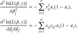
for ![]() . The Fisher information for
. The Fisher information for ![]() , denoted by
, denoted by ![]() , consists of elements as specified in the above two equations. Adapting the results from Chapter 7, the inverse matrix of the information matrix gives us the variance-covariance matrix of
, consists of elements as specified in the above two equations. Adapting the results from Chapter 7, the inverse matrix of the information matrix gives us the variance-covariance matrix of ![]() , that is,
, that is,
Thus, we specifically have that the variance of the estimator of regression coefficient ![]() , denoted by
, denoted by ![]() as the
as the ![]() diagonal element of
diagonal element of ![]() . Similarly, the covariance between the estimators of two regression coefficients, denoted by
. Similarly, the covariance between the estimators of two regression coefficients, denoted by ![]() , as the
, as the ![]() element of
element of ![]() .
.
In R, it is easier to obtain the variance-covariance matrix for a fitted logistic regression model. For the Low Birth-Weight example, we can obtain this using the listed object cov.unscaled.
> lowglm_summary <- summary(lowglm)
> lowglm_summary$cov.unscaled
            (Intercept)     AGE     LWT   RACE2   RACE3     FTV
(Intercept)      1.1480 -0.0220 -0.0045 -0.0373 -0.1339  0.0054
AGE             -0.0220  0.0011  0.0000  0.0031  0.0013 -0.0010
LWT             -0.0045  0.0000  0.0000 -0.0008  0.0003 -0.0001
RACE2           -0.0373  0.0031 -0.0008  0.2479  0.0571 -0.0003
RACE3           -0.1339  0.0013  0.0003  0.0571  0.1312  0.0058
FTV              0.0054 -0.0010 -0.0001 -0.0003  0.0058  0.0280
17.5.3 Confidence Intervals and Hypotheses Testing for the Regression Coefficients
The natural hypotheses testing problem is inspection for the significance of the regressors, that is, ![]() . The Wald test statistics for
. The Wald test statistics for ![]() is given by
is given by
Under the hypotheses ![]() , the Wald statistics
, the Wald statistics ![]() (asymptotically) follow a standard normal distribution. Furthermore, the
(asymptotically) follow a standard normal distribution. Furthermore, the ![]() confidence interval for
confidence interval for ![]() is given by
is given by
We will illustrate these concepts for the low birth-weight study problem.
An overall model level significance test needs to be in place. Towards this test, we need to first define the notion of deviance, and this topic will be taken up in sub-section 17.5.5. First, we need to define the various types of residuals on the lines of linear models for the logistic regression model.
17.5.4 Residuals for the Logistic Regression Model
Recollect from the definition of residuals for the linear regression model as defined in Section 12.5 that the residual is the difference between actual and predicted ![]() values. Similarly, the residuals for the logistic regression model is defined by
values. Similarly, the residuals for the logistic regression model is defined by
The residuals ![]() are sometimes called the response residual. The different variants of the residuals which will be useful are defined next, see Chapter 7 of Tattar (2013). The hat matrix
are sometimes called the response residual. The different variants of the residuals which will be useful are defined next, see Chapter 7 of Tattar (2013). The hat matrix ![]() played an important role in defining the residuals for the linear regression model, recall Equation (12.37). A similar matrix will be required for the logistic regression model, and we have the problem here that the observation
played an important role in defining the residuals for the linear regression model, recall Equation (12.37). A similar matrix will be required for the logistic regression model, and we have the problem here that the observation ![]() is not a straightforward linear in terms of the regression coefficient. A linear approximation for the fitted values
is not a straightforward linear in terms of the regression coefficient. A linear approximation for the fitted values ![]() , which gives a similar hat matrix for the logistic regression model, has been proposed by Pregibon (1981), see Section 5.3 of Hosmer and Lemeshow (1990–2013). The hat matrix for the logistic regression matrix will be denoted by
, which gives a similar hat matrix for the logistic regression model, has been proposed by Pregibon (1981), see Section 5.3 of Hosmer and Lemeshow (1990–2013). The hat matrix for the logistic regression matrix will be denoted by ![]() , the subscript
, the subscript ![]() denotes logistic regression and not linear regression, and is defined by
denotes logistic regression and not linear regression, and is defined by
where ![]() is a diagonal matrix with
is a diagonal matrix with
The diagonal elements, hat values, ![]() , or simply
, or simply ![]() , are given by
, are given by
with ![]() capturing the model-based estimator of the variance of
capturing the model-based estimator of the variance of ![]() and
and ![]() computing the weighted distance of
computing the weighted distance of ![]() from the average of the covariate design matrix
from the average of the covariate design matrix ![]() . Similar to the linear regression model case, the diagonal element
. Similar to the linear regression model case, the diagonal element ![]() is useful for obtaining the variance of the residual:
is useful for obtaining the variance of the residual:
The Pearson residual for the logistic regression model is then defined by
The standardized Pearson residual is defined by

The deviance residual for the logistic regression model is defined as signed square root of the contribution of the observation to the sum of the model deviance and is given by
The residuals are obtained for a disease outbreak dataset, which is adapted from Kutner, et al. (2005).
Recollect from Equation 17.7 that the mean and variance of the error term are respectively ![]() and
and ![]() . Thus, the LOESS plot, refer to Section 8.4, of errors against the fitted values should reflect a line around 0 if the assumption of the logistic regression is appropriate. This perspective will be explored as a continuation of the previous example.
. Thus, the LOESS plot, refer to Section 8.4, of errors against the fitted values should reflect a line around 0 if the assumption of the logistic regression is appropriate. This perspective will be explored as a continuation of the previous example.
The residuals have more importance than validation of the model assumptions. The overall fit of the model will be investigated next.
17.5.5 Deviance Test and Hosmer-Lemeshow Goodness-of-Fit Test
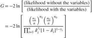
Testing for the significance of the GLM model is carried out using Deviance Statistic, denoted by ![]() , by comparing the likelihood function for the fitted model, which includes the covariates, with the likelihood of the saturated model. A saturated model is that model which takes into consideration all possible parameters and thus results in a perfect fit in the sense that all successful outcomes are predicted as success and failures predicted as failed. The deviance statistic
, by comparing the likelihood function for the fitted model, which includes the covariates, with the likelihood of the saturated model. A saturated model is that model which takes into consideration all possible parameters and thus results in a perfect fit in the sense that all successful outcomes are predicted as success and failures predicted as failed. The deviance statistic ![]() is then defined by
is then defined by
Since the saturated model, by definition, leads to a perfect fit, we have ![]() , and thus
, and thus
Thus, the deviance statistic becomes

To know the significance of the set of the independent variables, we need to compare the value of ![]() with and without the set of independent variables/covariates. That is
with and without the set of independent variables/covariates. That is
We further see that
where ![]() and
and ![]() . Basically, we are substituting the MLEs of
. Basically, we are substituting the MLEs of ![]() and
and ![]() for the model without the set of independent variables. Under the hypothesis that all the regression coefficients are not significant, the test statistic
for the model without the set of independent variables. Under the hypothesis that all the regression coefficients are not significant, the test statistic ![]() follows a
follows a ![]() - distribution with
- distribution with ![]() degrees of freedom. With the appropriate significance level, it is possible to infer the model significance using the
degrees of freedom. With the appropriate significance level, it is possible to infer the model significance using the ![]() statistic. This
statistic. This ![]() statistic may be seen as the parallel of the
statistic may be seen as the parallel of the ![]() statistic in the linear model case. For more details, refer to Hosmer and Lemeshow (2000).
statistic in the linear model case. For more details, refer to Hosmer and Lemeshow (2000).
17.6 Model Selection in Logistic Regression Models
We consider “Stepwise Logistic Regression” for the best variable selection in a logistic regression model. The most important variable is the one that produces maximum change in the log-likelihood relative to a model containing no variables. That is, maximum change in the value of the ![]() -statistic is considered as the most important variable. The complete process of step-wise logistic regression is given in S number of steps.
-statistic is considered as the most important variable. The complete process of step-wise logistic regression is given in S number of steps.
Step 0
- Consider all plausible variables, say
 .
. - Fit “intercept only model”, and evaluate the log-likelihood
 .
. - Fit each of the possible
 univariate logistic regression models and note the log-likelihood values
  . Furthermore, calculate the
  -statistic for each of the
  -models,
  .
. - Obtain the
 -value for each model.
 - The most important variable is then the one with least
 -value,
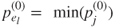
- Denote the most important variable by
 .
. - Define the entry criteria
 -value as
  , which will at any time throughout this procedure decide if the variable is to be included or not. That is, the variable with the least
  -value must be less than
  to be selected in the final model.
 - If none of the variables have the
 -value less than
  , we stop.
Step 1. The Forward Selection Step
- Replace
 of the previous step with
  .
. - Fit
 models with variables
  and the remaining variables
  ,
,  , and
, and  distinct from
  .
. - For each of the
 models, calculate the log-likelihood
  and the
  -statistics
 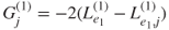 , and the corresponding
  -values, denoted
  .
. - Define

- If
 , stop.
Step 2A. The Backward Elimination Step
- Adding
 may leave
  statistically insignificant.
 - Let
 denote the log-likelihood of the model with variable
  removed.
 - Calculate the likelihood-ratio test of these reduced models with respect to the full model at the beginning of this step
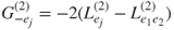 , and calculate the
  -values
  .
. - Deleted variables must result in a maximum
 -value of the modified model.
 - Denote
 as the variable which is to be removed, and define
  .
. - To remove variables, we need to have a value
 with respect to which we compare
  .
. - We need to have
 . (Why?)
 - Variables are removed if
 .
.
Step 2B. The Forward Selection Phase
- Continue the forward selection method with
 remaining variables and find
  .
. - Let
 be the variable associated with
  .
. - If the
 is less than
  , proceed to Step 3, otherwise stop.
Step 3
- Fit the model including the variable selected in the previous step and perform backward elimination and then forward selection phase.
- Repeat until the last Step S.
Step S
- Stopping happens if all the variables have been selected in the model.
- It also happens if all the
 -values in the model are less than
  , and the remaining variables have
  -values exceeding
  .
.
The step function in R may be used to build a model. The criteria used there is the Akaike Information Criteria, AIC. To the best of our knowledge, there is no package/function which will implement stepwise logistic regression using the ![]() -statistic generated
-statistic generated ![]() -values. The Hosmer and Lemeshow (2000) approach of model selection will be used here.
-values. The Hosmer and Lemeshow (2000) approach of model selection will be used here.
We will next illustrate the concept of the backward regression selection method using the AIC criteria.
An alternative to the binary regression problem, as discussed here with the logistic regression model, is given by the probit model and we will discuss this in the next section.
17.7 Probit Regression
Bliss (1935) proposed the use of the probit regression model for problems where the response variable is a binary variable. Recall that in the logistic regression model we used the logit transformation of the link function to ensure that the predicted probabilities were always in the unit interval. Bliss suggested modeling the link function using the normal cumulative distribution.
Let ![]() denote the binary outcome as earlier and the covariates be represented by
denote the binary outcome as earlier and the covariates be represented by ![]() . The probit regression model is constructed through the use of an auxiliary RV denoted by
. The probit regression model is constructed through the use of an auxiliary RV denoted by ![]() , see Chapter 7 of Tattar (2013). The auxiliary RV
, see Chapter 7 of Tattar (2013). The auxiliary RV ![]() is then modeled as the multiple linear regression model:
is then modeled as the multiple linear regression model:
where the error ![]() follows the normal distribution
follows the normal distribution ![]() . Without loss of generality we assume
. Without loss of generality we assume ![]() . The vectors
. The vectors ![]() and
and ![]() have their usual meanings. The probit regression model is then developed as a latent variable model through the use of the auxiliary RV:
have their usual meanings. The probit regression model is then developed as a latent variable model through the use of the auxiliary RV:
The probit model is then given by
where ![]() denotes the cumulative distribution of a standard normal variable. If we have
denotes the cumulative distribution of a standard normal variable. If we have ![]() pairs of observations
pairs of observations ![]() , the statistical inference for
, the statistical inference for ![]() may be carried out through the likelihood function given by
may be carried out through the likelihood function given by
It is obvious that this likelihood function will be difficult to evaluate. A probit regression model is set up in R, again using the glm function with the option binomial(probit). Since the fitted probit model is again a member of the glm class, the techniques available and discussed for the logistic regression model are also available for the fitted probit model. For the sake of paucity, the mathematical details of the probit model will be skipped. First, we consider the simple probit model, followed with an example of multiple probit model.
A lot of similarity exists between the logistic regression and the probit regression regarding the model building in R, since both are generated using the glm function. Especially, the computational and inference methods remain almost the same. We will close this section with an illustration of the step-wise regression method for the probit regression model.
The next section will deal with a different type of discrete variable.
17.8 Poisson Regression Model
The logistic and probit regression models are useful when the discrete output is a binary variable. By an extension, we can incorporate multi-nominal variables too. However, these variables are class indicators, or nominal variables. In Section 16.5, the role of the Poisson RV was briefly indicated in the context of discrete data. If the discrete output is of a quantitative type and there are covariates related to it, we need to use the Poisson regression model.
The Poisson regression models are useful in two slightly different contexts: (i) the events arising as a percentage of the exposures, along with covariates which may be continuous or categorical, and (ii) the exposure effect is constant with the covariates being categorical variables only. In the first type of modeling, the parameter (rate ![]() ) of the Poisson RV is specified in terms of the units of exposure. As an example, the quantitative variable may refer to the number of accidents per thousand vehicles arriving at a traffic signal, or the number of successful sales per thousand visitors on a web page. In the second case, the regressand
) of the Poisson RV is specified in terms of the units of exposure. As an example, the quantitative variable may refer to the number of accidents per thousand vehicles arriving at a traffic signal, or the number of successful sales per thousand visitors on a web page. In the second case, the regressand ![]() may refer to the count in each cell of a contingency table. The Poisson model in this case is popularly referred to as the log-linear model. For a detailed treatment of this model, refer to Chapter 9 of Dobson (2002).
may refer to the count in each cell of a contingency table. The Poisson model in this case is popularly referred to as the log-linear model. For a detailed treatment of this model, refer to Chapter 9 of Dobson (2002).
Let ![]() denote the number of responses from
denote the number of responses from ![]() events for the
events for the ![]() exposure,
exposure, ![]() , and let
, and let ![]() represent the vector of explanatory variables. The Poisson regression model is stated as
represent the vector of explanatory variables. The Poisson regression model is stated as
Here, the natural link function is the logarithmic function
The extra term ![]() that appears in the link function is referred to as the offset term. It is important to clearly specify here the form of the pmf of
that appears in the link function is referred to as the offset term. It is important to clearly specify here the form of the pmf of ![]() :
:
The likelihood function is then given by

The (ML) technique of obtaining ![]() is again based on the IRLS algorithm. However, this aspect will not be dealt with here. It is assumed that the ML estimate is available for
is again based on the IRLS algorithm. However, this aspect will not be dealt with here. It is assumed that the ML estimate is available for ![]() , as returned by say R software, and by using it we will then look at other aspects of the model. The fitted values from the Poisson regression model are given by
, as returned by say R software, and by using it we will then look at other aspects of the model. The fitted values from the Poisson regression model are given by
and hence the residuals are
Note that the mean and variance of the Poisson model are equal, and hence an estimate of the variance of the residual is ![]() , which leads to the Pearson residuals:
, which leads to the Pearson residuals:
A ![]() goodness-of-fit test statistic is then given by
goodness-of-fit test statistic is then given by
These concepts will be demonstrated through the next example.
For a binary regressand, we can obtain a precise answer for the influence of the variable on the rate of the Poisson model through the concept of the rate ratio. The rate ratio, denoted by RR, gives the impact of the variable on the rate, by looking at the ratio of the expected value of ![]() , when the variable is present to the expected value when it is absent:
, when the variable is present to the expected value when it is absent:
If the RR value is closer to unity, it implies that the indicator variable has no influence on ![]() . The confidence intervals, based on the invariance principle of MLE, is obtained with a simple exponentiation of the confidence intervals for the estimated regression coefficient
. The confidence intervals, based on the invariance principle of MLE, is obtained with a simple exponentiation of the confidence intervals for the estimated regression coefficient ![]() .
.
17.9 Further Reading
Agresti (2007) is a very nice introduction for a first course in CDA. Simonoff (2003) has a different approach to CDA and is addressed to a more advanced audience. Johnson and Albert (1999) is a dedicated text for analysis of ordinal data from a Bayesian perspective. Congdon (2005) is a more exclusive account of Bayesian methods for CDA. Graphics of CDA are different in nature, as the scale properties are not necessarily preserved here. Specialized graphical methods have been developed in Friendly (2000). Though Friendly's book uses SAS as the sole software for statistical analysis and graphics, it is a very good account of the ideas and thought processes for CDA. Blascius and Greenacre (1998), Chen, et al. (2008), and Unwin, et al. (2005) are advanced level edited collections of research papers with dedicated emphasis on the graphical and visualization methods for data.
McCullagh and Nelder (1983–9) is among the first set of classics which deals with GLM. Kleinbaum and Klein (2002–10), Dobson (1990–2002), Christensen (1997), and Lindsey (1997) are a handful of very good introductory books in this field. Hosmer and Lemeshow (1990–2013) forms the spirit of this chapter for details on logistic regression. GLMs have evolved in more depth than we can possibly address here. Though we cannot deal with all of them, we will see here the other directional dimensions of this field. Bayesian methods are the natural alternative school for considering the inference methods in GLMs. Dey, Ghosh, and Mallick (2000) is a very good collection of peer reviewed articles for Bayesian methods in the domain of GLM. Agresti (2002, 2007) and Congdon (2005) also deal with Bayesian analysis of GLMs.
Chapter 13 of Dalgaard (2008), Chapter 7 of Everitt and Hothorn (2010), Chapter 6 of Faraway (2006), Chapter 8 of Maindonald and Braun (2006), and Chapter 13 of Crawley (2007) are some good introductions to GLM with R.
17.10 Complements, Problems, and Programs
Problem 17.1 The
irlsfunction given in Section 17.5 needs to be modified for incorporating more than one covariate. Extend the program which can then be used for any logistic regression model.Problem 17.2 Obtain the 90% confidence intervals for the logistic regression model
chdglm, as discussed in Example 17.5.1. Also, carry out the deviance test to find if the overall fitted modelchdglmis a significant model? Validate the assumptions of the logistic regression model.Problem 17.3 Suppose that you have a new observation
 . Find details with
 ?predict.glmand use them for prediction purposes for any of your choice with
 chdglm.Problem 17.4 The likelihood function for the logistic regression model is given in Equation 17.8 . It may be tempting to write a function, say
lik_Logistic, which is proportional to the likelihood function. However,optimizedoes not return the MLE! Write a program and check if you can obtain the MLE.Problem 17.5 The residual plot technique extends to the probit regression and the reader should verify the same for the fitted probit regression models in Section 17.7.
Problem 17.6 Obtain the 99% confidence intervals for the
lowprobitmodel in Example 17.8.2.