Chapter 15
Multivariate Statistical Analysis - II
Package(s): DAAG, HSAUR2, qcc
Dataset(s): iris, socsupport, chemicaldata, USairpollution, hearing, cork, adjectives, life
15.1 Introduction
In the previous chapter we built on some of the essential multivariate techniques. The results there helped set up a platform to stage more practical applications. The classification and discriminant analysis techniques work well for classifying observations into distinct groups. This topic forms the content of Section 15.2. Canonical correlations help to identify if there are groups of variables present in a multivariate vector, which will be dealt with in Section 15.3. Principal Component Analysis (PCA) helps in obtaining a new set of fewer variables, which have the overall variation of the original set of variables. This multivariate technique will be developed in Section 15.4, whereas specific areas of application of the technique will be dealt in Section 15.5. Multivariate data may also be used to find a new set of variables using Factor Analysis, check Section 15.6.
15.2 Classification and Discriminant Analysis
The application of MSA is to classify the data into distinct groups. This task is achieved through two steps: (i) Discriminant Analysis, and (ii) Classification. In the first step we identify linear functions, which describe the similarities and differences among the groups. This is achieved through the relative contribution of variables towards the separation of groups and finds an optimal plane which separates the groups. The second task is allocation of the observations to the groups identified in the first step. This is broadly called Classification. We will begin with the first task in the forthcoming subsection.
15.2.1 Discrimination Analysis
Suppose that there are two groups characterized by two multivariate normal distributions: ![]() and
and ![]() . It is assumed that the variance-covariance matrix
. It is assumed that the variance-covariance matrix ![]() is the same for both the groups. Assume that we have
is the same for both the groups. Assume that we have ![]() observations
observations ![]() from
from ![]() and
and ![]() observations
observations ![]() from
from ![]() . The discriminant function is a linear combination of the
. The discriminant function is a linear combination of the ![]() variables, which will maximize the distance between the two group's mean vectors. Thus, we are seeking a vector
variables, which will maximize the distance between the two group's mean vectors. Thus, we are seeking a vector ![]() , which achieves the required objective.
, which achieves the required objective.
As a first step, the ![]() vectors are transformed to
vectors are transformed to ![]() scalars through
scalars through ![]() as below:
as below:

Define the means of the transformed scalars and the pooled variance as below:
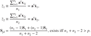
Since the goal is to find that ![]() which maximizes the distance between the group means, the problem is to maximize the squared distance:
which maximizes the distance between the group means, the problem is to maximize the squared distance:
The maximum of the squared distance occurs at ![]() given by
given by
An illustration of the discriminant analysis steps is done through the next example.
The use of the discriminant function for classification is considered next.
15.2.2 Classification
Let ![]() be a new vector of observation. The goal is to classify it into one of the groups by using the discriminant function. The simple, and fairly obvious, technique is to first obtain the discriminant score by
be a new vector of observation. The goal is to classify it into one of the groups by using the discriminant function. The simple, and fairly obvious, technique is to first obtain the discriminant score by
Next, classify ![]() to group 1 or 2 accordingly, as
to group 1 or 2 accordingly, as ![]() is closer to
is closer to ![]() or
or ![]() . A simple illustration is done next.
. A simple illustration is done next.
The function lda from the MASS package handles the Linear Discriminant Analysis very well. The particular reason for not using the function here is that our focus has been elucidation of the formulas in the scheme of flow of the theory. The results arising as a consequence of using the lda function by the command lda(GROUP˜X1+X2, data=rencher) is a bit different and the reader is asked to figure out the same. It goes without an explicit mention that the reader has a host of other options using the lda function.
15.3 Canonical Correlations
In multivariate data, we may have the case that there are two distinct subsets of vectors, with each subset characterizing certain traits of the unit of measurement. As an example, the marks obtained by a student in the examination for different subjects is one subset of measurements, whereas the performance in different sports may form another subset of measurements. Canonical correlations help us to understand the relationship between such sets of vector data.
Let ![]() and
and ![]() be two set of vectors measured on the same experimental unit. The goal of a canonical correlation study is to obtain vectors
be two set of vectors measured on the same experimental unit. The goal of a canonical correlation study is to obtain vectors ![]() and
and ![]() such that correlation between
such that correlation between ![]() and
and ![]() is a maximum, that is,
is a maximum, that is, ![]() is a maximum.
is a maximum.
The sample covariance matrix for the vector ![]() is
is
where ![]() is the sample covariance matrix of
is the sample covariance matrix of ![]() ,
, ![]() is the sample covariance matrix between
is the sample covariance matrix between ![]() and
and ![]() , and
, and ![]() of
of ![]() . A measure of association between the
. A measure of association between the ![]() ′s and the
′s and the ![]() ′s is given by
′s is given by
where ![]() , and
, and ![]() are the eigenvalues of
are the eigenvalues of ![]() . Note that the association measure
. Note that the association measure ![]() will be a poor measure, since each of the
will be a poor measure, since each of the ![]() values is between 0 and 1, and hence the product of such numbers approach 0 faster. However, the eigenvalues provide a useful measure of association between the vectors. Particularly, the square root of the eigenvalues leads to useful interpretations of the measures of the association. The collection of the square root of the eigenvalues
values is between 0 and 1, and hence the product of such numbers approach 0 faster. However, the eigenvalues provide a useful measure of association between the vectors. Particularly, the square root of the eigenvalues leads to useful interpretations of the measures of the association. The collection of the square root of the eigenvalues ![]() has been named the canonical correlations in the multivariate literature. Without loss of generality we assume that
has been named the canonical correlations in the multivariate literature. Without loss of generality we assume that ![]() .
.
As mentioned in Rencher (2002), the best overall measure of association between the ![]() ′s and
′s and ![]() ′s is the largest squared canonical correlation
′s is the largest squared canonical correlation ![]() . However, the other eigenvalues
. However, the other eigenvalues ![]() leading to the squared canonical correlations
leading to the squared canonical correlations ![]() also provide measures of supplemental dimensions of linear relationships between the
also provide measures of supplemental dimensions of linear relationships between the ![]() ′s and
′s and ![]() ′s.
′s.
The two important properties of canonical correlations as listed by Rencher are the following:
- Canonical correlations are scale invariant, scales of the
 ′s as well as the
  ′s.
′s. - The first canonical correlation
 is the maximum correlation among all linear combinations between the
  ′s and the
  ′s.
′s.
See Chapter 11 of Rencher for a comprehensive coverage of canonical correlations. We can test the independence of the ![]() ′s and the
′s and the ![]() ′s using any of the four tests discussed in Section 14.6. The concepts are illustrated for the Chemical Dataset of Box and Youle (1955) and are illustrated in Rencher.
′s using any of the four tests discussed in Section 14.6. The concepts are illustrated for the Chemical Dataset of Box and Youle (1955) and are illustrated in Rencher.
The next section is a very important concept in multivariate analysis.
15.4 Principal Component Analysis – Theory and Illustration
Principal Component Analysis (PCA) is a powerful data reduction tool. In the earlier multivariate studies we had ![]() components for a random vector. PCA considers the problem of identifying a new set of variables which explain more variance in the dataset. Jolliffe (2002) explains the importance of PCA as “The central idea of principal component analysis (PCA) is to reduce the dimensionality of a dataset consisting of a large number of interrelated variables, while retaining as much as possible of the variation present in the dataset.” In general, most of the ideas in multivariate statistics are extensions of the concepts from univariate statistics. PCA is an exception!
components for a random vector. PCA considers the problem of identifying a new set of variables which explain more variance in the dataset. Jolliffe (2002) explains the importance of PCA as “The central idea of principal component analysis (PCA) is to reduce the dimensionality of a dataset consisting of a large number of interrelated variables, while retaining as much as possible of the variation present in the dataset.” In general, most of the ideas in multivariate statistics are extensions of the concepts from univariate statistics. PCA is an exception!
Jolliffe (2002) considers the PCA theory and applications in a monumental way. Jackson (1991) is a very elegant exposition of PCA applications. For useful applications of PCA in chemometrics, refer to Varmuza and Filzmoser (2009). The development of this section is owed in a large extent to Jolliffe (2002) and Rencher (2002).
PCA may be useful in the following two cases: (i) too many explanatory variables relative to the number of observations; and (ii) the explanatory variables are highly correlated. Let us begin with a brief discussion of the math behind PCA.
15.4.1 The Theory
We begin with a discussion of population principal components. Consider a ![]() -variate normal random vector
-variate normal random vector ![]() with mean
with mean ![]() and variance-covariance matrix
and variance-covariance matrix ![]() . We assume that we have a random sample of
. We assume that we have a random sample of ![]() observations. The goal of PCA is to return a new set of variables
observations. The goal of PCA is to return a new set of variables ![]() , where each
, where each ![]() is some linear combination of the
is some linear combination of the ![]() s. Furthermore, and importantly, the
s. Furthermore, and importantly, the ![]() 's are in decreasing order of importance in the sense that
's are in decreasing order of importance in the sense that ![]() has more information about
has more information about ![]() 's than
's than ![]() , whenever
, whenever ![]() . The
. The ![]() 's are constructed in such a way that they are uncorrelated. Information here is used to convey the fact that the
's are constructed in such a way that they are uncorrelated. Information here is used to convey the fact that the ![]() whenever
whenever ![]() .
.
From its definition, the PCAs are linear combinations of the ![]() 's. The
's. The ![]() principal component is defined by
principal component is defined by
We know from the linearity of variance that we can specify the ![]() in such a way that variance of
in such a way that variance of ![]() can be infinite. Thus we may end up with components such that variance is infinite for each of them, which is of course meaningless. We will thus impose a restriction:
can be infinite. Thus we may end up with components such that variance is infinite for each of them, which is of course meaningless. We will thus impose a restriction:
We need to find ![]() such that
such that ![]() is a maximum. Next, we need to obtain
is a maximum. Next, we need to obtain ![]() such that
such that
and in general
For the first component, mathematically, we need to solve the maximization problem
where ![]() is a Lagrangian multiplier. As with an optimization problem, we will differentiate the above expression and equate the result to 0 for obtaining the optimal value of
is a Lagrangian multiplier. As with an optimization problem, we will differentiate the above expression and equate the result to 0 for obtaining the optimal value of ![]() :
:
Thus, we see that ![]() is an eigenvalue of
is an eigenvalue of ![]() and
and ![]() is the corresponding eigenvector. Since we need to maximize
is the corresponding eigenvector. Since we need to maximize ![]() , we select the maximum of the eigenvalue and its corresponding eigenvector for
, we select the maximum of the eigenvalue and its corresponding eigenvector for ![]() .
.
Let ![]() denote the
denote the ![]() eigenvalues of
eigenvalues of ![]() . We assume that the eigenvalues are distinct. Without loss of generality, we further assume that
. We assume that the eigenvalues are distinct. Without loss of generality, we further assume that ![]() . For the first PC we select the eigenvector corresponding to
. For the first PC we select the eigenvector corresponding to ![]() , that is,
, that is, ![]() is the eigenvector related to
is the eigenvector related to ![]() .
.
The second PC ![]() needs to maximize
needs to maximize ![]() and with the restriction that
and with the restriction that ![]() . Note that, post a few matrix computational steps,
. Note that, post a few matrix computational steps,
Thus, the constraint that the first two PCs are uncorrelated may be specified by ![]() . The maximization problem for the second PC is specified in the equation below:
. The maximization problem for the second PC is specified in the equation below:
where ![]() are the Lagrangian multipliers. We need to optimize the above equation and obtain the second PC. As we generally do with optimization problems, we will differentiate the maximization statement with respect to
are the Lagrangian multipliers. We need to optimize the above equation and obtain the second PC. As we generally do with optimization problems, we will differentiate the maximization statement with respect to ![]() and obtain:
and obtain:
which by multiplication of the left-hand side by ![]() gives us
gives us
Since ![]() , the first two terms of the above equation equal zero and since
, the first two terms of the above equation equal zero and since ![]() , we get
, we get ![]() . Substituting this into the two displayed expressions above, we get
. Substituting this into the two displayed expressions above, we get ![]() . On readjustment, we get
. On readjustment, we get ![]() , and we again see
, and we again see ![]() as the eigenvalue of
as the eigenvalue of ![]() . Under the assumption of distinct eigenvalues for
. Under the assumption of distinct eigenvalues for ![]() , we choose the second largest eigenvalue and its corresponding eigenvector for
, we choose the second largest eigenvalue and its corresponding eigenvector for ![]() . We proceed in a similar way for the rest of the
. We proceed in a similar way for the rest of the ![]() PCs. As with the first PC,
PCs. As with the first PC, ![]() is chosen as the eigenvector corresponding to
is chosen as the eigenvector corresponding to ![]() for
for ![]() .
.
The variance of the ![]() principal component
principal component ![]() is
is
The amount of variation explained by the ![]() PC is
PC is
Since the PCs are uncorrelated, the variation explained by the first ![]() PCs is
PCs is

The variance explained by the PCs are best understood through a screeplot. A screeplot looks like the profile of a mountain where after a steep slope a flatter region appears that is built by fallen and deposited stones (called scree). Therefore, this plot is often named as the SCREE PLOT. It is investigated from the top until the debris is reached. This explanation is from Varmura and Filzmoser (2009).
The development thus far focuses on population principal components, which involve unknown parameters ![]() and
and ![]() . Since these parameters are seldom known, the sample principal components are obtained by replacing the unknown parameters with their respective MLEs. If the observations are on different scales of measurements, a practical rule is to use the sample correlation matrix instead of the covariance matrix.
. Since these parameters are seldom known, the sample principal components are obtained by replacing the unknown parameters with their respective MLEs. If the observations are on different scales of measurements, a practical rule is to use the sample correlation matrix instead of the covariance matrix.
The covariance between observation ![]() and PC
and PC ![]() is given by
is given by
and the correlation is

However, if the PCs are extracted from the correlation matrix, then
The concepts will be demonstrated in the next subsection.
15.4.2 Illustration Through a Dataset
We will use two datasets for the usage of PCA.
In the next subsection, we focus on the applications of PCA.
15.5 Applications of Principal Component Analysis
Jolliffe (2002) and Jackson (1991) are two detailed treatises which discuss variants of PCA and their applications. PCA can be applied and/or augmented by statistical techniques such as ANOVA, linear regression, Multidimensional scaling, factor analysis, microarray modeling, time series, etc.
15.5.1 PCA for Linear Regression
Section 12.6 indicated the problem of multicollinearity in linear models. If the covariates are replaced with the PCs, the problem of multicollinearity will cease, since the PCs are uncorrelated with each other. It is thus the right time to fuse the multicollinearity problems of linear models with PCA. We are familiar with all the relevant concepts and hence will take the example of Maindonald and Braun (2009) for throwing light on this technique. Maindonald and Braun (2009) have made the required dataset available in their package DAAG. See Streiner and Norman (2003) for more details of this study.
It is thus seen how the PCA helps to reduce the number of variables in the linear regression model. Note that even if we replace the original variables with equivalent PCs, the problem of multicollinearity is fixed.
15.5.2 Biplots
Gower and Hand (1996) have written a monograph on the use of biplots for multivariate data. Gower, et al. (2011) is a recent book on biplots complemented with the R package UBbipl, and is also an extension of Gower and Hand (1996). Greenacre (2010) has implemented all the biplot techniques in his book. This book has R codes for doing all the data analysis, and he has also been very generous to gift it to the world at http://www.multivariatestatistics.org/biplots.html. For theoretical aspects of biplots, the reader may also refer to Rencher (2002), Johnson and Wichern (2007), and Jolliffe (2002) among others. For a simpler and effective understanding of the biplots, see the Appendix of Desmukh and Purohit (2007).
The biplot is a visualization technique of the data matrix ![]() through two coordinate systems representing the observations (row) and variables (columns) of the dataset. In this method, the variance-covariance between the variable and the distance between the observations, are plotted in a single figure, and to reflect this facet the prefix “bi” is used here. In this plot, the distance between the points, which are observations, represents the Mahalanobis distance between them. The length of a vector, displayed on the plot, from the origin to the coordinates, represents the variance of the variable with the angle between the variables (represented by the vectors) denoting the correlation. If the angle between the vectors is small, it will indicate that the vectors are strongly correlated.
through two coordinate systems representing the observations (row) and variables (columns) of the dataset. In this method, the variance-covariance between the variable and the distance between the observations, are plotted in a single figure, and to reflect this facet the prefix “bi” is used here. In this plot, the distance between the points, which are observations, represents the Mahalanobis distance between them. The length of a vector, displayed on the plot, from the origin to the coordinates, represents the variance of the variable with the angle between the variables (represented by the vectors) denoting the correlation. If the angle between the vectors is small, it will indicate that the vectors are strongly correlated.
For the sake of simplicity, we will assume that the data matrix ![]() , consisting of
, consisting of ![]() observations of a
observations of a ![]() -dimensional vector, is a centered matrix in the sense that each column has a zero mean. By the singular value decomposition, SVD, result, we can write the matrix
-dimensional vector, is a centered matrix in the sense that each column has a zero mean. By the singular value decomposition, SVD, result, we can write the matrix ![]() as
as
where ![]() is an
is an ![]() matrix,
matrix, ![]() is an diagonal
is an diagonal ![]() matrix, and
matrix, and ![]() is an
is an ![]() matrix. By the properties of SVD, we have
matrix. By the properties of SVD, we have ![]() and
and ![]() . Furthermore,
. Furthermore, ![]() has diagonal elements in
has diagonal elements in ![]() . We will consider a simple illustration of the SVD for the famous “Cork” dataset of Rao (1973).
. We will consider a simple illustration of the SVD for the famous “Cork” dataset of Rao (1973).
Notice the decline of the singular values, ![]() values, for the cork dataset. In the spirit of PCA, we tend to believe that if such a decline is steep, we can probably have a good understanding of the dataset if we resort to some plots which use two variables. In fact, such a result is validated by a theorem of Eckart and Young (1936). We need to connect the SVD result with the well-known quadratic decomposition, QR, result, which is now stated. The QR decomposition says that any
values, for the cork dataset. In the spirit of PCA, we tend to believe that if such a decline is steep, we can probably have a good understanding of the dataset if we resort to some plots which use two variables. In fact, such a result is validated by a theorem of Eckart and Young (1936). We need to connect the SVD result with the well-known quadratic decomposition, QR, result, which is now stated. The QR decomposition says that any ![]() matrix can be expressed as
matrix can be expressed as
where ![]() is an
is an ![]() matrix and
matrix and ![]() is an
is an ![]() matrix, and
matrix, and ![]() is the rank of matrix
is the rank of matrix ![]() . In a certain sense, the goal is to understand the variance among the
. In a certain sense, the goal is to understand the variance among the ![]() observations through the matrix
observations through the matrix ![]() and the variance among the
and the variance among the ![]() variables through
variables through ![]() . The matrices
. The matrices ![]() and
and ![]() may be obtained as a combination of the SVD elements as
may be obtained as a combination of the SVD elements as ![]() and
and ![]() . For different choices of
. For different choices of ![]() , we have different representations for
, we have different representations for ![]() . The three most common choices of
. The three most common choices of ![]() are 0, 1/2, and 1, see Gabriel (1971). We mention some consequences of these choices, see Khatree and Naik (1999).
are 0, 1/2, and 1, see Gabriel (1971). We mention some consequences of these choices, see Khatree and Naik (1999).
 . In the this case, the QR matrices may be expressed in terms of the SVD matrices as
15.15
. In the this case, the QR matrices may be expressed in terms of the SVD matrices as
15.15
For the choice
 , we place an equal emphasis on the variables and the observations.
 . Here15.16
The distance between the vectors
 approximates the squared Mahalanobis distance between the observation vectors. Furthermore, the inner product between the vectors
  approximates the covariances between them and length of a vector
  gives its variance.
 . Here,15.17
For this case, the distance between
 's is the usual Euclidean distance between them and the values of
  equals the principal component score for the observations, whereas the values of
  refer to the principal component loadings.
For the cork dataset, we will obtain the biplot for the choice ![]() .
.
15.6 Factor Analysis
We will have a look at another important facet of multivariate statistical analysis: Factor Analysis. The data observations ![]() , are assumed to arise from an
, are assumed to arise from an ![]() distribution. Consider a hypothetical example where the correlation matrix is given by
distribution. Consider a hypothetical example where the correlation matrix is given by

Here, we can see that the first two components are strongly correlated with each other and also appear to be independent of the rest of the components. Similarly, the last three components are strongly correlated among themselves and independent of the first two components. A natural intuition is to think of the first two components arising due to one factor and the remaining three due to a second factor. The factors are also sometimes called latent variables.
The development in the rest of the section is only related to orthogonal factor model and it is the same whenever we talk about the factor analysis model. For other variants, refer to Basilevsky (1994), Reyment and J'oreskog (1996), and Brown (2006).
15.6.1 The Orthogonal Factor Analysis Model
Let ![]() be a
be a ![]() -vector. To begin with, we will assume that there are
-vector. To begin with, we will assume that there are ![]() factors with
factors with ![]() and that each of the
and that each of the ![]() 's is a function of the
's is a function of the ![]() factors. The factor analysis model is given by
factors. The factor analysis model is given by
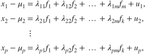
where ![]() , are normally distributed errors associated with the variable
, are normally distributed errors associated with the variable ![]() . In the factor analysis model, the
. In the factor analysis model, the ![]() , are the regression coefficients between the observed variables and the factors. Two points need to be observed. In the factor analysis literature, the regression coefficients are called loadings, which indicate how the weights of the
, are the regression coefficients between the observed variables and the factors. Two points need to be observed. In the factor analysis literature, the regression coefficients are called loadings, which indicate how the weights of the ![]() 's depend on the factors
's depend on the factors ![]() 's. The loadings are denoted by
's. The loadings are denoted by ![]() 's, which we thus far used for eigenvalues and eigenvectors. However, the notation of
's, which we thus far used for eigenvalues and eigenvectors. However, the notation of ![]() 's for the loadings is standard in the factor analysis literature and in the rest of this section they will denote the loadings and not quantities related to eigenvalues.
's for the loadings is standard in the factor analysis literature and in the rest of this section they will denote the loadings and not quantities related to eigenvalues.
We will now use the matrix notation and then state the essential assumptions. The (orthogonal) factor model may be stated in matrix form as
where
The essential assumptions related to the factors are as follows:
Under the above assumptions, we can see that the variance of component ![]() can be expressed in terms of the loadings as
can be expressed in terms of the loadings as

Define ![]() . Thus, the variance of a component can be written as the sum of a common variance component and a specific variance component. It is common practice in the factor analysis literature to refer to
. Thus, the variance of a component can be written as the sum of a common variance component and a specific variance component. It is common practice in the factor analysis literature to refer to ![]() as the common variance and the specific variance
as the common variance and the specific variance ![]() as specificity, unique variance, or residual variance.
as specificity, unique variance, or residual variance.
The covariance matrix ![]() can be written in terms of
can be written in terms of ![]() and
and ![]() as
as
Using the above relationship, we can arrive at the next expression:
We will consider three methods for estimation of the loadings and communalities: (i) The Principal Component Method, (ii) The Principal Factor Method, and (iii) Maximum Likelihood Function. We omit a fourth important technique of estimation of factors in “Iterated Principal Factor Method”.
15.6.2 Estimation of Loadings and Communalities
We will first consider the principal component method. Let ![]() denote the sample covariance matrix. The problem is then to find an estimator
denote the sample covariance matrix. The problem is then to find an estimator ![]() , which will approximate
, which will approximate ![]() such that
such that
In this approach, the last component ![]() is ignored and we approximate the sampling covariance matrix by a spectral decomposition:
is ignored and we approximate the sampling covariance matrix by a spectral decomposition:
where ![]() is an orthogonal matrix constructed with normalized eigenvectors,
is an orthogonal matrix constructed with normalized eigenvectors, ![]() , of
, of ![]() and
and ![]() is a diagonal matrix with eigenvalues of
is a diagonal matrix with eigenvalues of ![]() . That is, if
. That is, if ![]() are the eigenvalues of
are the eigenvalues of ![]() , then
, then ![]() . Since the eigenvalues
. Since the eigenvalues ![]() of the positive semi-definite matrix
of the positive semi-definite matrix ![]() are all positive or zero, we can factor
are all positive or zero, we can factor ![]() as
as
and substituting this in (15.28), we get

This suggests that we can use ![]() . However, we seek a
. However, we seek a ![]() whose order is less than
whose order is less than ![]() , and hence we consider the first
, and hence we consider the first ![]() largest
largest ![]() eigenvalues and take
eigenvalues and take ![]() and
and ![]() with their corresponding eigenvectors. Thus, an useful estimator of
with their corresponding eigenvectors. Thus, an useful estimator of ![]() is given by
is given by
Note that the ![]() diagonal element of
diagonal element of ![]() is the sum of squares of
is the sum of squares of ![]() . We can then use this to estimate the diagonal elements of
. We can then use this to estimate the diagonal elements of ![]() by
by
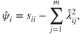
and using this relationship approximate ![]() by
by
Since, here, the sums of squares of the rows and columns of ![]() equal the communalities and eigenvalues respectively, an estimate of the
equal the communalities and eigenvalues respectively, an estimate of the ![]() communality is given by
communality is given by

Similarly, we have
where the last equality follows from the fact that ![]() . Using the estimates of
. Using the estimates of ![]() and
and ![]() in (15.29), we obtain a partition of the variance of the
in (15.29), we obtain a partition of the variance of the ![]() variable as
variable as
The contribution of the ![]() factor to the total sample variance is therefore
factor to the total sample variance is therefore
We will now illustrate the concepts with a solved example from Rencher (2002).
We will next consider the principal factor method. In the previous method we have omitted ![]() . In the principal factor method we use an initial estimate of
. In the principal factor method we use an initial estimate of ![]() , say
, say ![]() , and factor for
, and factor for ![]() , or
, or ![]() , whichever is appropriate:
, whichever is appropriate:
where ![]() is as specified in (15.30) with the eigenvalues and eigenvectors of
is as specified in (15.30) with the eigenvalues and eigenvectors of ![]() or
or ![]() . Since the
. Since the ![]() diagonal element of
diagonal element of ![]() is the
is the ![]() communality, we have
communality, we have ![]() . In the case of
. In the case of ![]() , we have
, we have ![]() . For more details, refer to Section 13.2 of Rencher (2002). We will illustrate these computations as a continuation of the previous example.
. For more details, refer to Section 13.2 of Rencher (2002). We will illustrate these computations as a continuation of the previous example.
Finally, we conclude this section with a discussion of the Maximum Likelihood Estimation method. Under the assumption that the observations ![]() are a random sample from
are a random sample from ![]() , it may be shown that the estimates
, it may be shown that the estimates ![]() and
and ![]() satisfy the following set of equations:
satisfy the following set of equations:
The equations need to be solved iteratively, and happily for us R does that. The MLE technique is illustrated in the next example. We need to address a few important questions before then.
The important question is regarding the choice of the number of factors to be determined. Some rules given in Rencher are stated in the following.
- Select
 as equal to the number of factors necessary, which account for a pre-specified percentage of the variance accounted by the factors, say 80%.
 - Select
 as the number of eigenvalues that are greater than the average eigenvalue.
 - Use a screeplot to determine
 .
. - Test the hypothesis that
 is the correct number of factors, that is,
 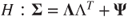 .
.
We leave it to the reader to find out more about the concept of Rotation and give a summary of them, adapted from Hair, et al. (2010).
- Varimax Rotation is the most popular orthogonal factor rotation method, which focuses on simplifying the columns of a factor matrix. It is generally superior to other orthogonal factor rotation methods. Here, we seek to rotate the loadings, which maximize the variance of the squared loadings in each column of
 .
. - Quartimax Rotation is a less powerful technique than varimax rotation, which focuses on simplifying the columns of the factor matrix.
- Oblique Rotation obtains the factors such that the extracted factors are correlated, and hence it identifies the extent to which the factors are correlated.
We have thus learnt about fairly complex and powerful techniques in multivariate statistics. The techniques vary from classifying observations to specific class, identifying group of independent (sub) vectors, reducing the number of variables, and determining hidden variables which possibly explain the observed variables. More details can be found in the references concluding this chapter.
15.7 Further Reading
We will begin with a disclaimer that the classification of the texts in different sections is not perfect.
15.7.1 The Classics and Applied Perspectives
Anderson (1958, 1984, and 2003) are the first primers on MSA. Currently, Anderson's book is in its third edition and it is worth noting that the second and third editions are probably the only ones which discuss the Stein effect in depth. Chapter 8 of Rao (1973) provides the necessary theoretical background for multivariate analysis and also contains some of Rao's remarkable research in multivariate statistics. In a certain way, one chapter may have more results than we can possibly cover in a complete book. A vector space approach for multivariate statistics is to be found in Eaton (1983, 2007). Mardia, Kent, and Bibby (1979) is an excellent treatise on multivariate analysis and considers many geometrical aspects. The geometrical approach is also considered in Gnanadesikan (1977, 1997), and further robustness aspects are also developed within it. Muirhead (1982), Giri (2004), Bilodeau and Brenner (1999), Rencher (2002), and Rencher (1998) are among some of the important texts on multivariate analysis. We note here that our coverage is mainly based on Rencher (2002).
Jolliffe (2002) is a detailed monograph on Principal Component Analysis. Jackson (1991) is a remarkable account on the applications on PCA. It is needless to say that if you read through these two books, you may become an authority on PCA.
Missing data, EM algorithms, and multivariate analysis have been aptly handled in Schafer (1997) and in fact many useful programs have been provided in S, which can be easily adapted in R. In this sense, this is a stand-alone reference book which deals with missing data. Of course, McLachlan and Krishnan (2008) may also be used!
Johnson and Wichern (2007) is a popular course, which does apt justice between theory and applications. Hair, et al. (2010) may be commonly found on a practitioner's desk. Izenman (2008) is a modern flavor of multivariate statistics with converage of the fashionable area of machine learning. Sharma (1996) and Timm (2002) also provide a firm footing in multivariate statistics.
Gower, et al. (2011) discuss many variants of biplots, which is an extension of Gower and Hand (1996). Greenacre (2010) is an open source book with in-depth coverage of biplots.
15.7.2 Multivariate Analysis and Software
The two companion volumes of Khatree and Naik (1999) and Khatree and Naik (2000) provide excellent coverage of multivariate analysis and computations through SAS software. It may be noted, one more time, that the programs and logical thinking are of paramount importance rather than a particular software. It is worth recording here that these two companions provide a fine balance between the theoretical aspects and computations. H'ardle and Simar (2007) have used “XploRe” software for computations. Last, and not least, the most recent book of Everitt and Hothorn (2011) is a good source for multivariate analysis through R. Varmuza and Filzmoser (2009) have used R software with a special emphasis on the applications to Chemometrics. Husson, et al. (2011) is also a recent arrival, which integrates R with multivariate analysis. Desmukh and Purohit (2007) also present PCA, biplot, and other multivariate aspects in R, though their emphasis is more on microarray data.
15.8 Complements, Problems, and Programs
Problem 15.1 Explore the R examples for linear discriminant analysis and canonical correlation with
example(lda)andexample(cancor).Problem 15.2 In the “Seishu Wine Study” of Example 16.9.1, the tests for independence of four sub-vectors lead to rejection of the hypothesis of their independence. Combine the subvectors
s11withs22ands33withs44. Find the canonical correlations between these combined subvectors. Furthermore, find the canonical correlations for each subvector while pooling the others together.Problem 15.3 Principal components offer effective reduction in data dimensionality. In Examples 15.4.1 and 15.4.2, it is observed that the first few PCs explain most of the variation in the original data. Do you expect further reduction if you perform PCA on these PCs? Validate your answer by running
princompon the PCs.Problem 15.4 Find the PCs for the stack loss dataset, which explain 85% of the variation in the original dataset.
Problem 15.5 Perform the PCA on the
irisdataset along the two lines: (i) the entire dataset, (ii) three subsets according to the three species. Check whether the PC scores are significantly different across the three species using an appropriate multivariate testing problem.Problem 15.6 For the US crime data of Example 13.4.2, carry out the PCA for the covariates and then perform the regression analysis on the PC scores. Investigate if the multicollinearity problem persists in the fitted regression model based on the PC scores.
Problem 15.7 How do outliers effect PC scores? Perform PCA on the board stiffness dataset of Example 16.3.5 with and without the detected outliers therein.
Problem 15.8 Check out for the example of the
factanalfunction. Are factors present in theirisdataset? Develop the complete analysis for the problem.