Chapter 10
Stochastic Processes
Package(s): sna
Dataset(s): testtpm, testtpm2, testtpm3
10.1 Introduction
Stochastic processes commonly refer to a collection of random variables. Such a collection may vary over time, sample number, geographical location, etc. It is to be noted that a stochastic process may consist of finite, countably infinite, or uncountably infinite collections of random variables. An important characteristic of the stochastic process is that it allows us to relax the assumption of independence for a sequence of random variables.
A few examples are in order.
Section 10.2 will ensure that the probability space for the stochastic process is properly defined. A very important class of stochastic process is the Markov Chains, and this will be detailed in Section 10.3. The chapter will close with a brief discussion of how Markov Chains are useful in the practical area of computational statistics in Section 10.4.
10.2 Kolmogorov's Consistency Theorem
As seen in the introductory section, a stochastic process is a collection of infinite random variables. It needs to be ensured that the probability measures are well defined for such a collection of RVs. An affirmative answer in this direction is provided by Prof Kolmogorov. The related definitions and theorems (without proof) have been adapted from Adke and Manjunath (1984) and Athreya and Lahiri (2005). We consider the probability space ![]() and follow it up with a sequence of RVs
and follow it up with a sequence of RVs ![]() . Here
. Here ![]() is any non-empty set. Then for any
is any non-empty set. Then for any ![]() , the random vector
, the random vector ![]() has a joint probability distribution
has a joint probability distribution ![]() over
over ![]() , and here
, and here ![]() is the Borel
is the Borel ![]() -field over
-field over ![]() .
.
For any ![]() , and any
, and any ![]() , the family of fdds satisfies the following two conditions:
, the family of fdds satisfies the following two conditions:
- [C1].
10.3

- [C2]. For any permutation
 of
of  :
10.4
:
10.4
Kolmogorov's consistency theorem addresses the issue that if there exists a family of distributions ![]() in finite dimensional Euclidean spaces, then there exists a real valued stochastic process
in finite dimensional Euclidean spaces, then there exists a real valued stochastic process ![]() whose fdds coincides with
whose fdds coincides with ![]() .
.
Having being assured of the existence of probability measures for the stochastic processes, let us now look at the important family of stochastic processes: Markov Chains.
10.3 Markov Chains
In earlier chapters, we assumed the observations were independent. In many random phenomenon, the observations are not independent. As seen in the examples in Section 10.1, the maximum temperature of the current day may depend on the maximum temperature of the previous day. The sum of heads in ![]() trials depends on the corresponding sum in the first
trials depends on the corresponding sum in the first ![]() trials. Markov Chains are useful for tackling such dependent observations. In this section, we will be considering only discrete phenomenon.
trials. Markov Chains are useful for tackling such dependent observations. In this section, we will be considering only discrete phenomenon.
To begin with, we need to define the state space associated with the sequence of random variables. The state space is the set of possible values taken by the stochastic process. In Example 10.1.1 of Section 10.1, the state space for the sum of heads in ![]() throws of a coin is
throws of a coin is ![]() . The state space considered in this section is at most countably infinite. At time
. The state space considered in this section is at most countably infinite. At time ![]() , the stochastic process
, the stochastic process ![]() will take one of the values in
will take one of the values in ![]() , that is,
, that is, ![]() .
.
This definition says that the probability of ![]() being observed in a state
being observed in a state ![]() , given the entire history
, given the entire history ![]() , depends only on the recent past state of
, depends only on the recent past state of ![]() , and not on the history. The matrix array
, and not on the history. The matrix array ![]() is called the Transition Probability Matrix, abbreviated as TPM, of the Markov Chain.
is called the Transition Probability Matrix, abbreviated as TPM, of the Markov Chain.
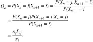
In the next subsection, we will consider how the states of a Markov Chain can be classified into a meaningful set of various characteristics.
10.3.1 The m-Step TPM
The TPM ![]() is a one-step transition probability array, namely, its elements give the probability of moving from state
is a one-step transition probability array, namely, its elements give the probability of moving from state ![]() to state
to state ![]() in the next step. The
in the next step. The ![]() -step transition probability of a movement from state
-step transition probability of a movement from state ![]() to state
to state ![]() is defined by
is defined by
Let ![]() denote the
denote the ![]() -step transition probability matrix. It can be shown that
-step transition probability matrix. It can be shown that
Equation 10.8 is based on the well-known Chapman-Kolmogorov equation. The Chapman-Kolmogorov lemma says that for any ![]()
We can easily use the Chapman-Kolmogorov relationship to obtain the ![]() -step TPM of a Markov Chain. The R program for obtaining the
-step TPM of a Markov Chain. The R program for obtaining the ![]() -step TPM through
-step TPM through msteptpm is given in the next illustration.
10.3.2 Classification of States
In the Ehrenfest example we see that it is possible to move from a particlar state to one of its adjacent states only. However, it is possible for us to move from state 1 to states 3 and 4 in 2 and 3 steps. The question that then arises is how to identify the accessible states? Towards this discussion, a few definitions are required.
Accessibility is denoted by ![]() .
.
Communication between two states is denoted by ![]() . The collection of the states where each communicates with the other is said to belong to the same class. Some properties of communication, without proof, are listed below:
. The collection of the states where each communicates with the other is said to belong to the same class. Some properties of communication, without proof, are listed below:
 .
.- If
 , then
  .
. - If
 and
and  , then
  .
.
Irreducible Markov Chains are also called ergodic Markov Chains. A stronger requirement than irreducibility is given next.
It can be easily seen that the presence of an absorbing state implies that the Markov Chain is neither regular nor irreducible.
A state ![]() is said to have period
is said to have period ![]() if
if ![]() whenever
whenever ![]() is not divisible by
is not divisible by ![]() and
and ![]() is the greatest integer with this property. The period of a state is denoted by
is the greatest integer with this property. The period of a state is denoted by ![]() . If it is not possible to return to state
. If it is not possible to return to state ![]() and be retained in
and be retained in ![]() (starting from state
(starting from state ![]() of course), the period of the state
of course), the period of the state ![]() is infinite. On the other hand, if a state has period 1, we call that state aperiodic.
is infinite. On the other hand, if a state has period 1, we call that state aperiodic.
Digraph is a powerful visualizing tool for understanding the accessible and communicating states of a Markov Chain. Here, we use the package sna for achieving this. Note that this package is developed for the purpose of an emerging field Social Network Analysis. The gplot function from this package is useful for our purpose though.
10.3.3 Canonical Decomposition of an Absorbing Markov Chain
In the previous discussion we have seen different types of TPM characteristics for the Markov Chains. In an irreducibile Markov Chain, all the states are recurrent states. However, if there is an absorbing state, as in testtpm, we may be interested in the following issues:
- 1. The probability of the process ending up in an absorbing state.
- 2. The average time for the Markov Chain to get absorbed.
- 3. The average time spent in each of the transient states.
The canonical decomposition helps with the answer to the above questions.
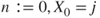
Arrange the states of an absorbing Markov Chain in the form of (TRANSIENT, ABSORBING). For example, reorder the states of testtpm2 as ![]() . Let
. Let ![]() be the number of absorbing states and
be the number of absorbing states and ![]() the number of transient states. The total number of states is
the number of transient states. The total number of states is ![]() . Arrange the TPM as below:
. Arrange the TPM as below:
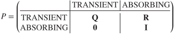
Here ![]() is an
is an ![]() identity matrix,
identity matrix, ![]() an
an ![]() zero matrix,
zero matrix, ![]() a
a ![]() matrix, and
matrix, and ![]() a non-zero
a non-zero ![]() matrix. Let us closely look at the matrix
matrix. Let us closely look at the matrix ![]() and calculate
and calculate ![]() for some large
for some large ![]() . Note that it is very easy to rearrange the matrix in the required form in R.
. Note that it is very easy to rearrange the matrix in the required form in R.
> testtpm <- as.matrix(testtpm)
> testtpm <- testtpm[c(2,3,4,5,1,6),c(2,3,4,5,1,6)]
> Q <- testtpm[c(1:4),c(1:4)]
> R <- testtpm[c(1:4),c(5,6)]
> Q
     B     C    D    E
B 0.50 0.000 0.25 0.00
C 0.00 0.000 1.00 0.00
D 0.25 0.125 0.25 0.25
E 0.00 0.000 0.25 0.50
> R
       A      F
B 0.2500 0.0000
C 0.0000 0.0000
D 0.0625 0.0625
E 0.0000 0.2500
> testtpm
     B     C    D    E      A      F
B 0.50 0.000 0.25 0.00 0.2500 0.0000
C 0.00 0.000 1.00 0.00 0.0000 0.0000
D 0.25 0.125 0.25 0.25 0.0625 0.0625
E 0.00 0.000 0.25 0.50 0.0000 0.2500
A 0.00 0.000 0.00 0.00 1.0000 0.0000
F 0.00 0.000 0.00 0.00 0.0000 1.0000
> msteptpm(testtpm,n=100)[c(1:4),c(1:4)]
             B            C            D            E
B 1.635836e-10 3.124169e-11 2.022004e-10 1.635836e-10
C 2.499335e-10 4.773305e-11 3.089348e-10 2.499335e-10
D 2.022004e-10 3.861685e-11 2.499335e-10 2.022004e-10
E 1.635836e-10 3.124169e-11 2.022004e-10 1.635836e-10
We can easily then see that
The Fundamental Matrix for an absorbing Markov chain is given by
The elements ![]() of
of ![]() gives the expected number of times the process will be in transient state
gives the expected number of times the process will be in transient state ![]() if the process started in state
if the process started in state ![]() . For the
. For the testtpm example, we have the answers in the output given below:
> N <- solve(diag(rep(1,nrow(Q)))-Q)
> N
          B         C        D         E
B 2.6666667 0.1666667 1.333333 0.6666667
C 1.3333333 1.3333333 2.666667 1.3333333
D 1.3333333 0.3333333 2.666667 1.3333333
E 0.6666667 0.1666667 1.333333 2.6666667
Starting from a transient state ![]() , the expected number of steps before the Markov Chain is absorbed and the probabilities of it being absorbed into one of the absorbing states are respectively given by
, the expected number of steps before the Markov Chain is absorbed and the probabilities of it being absorbed into one of the absorbing states are respectively given by
where ![]() is an
is an ![]() column of 1 and
column of 1 and ![]() and
and ![]() are respectively the expected number of steps and probabilities of the absorption matrix. For our dummy example, the computation concludes with the program below.
are respectively the expected number of steps and probabilities of the absorption matrix. For our dummy example, the computation concludes with the program below.
> t <- N
> t
      [,1]
B 4.833333
C 6.666667
D 5.666667
E 4.833333
> B <- N %*% R
> B
     A    F
B 0.75 0.25
C 0.50 0.50
D 0.50 0.50
E 0.25 0.75
The three questions asked about an absorbing Markov Chain are also applicable to an Ergodic Markov Chain in a slightly different sense. This topic will be taken up next.
10.3.4 Stationary Distribution and Mean First Passage Time of an Ergodic Markov Chain
If we have an ergodic Markov Chain, we know that each state will be visited infinitely often. However, this implies that over the long run, the number of times it will be in a given state may be obtained.
A stationary distribution ![]() is a (left) eigenvector of the TPM whose associated eigenvalue is equal to one. For an ergodic Markov Chain, the next program gives us the stationary distribution.
is a (left) eigenvector of the TPM whose associated eigenvalue is equal to one. For an ergodic Markov Chain, the next program gives us the stationary distribution.
> stationdistTPM <- function(M){
+       eigenprob <- eigen(t(M))
+       temp <- which(round(eigenprob$values,1)==1)
+       stationdist <- eigenprob$vectors[,temp]
+       stationdist <- stationdist/sum(stationdist)
+       return(stationdist)
+ }
> P <- matrix(nrow=3,ncol=3) # An example
> P[1,] <- c(1/3,1/3,1/3)
> P[2,] <- c(1/4,1/2,1/4)
> P[3,] <- c(1/6,1/3,1/2)
> stationdistTPM(P)
[1] 0.24 0.40 0.36
The function uses the eigen function to obtain the eigenvalues and eigenvectors.
The mean recurrence time of an ergodic Markov Chain is given by
For the previous example:
> 1/stationdistTPM(P)
[1] 4.166667 2.500000 2.777778
We will next consider the concept of passage time.
The matrix of mean first passage time is denoted by ![]() . We will next briefly state the formulas to obtain
. We will next briefly state the formulas to obtain ![]() . Let
. Let ![]() be a matrix where each row consists of the stationary probability vector. Define
be a matrix where each row consists of the stationary probability vector. Define ![]() , where
, where ![]() is an identity matrix, and
is an identity matrix, and ![]() is a matrix where each row is the stationary probability vector
is a matrix where each row is the stationary probability vector ![]() . The elements of
. The elements of ![]() are then given by
are then given by
For the Ehrenfest model, the mean recurrence times are given below:
> ehrenfest <- as.matrix(ehrenfest)
> w <- stationdistTPM(ehrenfest)
> W <- matrix(rep(w,each=nrow(ehrenfest)),nrow=nrow(ehrenfest))
> Z <- solve(diag(rep(1,nrow(ehrenfest)))-ehrenfest+W)
> M <- ehrenfest*0
> for(i in 1:nrow(ehrenfest)){
+     for(j in 1:nrow(ehrenfest)){
+ M[i,j] <- (Z[j,j]-Z[i,j])/W[j,j]
+ }
+ }
> M
         0        1        2        3        4
0  0.00000 1.000000 2.666667 6.333333 21.33333
1 15.00000 0.000000 1.666667 5.333333 20.33333
2 18.66667 3.666667 0.000000 3.666667 18.66667
3 20.33333 5.333333 1.666667 0.000000 15.00000
4 21.33333 6.333333 2.666667 1.000000  0.00000
For details, refer to Chapter 11 of Grinstead and Snell (2002).
10.3.5 Time Reversible Markov Chain
Consider a stationary and ergodic Markov Chain with stationary distribution ![]() .
.
In simple words, for a stationary ergodic Markov Chain with ![]() , the backward chain
, the backward chain ![]() is also a Markov Chain. An intuitive explanation of the phenomenon is that given the present state, the past and future states are independent events. The TPM of the reversed Markov Chain is given by
is also a Markov Chain. An intuitive explanation of the phenomenon is that given the present state, the past and future states are independent events. The TPM of the reversed Markov Chain is given by ![]() :
:
The Gamblers random walk in a finite state space is an example of time reversible Markov Chain.
10.4 Application of Markov Chains in Computational Statistics
Modern computations are driven by hi-speed computers and without the latter some of the algorithms cannot be put to good use. In this section two of the famous Monte Carlo techniques will be discussed whose premise is in the usage of Markov Chains, viz., the Metropolis-Hastings algorithm and the Gibbs sampler. The current section relies on Chapter 10 of Ross (2006).1 Robert and Casella (1999–2004) is also an excellent exposition for the two algorithms to be discussed here.
10.4.1 The Metropolis-Hastings Algorithm
Consider a finite sequence of positive numbers ![]() , for some large integer
, for some large integer ![]() . The positive numbers may be interpreted as the weights of an RV
. The positive numbers may be interpreted as the weights of an RV ![]() taking the values
taking the values ![]() . Define
. Define ![]() , and suppose that
, and suppose that ![]() is a difficult number to compute. The PMF of
is a difficult number to compute. The PMF of ![]() is then given by
is then given by

It will be seen in Chapter 11 that for large ![]() values, simulation from the probability distribution
values, simulation from the probability distribution ![]() becomes a daunting task. The Metropolis-Hastings algorithm builds a time-reversible Markov Chain argument for simulation from
becomes a daunting task. The Metropolis-Hastings algorithm builds a time-reversible Markov Chain argument for simulation from ![]() . The requirement is then to find a Markov Chain with TPM
. The requirement is then to find a Markov Chain with TPM ![]() , which is easier to simulate and its stationary distribution must be the same as
, which is easier to simulate and its stationary distribution must be the same as ![]() . Let
. Let ![]() represent the TPM of an irreducible time-reversible Markov Chain. A Markov Chain
represent the TPM of an irreducible time-reversible Markov Chain. A Markov Chain ![]() , useful for simulation from
, useful for simulation from ![]() , is set up as follows. Suppose that the current state is
, is set up as follows. Suppose that the current state is ![]() , that is,
, that is, ![]() . Generate an RV
. Generate an RV ![]() with PMF
with PMF ![]() ,
, ![]() . Then
. Then ![]() is assigned the state
is assigned the state ![]() with probability
with probability ![]() , or the state
, or the state ![]() with probability
with probability ![]() . The simulation problem is solved if we can determine these
. The simulation problem is solved if we can determine these ![]() probabilities. The TPM
probabilities. The TPM ![]() of the Markov Chain should thus satisfy the following condition:
of the Markov Chain should thus satisfy the following condition:
The Markov Chain with TPM ![]() is a time reversible Markov Chain if
is a time reversible Markov Chain if
This relationship is satisfied for the choice of ![]() given by
given by
The reader should verify the need of 1 in Equation 10.21! The Metropolis-Hastings algorithm for generation of a Markov Chain ![]() can be summarized as follows:
can be summarized as follows:
- 1. Select a time-reversible irreducible Markov Chain
 .
. - 2. Choose an integer
 .
. - 3. Set
 , and generate an RV
  such that
  .
. - 4. Generate a random number
 between 0 and 1, see Section 11.2, and set
  if
10.22
if
10.22
else,
 .
. - 5. Set
 and return to Step 2.
The quantity ![]() is called the Metropolis-Hastings acceptance probability.
is called the Metropolis-Hastings acceptance probability.
Alternately, the Metropolis-Hastings algorithm can be stated for the continuous RVs case too, see Chapter 7 of Robert and Casella (1999–2004) for more details. Assume that ![]() represents the pdf of interest and that a conditional density
represents the pdf of interest and that a conditional density ![]() is available, which is a dominating measure with respect to
is available, which is a dominating measure with respect to ![]() . The Metropolis-Hastings algorithm can be implemented in practice if the two conditions hold: (i) the density
. The Metropolis-Hastings algorithm can be implemented in practice if the two conditions hold: (i) the density ![]() is known to the extent that the ratio
is known to the extent that the ratio ![]() is known up to a constant which is independent of
is known up to a constant which is independent of ![]() , and (ii) the density
, and (ii) the density ![]() is either explicitly available or symmetric in the sense of
is either explicitly available or symmetric in the sense of ![]() . The density
. The density ![]() is known as the target density, while
is known as the target density, while ![]() is called the instrumental or proposal density. The Metropolis-Hastings algorithm starting with
is called the instrumental or proposal density. The Metropolis-Hastings algorithm starting with ![]() is then given by
is then given by
- 1. Simulate
 .
. - 2. Simulate
 as follows:
10.23
as follows:
10.23
where

The Metropolis-Hastings algorithm will be illustrated following a discussion of the Gibbs sampler.
10.4.2 Gibbs Sampler
The Gibbs sampler is a particular case of the Metropolis-Hastings algorithm. However, its intuitive and appealing steps have made it more popular and thus wide applications are carried using it. The algorithm description is as follows.
Suppose ![]() is a (discrete) random vector with probability measure
is a (discrete) random vector with probability measure ![]() . Assume that the measure
. Assume that the measure ![]() is specified up to a constant, that is,
is specified up to a constant, that is, ![]() , where
, where ![]() is a multiplicative constant. The Gibbs sampler deals with the problem of generating an observation from
is a multiplicative constant. The Gibbs sampler deals with the problem of generating an observation from ![]() . The Gibbs sampler essentially uses the Metropolis-Hastings algorithm with the state space
. The Gibbs sampler essentially uses the Metropolis-Hastings algorithm with the state space ![]() as
as ![]() . The transition probabilities in this state space are set up as follows. Assume that the present state is
. The transition probabilities in this state space are set up as follows. Assume that the present state is ![]() . A coordinate of the state space
. A coordinate of the state space ![]() is selected at random, that is, an observation from the index 1, 2,…,
is selected at random, that is, an observation from the index 1, 2,…, ![]() , is selected as a sample from a discrete uniform distribution with
, is selected as a sample from a discrete uniform distribution with ![]() number of points. The main assumption of the Gibbs sampler is that for any state
number of points. The main assumption of the Gibbs sampler is that for any state ![]() and values
and values ![]() , a random variable
, a random variable ![]() can be simulated with pmf
can be simulated with pmf
Now, the coordinate ![]() is selected at random and using the elements of
is selected at random and using the elements of ![]() an observation with value
an observation with value ![]() is simulated which will replace the previous
is simulated which will replace the previous ![]() value. Thus, the new state is
value. Thus, the new state is ![]() . In other words, the Gibbs sampler uses the Metropolis-Hastings algorithm where
. In other words, the Gibbs sampler uses the Metropolis-Hastings algorithm where
The necessity of the stationary distribution to be ![]() requires that the new vector
requires that the new vector ![]() be accepted as the new state with probability
be accepted as the new state with probability
Applications of the Metropolis-Hastings algorithm and Gibbs sampler will be described in the next subsection.
10.4.3 Illustrative Examples
Three examples for each of the algorithms will be discussed briefly. As a fitting tribute to the inventor of the algorithm, the next example of a random walk generation will be discussed, which was originally illustrated by Hastings (1970) in his breakthrough paper. The first two examples are from Robert and Casella (2004).
Next, the use of Gibbs sampler will be illustrated.
The next problem is a continuation of the exponential RVs sum.
The purpose of this section has been to introduce the two algorithms discussed here. However, it must be said that there is much more detail to the use and applications of these algorithms than even indicated here. However, it is the stochastic process part of these algorithms which is of interest here. The applications of these techniques to Bayesian inference will be considered in the next chapter.
10.5 Further Reading
Feller's two volumes are again useful for a host of theories and applications of stochastic processes. Doob (1953) is the first book on stochastic processes. Karlin and Taylor's (1975, 1981) two volumes have been a treatise on this subject. Taylor and Karlin (1998) is another variant of the two volumes by Karlin and Taylor. Bhattacharya and Waymire (1990–2009) has been found to be very useful by the students. Ross (1996) and Medhi (1992) are nice introductory texts.
Feldman and Valdez-Flores (2010) considers the modern applications of stochastic processes. Adke and Manjunath (1984) consider statistical inference related to the finite Markov process.
10.6 Complements, Problems, and Programs
Problem 10.1 The TPM of a gamblers walk consists of infinite states. Restricting the matrix over
 states, that is considering only the corresponding rows and columns and not the restricted gamblers walk, obtain the digraph using the
 snapackage.Problem 10.2 Using the
msteptpmfunction, obtain for
for testtpm,testtpm2, andtesttpm3TPM's.Problem 10.3 Carry out the canonical decomposition for
testtpm3.Problem 10.4 Find the stationary distribution for the Ehrenfest Markov Chain.