Chapter 13
Experimental Designs
Package(s): BHH2, AlgDesign, granova, multcomp, car, agricolae, phia
Dataset(s): olson, tensile, girder, Hardness, reaction, rocket, rocket_Graeco, battery, bottling, SP, intensity
13.1 Introduction
Experimental Designs, also known as Design of Experiments (DOE), is one of the most important pillars of statistics.
Section 13.2 will introduce the important principles of experimental design, beginning with an interesting real experiment. The first model of the experimental design will be deliberated in Section 13.3, and its extensions to the block design will be detailed in Section 13.4. An effective extension and important class of models of factorial design will be taken up in Section 13.5.
13.2 Principles of Experimental Design
Salsburg (2001) has written a very interesting and historical account in his book titled “The Lady Tasting Tea”. The first chapter, with the same title as the book, has this amazing story of a lady who declared in a cafeteria that she can clearly distinguish between two variants of tea: (i) tea poured into milk, and (ii) milk poured into tea. As Salsburg puts it “A thin, short man, with thick glasses and a Vandyke beard beginning to turn gray, pounced on the problem”, and a live experiment rolled on. The lady was then sent a sequence of different patterns of tea poured into milk cups and milk poured into tea cups. For each cup, the lady would have one sip following which she would declare the process she felt was the underlying preparation, and the results would be noted down. The lady would not be told whether her observation was correct or not at the end of each experiment. This experiment performed by the Vandyke bearded scientist became very famous and laid the foundations of DOE. The reader may be curious to know the answer to two points: (i) Who is this Vandyke bearded scientist? and (ii) What was the result of the experiment? Of course, it was Sir Ronald Fisher who had this Vandyke-styled beard and he put the importance of randomization in action for the tea tasting expert lady. It is important to note here that the goal of the experiment was to test if that lady's claim was correct or not! The randomization prevents the effect of false guesses on the results. If the results of the “The Lady Tasting Tea” experiment were declared, then it was a possibility that people would have failed the concept of “randomization” and not distinguished the fact that this experiment was about the claim of the lady. The lady was correct with all her ten guesses and this was thanks to the fact that she was indeed an expert in making the distinction between the two methods of tea preparation. Salsburg (2001) has built this story in a more fascinating writing and the reader should read the same for more details.
The three important concepts of DOE are (i) Randomization, (ii) Replication, and (iii) Blocking.
Randomization. An experimenter may or may not have biases while conducting an experiment. This influence needs to be done away with before we run the experiment. For example, if Fisher had sent first five times tea poured with milk, and then next five times milk poured with tea to the lady, we are actually having just two observations and not ten observations. Similarly, sending the two types of tea alternatively also sets in predictability. Thus, it is necessary to mix things up and what can be better than sending the tea in a random order for removing the experimenter's bias.
Replication. In “The Lady Tasting Tea” example, randomization alone does not help us if we were sending just two cups of tea to the lady. We need to ensure that the number of cups of “tea poured into milk” and “milk poured into tea” is large enough to support our randomization technique mentioned earlier.
Blocking. Consider an artificial example where we have to decide if the students learn better in classrooms with or without air conditioning (AC). For students from Classes I to IV, we have been careful enough to allocate enough numbers of students to the classrooms with and without AC. Despite our caution, suppose that we have accidentally put all the boys in the classrooms with AC and all the girls in the classrooms without AC. Assume that the result shows that boys perform better than girls. Is the result acceptable? Or assume that the results show that AC students get higher marks than non-AC students. Are the results still acceptable? As we know that the results are not acceptable, we must understand that there are some natural obstacles/restrictions in the nature of the experimental units. This variation in the experimental units cannot be allowed to ruin the results of the experiments. Thus, we need to form blocks which remove this kind of bias/error from the experiment.
We will now consider the simple experimental design, where the importance of randomization will play the central role, in the next section.
13.3 Completely Randomized Designs
Completely Randomized Designs (CRD) is one of the first steps in DOE, and it is a simple setup which involves replication and randomization. If the source of variation in the output is only due to the treatments, CRD is appropriate to deduce the more effective treatments.
13.3.1 The CRD Model
Let ![]() denote the
denote the ![]() experimental unit for the
experimental unit for the ![]() treatment, with
treatment, with ![]() , and
, and ![]() . We assume that the number of observations for each treatment is the same as for any other treatment. Suppose that the experimenter believes that the average yield due to treatment
. We assume that the number of observations for each treatment is the same as for any other treatment. Suppose that the experimenter believes that the average yield due to treatment ![]() is
is ![]() . The CRD model is then expressed by
. The CRD model is then expressed by
where ![]() . This model 13.1 is known as the means model. The more general and useful mathematical model for the CRD is
. This model 13.1 is known as the means model. The more general and useful mathematical model for the CRD is
The CRD model 13.2 in this form is known as the effects model. The effects model is more feasible from a practical point of view. In this form the mean ![]() is thought of as some guaranteed yield in the absence of any kind of treatment. This parameter is also known as the baseline or control treatment. The parameter values
is thought of as some guaranteed yield in the absence of any kind of treatment. This parameter is also known as the baseline or control treatment. The parameter values ![]() are a reflection of the effect due to the treatment
are a reflection of the effect due to the treatment ![]() . We will consider the second format of the model throughout the rest of this section. The error component, or the noise factor,
. We will consider the second format of the model throughout the rest of this section. The error component, or the noise factor, ![]() are noise factors associated with the
are noise factors associated with the ![]() experimental unit. We will assume that the errors are iid as
experimental unit. We will assume that the errors are iid as ![]() , where the variance of the normal distribution is not known. Thus, the CRD model says that the probability distribution of the experimental units
, where the variance of the normal distribution is not known. Thus, the CRD model says that the probability distribution of the experimental units ![]() is
is ![]() . The means and effects model are also related in the sense of defining
. The means and effects model are also related in the sense of defining ![]() .
.
In both models 13.1 and 13.2, each treatment receives an equal number of experimental units, that is, each treatment ![]() receives
receives ![]() number of units. These kinds of models are called balanced designs. In practical setups, it may not be feasible to allocate equal numbers of units, and we allow the
number of units. These kinds of models are called balanced designs. In practical setups, it may not be feasible to allocate equal numbers of units, and we allow the ![]() -th treatment of
-th treatment of ![]() , number of units. In this case, the model is called the unbalanced design. The inferential aspects of balanced or unbalanced models do not vary drastically from each other, at least for the CRD model, and the coverage for the balanced model is provided in the rest of this section.
, number of units. In this case, the model is called the unbalanced design. The inferential aspects of balanced or unbalanced models do not vary drastically from each other, at least for the CRD model, and the coverage for the balanced model is provided in the rest of this section.
The movement to Design Matrix from Covariate Matrix. The covariates ![]() 's are missing in the effects model 13.2! In fact, the
's are missing in the effects model 13.2! In fact, the ![]() 's will not appear in the rest of this chapter either. Recollect that the median polish model 4.14 also did not have the covariates
's will not appear in the rest of this chapter either. Recollect that the median polish model 4.14 also did not have the covariates ![]() 's. However, the covariates are very much present in these models and they have a well-defined format. Indeed, the covariates are designed to appear in a specific way and this is the reason why we call the covariate matrix the Design Matrix. The models in this broad area completely determine the exact structure of the covariate matrix. In R, the function
's. However, the covariates are very much present in these models and they have a well-defined format. Indeed, the covariates are designed to appear in a specific way and this is the reason why we call the covariate matrix the Design Matrix. The models in this broad area completely determine the exact structure of the covariate matrix. In R, the function model.matrix will generate the exact design matrix, and we will come to this function later.
Consider the effects in model 13.2. Suppose we have ![]() treatments and
treatments and ![]() observations for each of the treatments. Let the treatment effect be denoted by
observations for each of the treatments. Let the treatment effect be denoted by ![]() , and let
, and let ![]() take the value of 1 if treatment
take the value of 1 if treatment ![]() is assigned to the observation, and 0 otherwise,
is assigned to the observation, and 0 otherwise, ![]() . The design matrix
. The design matrix ![]() is then defined as in Table 13.1. Note that it is important to drop one of the
is then defined as in Table 13.1. Note that it is important to drop one of the ![]() !
!
Table 13.1 Design Matrix of a CRD with ![]() Treatments and
Treatments and ![]() Observations
Observations
| Observation | Intercept | ||
| 1 | 1 | 1 | 0 |
| 2 | 1 | 1 | 0 |
| 3 | 1 | 1 | 0 |
| 4 | 1 | 1 | 0 |
| 5 | 1 | 0 | 1 |
| 6 | 1 | 0 | 1 |
| 7 | 1 | 0 | 1 |
| 8 | 1 | 0 | 1 |
| 9 | 1 | 0 | 0 |
| 10 | 1 | 0 | 0 |
| 11 | 1 | 0 | 0 |
| 12 | 1 | 0 | 0 |
The next small sub-section will help in random allocation of the treatments to the experimental units.
13.3.2 Randomization in CRD
Suppose that we have ![]() number of treatments and that the
number of treatments and that the ![]() treatment,
treatment, ![]() , is allocated
, is allocated ![]() number of experimental units. Let
number of experimental units. Let ![]() be the total number of available experimental units.
be the total number of available experimental units.
The statistical inference for the CRD model will now be discussed.
13.3.3 Inference for the CRD Models
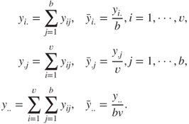
A few standard notations are in order. The ![]() treatment sample sum (mean), denoted by
treatment sample sum (mean), denoted by ![]() (
(![]() ) and total sample sum (mean),
) and total sample sum (mean), ![]() (
(![]() ), are defined by
), are defined by

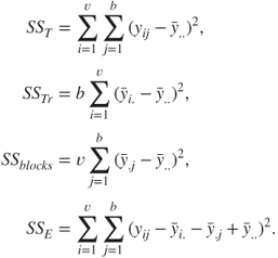
Define the total (corrected) sum of squares, denoted by ![]() , as
, as

The ANOVA technique partitions the ![]() as the sum of two components: (i) the sum of squares due to treatments
as the sum of two components: (i) the sum of squares due to treatments ![]() , and (ii) the sum of squares due to error
, and (ii) the sum of squares due to error ![]() . Here,
. Here, ![]() and
and ![]() are defined by
are defined by

Note that ![]() accounts for the between treatments effect, and
accounts for the between treatments effect, and ![]() accounts for the within treatments difference. Here,
accounts for the within treatments difference. Here, ![]() has
has ![]() degrees of freedom, whereas
degrees of freedom, whereas ![]() and
and ![]() have respectively
have respectively ![]() and
and ![]() degrees of freedom. It is easy to verify that
degrees of freedom. It is easy to verify that
Define
That is, ![]() is the sampling variance of the
is the sampling variance of the ![]() -th treatment. We can pool these
-th treatment. We can pool these ![]() sampling variances and obtain the following:
sampling variances and obtain the following:

where ![]() denotes the mean error sum of squares. Note that
denotes the mean error sum of squares. Note that ![]() is an estimator of the variance
is an estimator of the variance ![]() for the
for the ![]() -th treatment, and it may be seen that
-th treatment, and it may be seen that ![]() is an estimator of the common variance within each of the treatments. Similarly, we can also use the variation of the treatment averages from the grand average, under the assumption that there is no difference among the treatment means, for estimation of
is an estimator of the common variance within each of the treatments. Similarly, we can also use the variation of the treatment averages from the grand average, under the assumption that there is no difference among the treatment means, for estimation of ![]() . That is, the mean treatment sum of squares is given by
. That is, the mean treatment sum of squares is given by
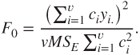
An interesting hypothesis testing problem is about the equality of effect of the treatment means: ![]() against the alternative
against the alternative ![]() . The details can then be presented in the ANOVA Table 13.2.
. The details can then be presented in the ANOVA Table 13.2.
Table 13.2 ANOVA for the CRD Model
| Source of Variation | Sum of Squares | Degrees of Freedom | Mean Square | |
| Between Treatments | ||||
| Error within Treatments | ||||
| Total |
In light of Theorem 6.6.2, the sampling distribution of ![]() and
and ![]() may be seen as an
may be seen as an ![]() -distribution with
-distribution with ![]() and
and ![]() degrees of freedom respectively. Finally, the sampling distribution of
degrees of freedom respectively. Finally, the sampling distribution of ![]() is seen to be an
is seen to be an ![]() -distribution, see Theorem 6.3.4, with
-distribution, see Theorem 6.3.4, with ![]() degrees of freedom.
degrees of freedom.
Before a formal illustration of the CRD model, let us take an EDA route for understanding ANOVA. The package granova has a very interesting graphical tool granova.1w, where 1w stands for “one-way layout”. The illustration through example(granova.1w) is first considered. The granova may be useful for outlier identification, skewness, etc.
In the next example, we will find out how R handles the covariates for the CRD model!
We will consider one more example for the CRD model 13.2 from Dean and Voss (1999).
Validation of the model assumptions is considered next.
13.3.4 Validation of Model Assumptions
The CRD model is a linear regression model, as in 12.1. The assumptions for the model are the same as detailed in Section 12.2, that is, linearity, independent, and normality assumptions. For the model under consideration, the plots, as in Section 12.2.6, give us all that is required. The demonstration is carried out for Example 13.3.3.
13.3.5 Contrasts and Multiple Testing for the CRD Model
Let us begin with a definition.
The statistical interest is in the problem of testing the hypothesis ![]() against the alternative
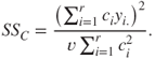
against the alternative ![]() . An estimate of the contrast
. An estimate of the contrast ![]() is given by
is given by
The test procedure is to reject ![]() if
if ![]() , where
, where
The test statistic ![]() is rewritten as
is rewritten as
where ![]() and
and ![]() is defined by
is defined by
Some contrasts are considered in the next example.
The problem of multiple testing was dealt with in Section 17.15. Here, the results are specialized to the CRD model.
If the hypothesis ![]() is rejected, we know that at least two treatment levels have significantly different effects. This calls for techniques which will help the reader to identify which treatments are significantly different. The details of the multiple comparison problem may be found in Miller (1981), Hsu (1996), and Bretz, et al. (2011).
is rejected, we know that at least two treatment levels have significantly different effects. This calls for techniques which will help the reader to identify which treatments are significantly different. The details of the multiple comparison problem may be found in Miller (1981), Hsu (1996), and Bretz, et al. (2011).
For the multiple testing problem we are familiar with the Bonferroni's method and the Holm's method. Tukey's honest significant differences, HSD, and Dunnett's procedures are detailed next.
In a CRD model with ![]() treatment levels, the interest is in comparison of the equality for each possible combination of the levels, that is, there are
treatment levels, the interest is in comparison of the equality for each possible combination of the levels, that is, there are ![]() possible hypotheses. Tukey's procedure uses the distribution of the Studentized range statistic:
possible hypotheses. Tukey's procedure uses the distribution of the Studentized range statistic:
where ![]() and
and ![]() are the largest and smallest sample means out of the
are the largest and smallest sample means out of the ![]() possible means. Tukey's HSD procedure declares two means to be significantly different if the absolute value of their differences exceeds
possible means. Tukey's HSD procedure declares two means to be significantly different if the absolute value of their differences exceeds
where ![]() is the upper
is the upper ![]() percentage point of
percentage point of ![]() and
and ![]() is the number of degrees of freedom associated with the
is the number of degrees of freedom associated with the ![]() . Thus, a
. Thus, a ![]() % confidence interval for all possible pairs of means is given by
% confidence interval for all possible pairs of means is given by
Suppose that one of the ![]() treatment levels is a control level and comparisons are required with respect to this control level. The Dunnett's procedure offers a solution in this case. The hypotheses are then
treatment levels is a control level and comparisons are required with respect to this control level. The Dunnett's procedure offers a solution in this case. The hypotheses are then ![]() , which then need to be tested against the set of hypotheses
, which then need to be tested against the set of hypotheses ![]() . The Dunnett's procedure begins with computation of the differences:
. The Dunnett's procedure begins with computation of the differences:
The test procedure is to reject the hypothesis ![]() at size
at size ![]() if
if
where ![]() corresponds to Dunnett's distribution.
corresponds to Dunnett's distribution.
The four methods of multiple testing are next illustrated for the tensile strength experiment.
The tensile strength experiment is an example of a balanced design. Fortunately, there is a slight change of ![]() , instead of the
, instead of the ![]() , but all the results continue to hold. In R there are no changes in the structure of the commands and functionality. Thus, the user can easily solve the multiple testing problem for the Olson dataset, which is an example of an unbalanced design.
, but all the results continue to hold. In R there are no changes in the structure of the commands and functionality. Thus, the user can easily solve the multiple testing problem for the Olson dataset, which is an example of an unbalanced design.
13.4 Block Designs
In the CRD model, the source of variation arises due to the different treatment levels. It is also assumed that the nuisance factor is completely unknown and uncontrollable. In the case of the nuisance factor being known and controllable, the experiment can be designed to account for such a source of error through blocking.
13.4.1 Randomization and Analysis of Balanced Block Designs
In a block model, a comparison needs to be carried out for the different treatment levels and blocks. In a balanced block design, each block will have one observation per treatment level. It is to be noted that randomization is only carried out on the treatments within a block. The effects model for a balanced block design model is specified by
where ![]() is the overall mean,
is the overall mean, ![]() is the effect of the
is the effect of the ![]() -th treatment, and
-th treatment, and ![]() is the effect of the
is the effect of the ![]() -th block. Also, define
-th block. Also, define ![]() . As previously we assume that the error term
. As previously we assume that the error term ![]() follows a Gaussian distribution
follows a Gaussian distribution ![]() .
.
The randomization for the above design 13.10 is illustrated next.
Towards inference for the randomized block design, define the following quantities:
The decomposition of the total sum of squares ![]() is given below:
is given below:
where
Observe that ![]() has
has ![]() degrees of freedom,
degrees of freedom, ![]() has
has ![]() df,
df, ![]() has
has ![]() df, and finally,
df, and finally, ![]() has
has ![]() df. Thus, the ANOVA table is then set up as given in Table 13.3. The balanced block design will be illustrated now.
df. Thus, the ANOVA table is then set up as given in Table 13.3. The balanced block design will be illustrated now.
Table 13.3 ANOVA for the Randomized Balanced Block Model
| Source of Variation | Sum of Squares | Degrees of Freedom | Mean Square | |
| Between Treatments | ||||
| Between Blocks | ||||
| Error | ||||
| Total |
As seen in Models 13.2, 13.10, etc., these linear models need to be investigated for model assumptions and other regression diagnostics too. Can it be said without loss of generality that leverages are not a concern in DOE since all the covariate values are fixed? Now, we consider an example from Montgomery (2005), wherein we will investigate issues related to model adequacy.
13.4.2 Incomplete Block Designs
The constraints of the real world may not allow each block to have an experimental unit for every treatment level. The restriction may force allocation of only ![]() units within each block. Such models are called incomplete block designs. If in an incomplete block design, any two treatments pair appearing together, across the blocks, occurring an equal number of times, the designs are then called balanced incomplete block designs, abbreviated as BIBD. It may be seen that a BIBD may be constructed in
units within each block. Such models are called incomplete block designs. If in an incomplete block design, any two treatments pair appearing together, across the blocks, occurring an equal number of times, the designs are then called balanced incomplete block designs, abbreviated as BIBD. It may be seen that a BIBD may be constructed in ![]() different ways.
different ways.
The setup is now recollected again. We have ![]() treatments,
treatments, ![]() distinct blocks,
distinct blocks, ![]() is the number of units appearing in a block, and
is the number of units appearing in a block, and ![]() is the total number of observations, where
is the total number of observations, where ![]() is the number of times a treatment appears in the design. Then, the number of times each pair of treatments appears in the same block is given by
is the number of times a treatment appears in the design. Then, the number of times each pair of treatments appears in the same block is given by
The statistical model for BIBD is given by
where ![]() is the
is the ![]() observation in the
observation in the ![]() block,
block, ![]() is the overall mean,
is the overall mean, ![]() is the effect of the
is the effect of the ![]() treatment, and
treatment, and ![]() is the effect of the
is the effect of the ![]() block. The error term
block. The error term ![]() is assumed to follow
is assumed to follow ![]() . The total variability needs to be handled in a slightly different manner. Define
. The total variability needs to be handled in a slightly different manner. Define
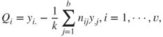
where
Using the ![]() 's, the adjusted treatment sum of squares is defined by
's, the adjusted treatment sum of squares is defined by
Thus, the total variability is partitioned by
where

The ANOVA table for BIBD model is given in Table 13.4.
Table 13.4 ANOVA for the BIBD Model
| Source of Variation | Sum of Squares | Degrees of Freedom | Mean Square | |
| Between Treatments | ||||
| Between Blocks | ||||
| Error | ||||
| Total |
The function BIB.test from the agricolae package is useful to fit a BIBD model.
Two very important variations of the BIBD will be considered in the rest of the section.
13.4.3 Latin Square Design
In each of the Examples 13.4.1 to 13.4.4, and the blocking models 13.2 and 13.10, we had a single source of known and controllable source of variation and we use the blocking principle to overcome this. Suppose now that there are two ways or sources of the variation which may be controlled through blocking! Consider the following example from Montgomery (2001), page 144.
In the above example, we need to ensure that each type of formulation occurs exactly once for the type of raw material and also that each formulation is prepared exactly once by each of the five operators. This type of problem is handled by the Latin Square Design, abbreviated as LSD, and we use the Latin letters to represent the type of formulations. A simple technique is to set up an LSD for say ![]() formulations, set up in the first row of the design as 1, 2, …,
formulations, set up in the first row of the design as 1, 2, …, ![]() , the second row as 2, 3, …,
, the second row as 2, 3, …, ![]() ,1, the third row as 3, 4, …,
,1, the third row as 3, 4, …, ![]() , 2, 1, and so forth until the last row as
, 2, 1, and so forth until the last row as ![]() ,
, ![]() , …, 3, 2, 1. There are many other techniques available for creating an LSD, such as Wichmann-Hill, Marsaglia-Multicarry, Mersenne-Twister, Super-Duper, etc. A couple of illustrations are given next using the
, …, 3, 2, 1. There are many other techniques available for creating an LSD, such as Wichmann-Hill, Marsaglia-Multicarry, Mersenne-Twister, Super-Duper, etc. A couple of illustrations are given next using the design.lsd function from the agricolae package.
The LSD model and its statistical analyses is now detailed. The LSD statistical model is specified by
Here, ![]() will continue to represent the effect of the
will continue to represent the effect of the ![]() -th treatment (or formulation),
-th treatment (or formulation), ![]() for the row (block) effect (raw material), and
for the row (block) effect (raw material), and ![]() for the column (block) effect (operator). The errors are assumed to follow normal distribution
for the column (block) effect (operator). The errors are assumed to follow normal distribution ![]() . The ANOVA decomposition of the sum of squares for the LSD model 13.16 will be as follows:
. The ANOVA decomposition of the sum of squares for the LSD model 13.16 will be as follows:
where

The ANOVA table for the LSD is given in Table 13.5. For Example 13.4.5, the R method is illustrated next.
Table 13.5 ANOVA for the LSD Model
| Source of Variation | Sum of Squares | Degrees of Freedom | Mean Square | |
| Between Treatments | ||||
| Between Rows | ||||
| Between Columns | ||||
| Error | ||||
| Total |
There are many other useful variants of LSD and the reader may refer to Chapter 10 of Hinkelmann and Kempthorne (2008) for the same. An extension of the LSD is considered in the next topic.
13.4.4 Graeco Latin Square Design
Suppose that there is an extra source of randomness for the Rocket Propellant problem in Example 13.4.5 in test assemblies, which forms an additional type of treatment. Now, it is obvious that this is a second treatment which may be again addressed by another LSD. Let us denote the second treatment by Greek letters, say ![]() ,
, ![]() ,
, ![]() ,
, ![]() , and
, and ![]() . There is symbolic confusion in the sense that the Greek letters of
. There is symbolic confusion in the sense that the Greek letters of ![]() ,
, ![]() , and
, and ![]() may be confused with the notations used in Model 13.16. However, we will use the notations as elements of the LSD matrix. It should be clear from the context whether the notations are as in the Greek letters required or in the statistical model. Now, the LSD matrices for the two treatments are superimposed on each other to obtain the Graeco-Latin Square Design model. Table 13.6 shows how superimposing is done for two simple LSDs to obtain the GLSD.
may be confused with the notations used in Model 13.16. However, we will use the notations as elements of the LSD matrix. It should be clear from the context whether the notations are as in the Greek letters required or in the statistical model. Now, the LSD matrices for the two treatments are superimposed on each other to obtain the Graeco-Latin Square Design model. Table 13.6 shows how superimposing is done for two simple LSDs to obtain the GLSD.
Table 13.6 The GLSD Model
| LSD | GSD | GLSD | ||||||
| A | B | C | A |
B |
C |
|||
| B | C | A | B |
C |
A |
|||
| C | A | B | C |
A |
B |
|||
In more formal terms, the Graeco-Latin square design model, abbreviated as GLSD, is specified by
where ![]() now denotes the effect of the additional treatment. A couple of GLSDs will be first set up.
now denotes the effect of the additional treatment. A couple of GLSDs will be first set up.
The ANOVA decomposition of the sum of squares for the GLSD model 13.18 will be as follows:
where
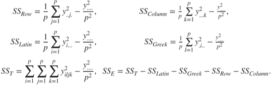
The ANOVA table for the GLSD is given in Table 13.7. For Example 13.4.5, the R method is illustrated next.
Table 13.7 ANOVA for the GLSD Model
| Source of Variation | Sum of Squares | Degrees of Freedom | Mean Square | |
| Between Latin Treatments | ||||
| Between Greek Treatments | ||||
| Between Rows | ||||
| Between Columns | ||||
| Error | ||||
| Total |
We now move to more important and complex experimental designs.
13.5 Factorial Designs
Factorial designs1 are useful in experiments involving two or more factor variables. Suppose that there are two factor variables, with variable 1 having ![]() levels and variable 2 having
levels and variable 2 having ![]() levels. A factorial design investigates all possible combinations of the levels of the factors. In simple words, if factor
levels. A factorial design investigates all possible combinations of the levels of the factors. In simple words, if factor ![]() is at
is at ![]() levels, factor
levels, factor ![]() at
at ![]() levels, and factor
levels, and factor ![]() at
at ![]() levels, a factorial design will investigate all possible levels
levels, a factorial design will investigate all possible levels ![]() . It is then common practice to say that factors are crossed, implying that each factor variable level also has a corresponding observation among the levels of other factors. In factorial designs, the interest is more often to determine if there is an interaction between some combination of the factor levels. What does interaction really mean? In general, the main effects of a factor are observed to be the changes in the regressand due to the changes of the factor levels. However, if the changes in such expected values of the regressand also depend on the levels of other factor variables, we believe that there is an interaction effect between the factor variables. In the previously discussed designs in Sections 13.3 and 13.4, the factors were implicitly assumed to not have any kind of interaction among their different levels. Recollect from the three-dimensional scatter plot in Figure 12.6 and the cantor plot in Figure 12.7, the model 12.31 consisted of straight lines or planes only. However, for the models 12.31 and Figure 13.6, the three-dimensional plots and cantor plots had curvi-linear shapes in them, which is then an indication of the presence of interaction among the variables.
. It is then common practice to say that factors are crossed, implying that each factor variable level also has a corresponding observation among the levels of other factors. In factorial designs, the interest is more often to determine if there is an interaction between some combination of the factor levels. What does interaction really mean? In general, the main effects of a factor are observed to be the changes in the regressand due to the changes of the factor levels. However, if the changes in such expected values of the regressand also depend on the levels of other factor variables, we believe that there is an interaction effect between the factor variables. In the previously discussed designs in Sections 13.3 and 13.4, the factors were implicitly assumed to not have any kind of interaction among their different levels. Recollect from the three-dimensional scatter plot in Figure 12.6 and the cantor plot in Figure 12.7, the model 12.31 consisted of straight lines or planes only. However, for the models 12.31 and Figure 13.6, the three-dimensional plots and cantor plots had curvi-linear shapes in them, which is then an indication of the presence of interaction among the variables.
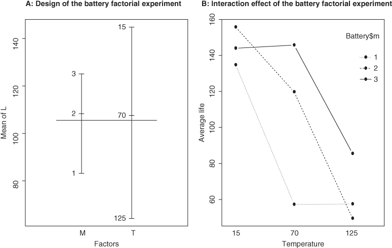
Figure 13.6 Design and Interaction Plots for 2-Factorial Design
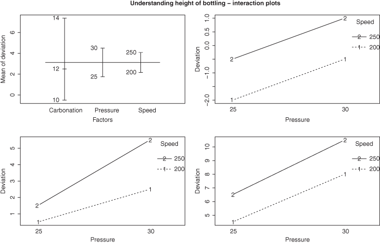
Figure 13.7 Understanding Interactions for the Bottling Experiment
Sir R.A. Fisher advocated the use of a complex design like factorial designs with “No aphorism is more frequently repeated in connection with field trials, than that we must ask Nature a few questions, or, ideally, one question, at a time. The writer is convinced that this view is wholly mistaken.” To understand this advantage, consider two factorial variables at two levels each. Suppose that two factor variables, ![]() and
and ![]() , are both available at levels high
, are both available at levels high ![]() and low
and low ![]() . Then the four possible combinations of the two treatments are
. Then the four possible combinations of the two treatments are ![]() ,
, ![]() ,
, ![]() , and
, and ![]() . If low refers to the absence of factor levels, it is also a common practice to denote these respective combination levels with
. If low refers to the absence of factor levels, it is also a common practice to denote these respective combination levels with ![]() ,
, ![]() ,
, ![]() , and
, and ![]() . Suppose we are interested in finding the effect of changing the factors
. Suppose we are interested in finding the effect of changing the factors ![]() and
and ![]() . A rule of thumb is to take two observations at each combination level of the factors in the presence of the experimental error. Now, the effect of treatment factor
. A rule of thumb is to take two observations at each combination level of the factors in the presence of the experimental error. Now, the effect of treatment factor ![]() is found by the difference in the combination level of
is found by the difference in the combination level of ![]() , while that of
, while that of ![]() is with
is with ![]() . Thus, we require data on the three combination levels
. Thus, we require data on the three combination levels ![]() ,
, ![]() , and
, and ![]() , or equivalently six observations only. In a full factorial experiment, we would also have two more data points at the combination level
, or equivalently six observations only. In a full factorial experiment, we would also have two more data points at the combination level ![]() . Now, we can obtain two main effects for
. Now, we can obtain two main effects for ![]() with
with ![]() and
and ![]() , and two main effects for
, and two main effects for ![]() too with
too with ![]() and
and ![]() .
.
In the remainder of this section, we will consider some useful factorial designs. The focus will be only on fixed effects models.
13.5.1 Two Factorial Experiment
Consider the case of two factor variables. Suppose that factor ![]() is at
is at ![]() levels, and
levels, and ![]() at
at ![]() levels. The two factorial design model is given by
levels. The two factorial design model is given by
Here, ![]() is the overall mean effect,
is the overall mean effect, ![]() is the effect of the
is the effect of the ![]() -th factor level of
-th factor level of ![]() ,
, ![]() is the
is the ![]() -th effect of the factor
-th effect of the factor ![]() , and
, and ![]() is the interaction effect between the variables. The ANOVA decomposition of the sum of squares for the two factorial experiments is given by
is the interaction effect between the variables. The ANOVA decomposition of the sum of squares for the two factorial experiments is given by
where

The computation of ![]() involves two stages. Since such issues do not exist when we use R, we skip this detail. The ANOVA table for the two-factorial model is given in Table 13.8. The hypotheses problems of interest here are the following:
involves two stages. Since such issues do not exist when we use R, we skip this detail. The ANOVA table for the two-factorial model is given in Table 13.8. The hypotheses problems of interest here are the following:
- 1. Testing for Factor
 :
:
- 2. Testing for Factor
 :
:
- 3. Testing for the Interaction of factors:

Table 13.8 ANOVA for the Two Factorial Model
| Source of Variation | Sum of Squares | Degrees of Freedom | Mean Square | |
| Treatment A | ||||
| Treatment B | ||||
| Interaction | ||||
| Error | ||||
| Total |
The two-factorial experiment is now illustrated with an example from Montgomery (2005).
The extension of the two-factorial experiment is discussed in the next subsection.
13.5.2 Three-Factorial Experiment
A natural extension of the two-factorial experiment will be the three-factorial experiment. Let the three factors be denoted by ![]() ,
, ![]() , and
, and ![]() , each respectively at
, each respectively at ![]() ,
, ![]() , and
, and ![]() factor levels. Consequently, there are now three more interaction terms to be modeled for in
factor levels. Consequently, there are now three more interaction terms to be modeled for in ![]() ,
, ![]() , and
, and ![]() . Towards a complete crossed model, we need each replicate (of index
. Towards a complete crossed model, we need each replicate (of index ![]() ) to cover all possible factor combinations. Thus, the three-way factorial model is then modeled by
) to cover all possible factor combinations. Thus, the three-way factorial model is then modeled by
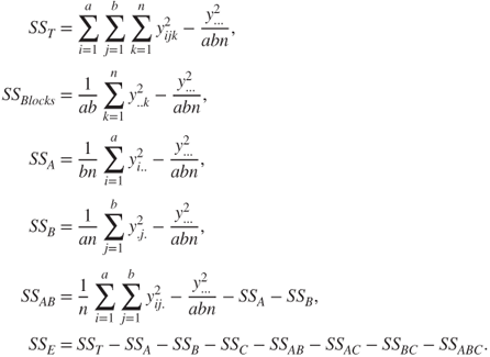
The total sum of squares decomposition equation is then
where

The ANOVA table for the three-factorial design model is given in Table 13.9.
Table 13.9 ANOVA for the Three-Factorial Model
| Source of Variation | Sum of Squares | Degrees of Freedom | Mean Square | |
| Treatment A | ||||
| Treatment B | ||||
| Treatment C | ||||
| Interaction (AB) | ||||
| Interaction (AC) | ||||
| Interaction (BC) | ||||
| Interaction (ABC) | ||||
| Error | ||||
| Total |
Since the details of the two-factorial experiment extend in a fairly straightforward manner to the current model, the model will be illustrated with two examples from Montgomery (2005).
The principle of blocking in the context of factorial experiments is taken up in the next subsection.
13.5.3 Blocking in Factorial Experiments
The two- and three-factorial experiments discussed above are extensions of the basic CRD model. In Section 13.4, we saw that replication does not alone eliminate the source of error and that the principle of blocking helps improve the efficiency of the experiment. Similarly, in the case of factorial experiments, practical considerations sometimes dictate that the replication principle cannot be implemented uniformly and that the factorial experiments may be improved through the introduction of a blocking route. The blocking model for a two-factorial experiment is stated next:
The total sum of squares decomposition equation for the model 13.24 is then
where
The corresponding ANOVA table for the blocking factorial experiment 13.24 is given in Table 13.10.
Table 13.10 ANOVA for Factorial Models with Blocking
| Source of Variation | Sum of Squares | Degrees of Freedom | Mean Square | |
| Blocks | ||||
| Treatment A | ||||
| Treatment B | ||||
| Interaction (AB) | ||||
| Error | ||||
| Total |
The theory and applications of Experimental Designs extend far beyond the models discussed here and thankfully the purpose of the current chapter has been to consider some of the important models among them.
13.6 Further Reading
Kempthorne (1952), Cochran and Cox (1958), Box, Hunter, and Hunter (2005), Federer (1955), and of course, Fisher (1971) are some of the earliest treatises in this area.
Montgomery (2005), Wu and Hamada (2000–9), and Dean and Voss (1999) are some of the modern accounts in DOE. Casella (2008) is a very useful source with emphasis on computations using R. The web link http://cran.r-project.org/web/views/ExperimentalDesign.html is very useful for the reader interested in almost exhaustive options for DOE analysis using R.
13.7 Complements, Problems, and Programs
Problem 13.1 Identify which of the design models studied in this chapter are appropriate for the datasets available in the
BHH2package. The list of datasets available in the package may be found withtry(data(package="BHH2")). The exercise may also be repeated for design-related packages such asagricolae,AlgDesign, andgranova.Problem 13.2 Carry out the diagnostic tests for the
olson_crdfitted model in Example 13.3.4. Repeat a similar exercise for the ANOVA model fitted in Example 13.3.2.Problem 13.3 Multiple comparison tests of Dunnett, Tukey, Holm, and Bonferroni have been explored in Example 13.3.8. The confidence intervals are reported only for
TukeyHSD. The reader should obtain the confidence intervals for the rest of the multiple comparison tests contrasts.Problem 13.4 Explore the use of the functions
design.crdanddesign.rcbdfrom theagricolaepackage for setting up CRD and block designs.Problem 13.5 The function
granova.2wmay be applied on thegirdernewdataset with a slight modification. Create a new data framegirdernew2 <- girdernew[,c(3,1,2)]. Note that an additional R packagerglwill be required though. Test the codegranova.2w( girdernew2,ss gf + mf)and make an attempt to interpret the output.Problem 13.6 In the fitted models
ssaov,hardness_aov,rocket_aov,rocket.aov, androcket.glsd.aovdiscussed in Section 13.4, investigate the presence of an interaction effect through the use of theinteraction.plotgraphical function.Problem 13.7 Perform the diagnostic tests on the BIBD model in Example 13.4.4.
Problem 13.8 Investigate the presence of outliers and influential measures for the fitted models
rocket.lmandrocket.glsd.lmin the respective Examples 13.4.7 and 13.4.9.Problem 13.9 Obtain the confidence intervals for the contrasts of the fitted model
battery.aovin Example 13.5.1.Problem 13.10 Carry out the diagnostic tests for the fitted models
bottling.aov,SP.aov, andintensity.aov.