In Chapter 4 we came across one form of analyzing data, viz., the exploratory data analysis. That approach mainly made no assumptions about the probability mechanism for the data generation. In later chapters we witnessed certain models which plausibly explain the nature of the random phenomenon. In reality, we seldom have information about the parameters of the probability distributions. Historically, or intuitively, we may have enough information about the probability distributions, sparing a few parameters. In this chapter we consider various methods for inferring about such parameters, using the data generated under the assumptions of these probability models.
Parametric statistical inference arises when we have information for the model describing an uncertain experiment sans a few values, called parameters, of the model. If the parameter values are known, we have problems more of the probabilistic kind than statistical ones. The parameter values need to be obtained based on some data. The data may be a pure random sample in the sense of all the observations being drawn with the same probability. However, it is also the practical case that obtaining a random sample may not be possible in many stochastic experiments. For example, the temperature in the morning and afternoon are certainly not identical observations. We undertake statistical inference of uncertain experiments in this chapter.
In Chapter 6, we came across a pool of diverse experiments which have certain underlying probability models, say . Under the assumption that is the truth, we now develop methods for inference about . We will begin with some important families of distribution in Section 7.2. This section and the next few sections rely heavily on Lehmann and Casella (1998). The form of loss functions plays a vital role on the usefulness of an estimator/statistic. For an observation from binomial distribution, we discuss some choice of loss functions in Section 7.3. Data reduction through the concepts of sufficiency and completeness are theoretically examined in Section 7.4. Section 7.5 empathizes the importance of the likelihood principle through visualization and examples. The role of information function for obtaining the parameter values is also detailed in this section. The discussion thus far focuses on the preliminaries of point estimation.
Using the foundations from Sections 7.2–7.5, we next focus on the specific techniques of obtaining the estimates of parameters using maximum likelihood estimator and moment estimator in Section 7.6. Estimators are further compared for their unbiasedness and variance in Section 7.7. The techniques discussed up to this point of the chapter return us a single value of the parameter, which is seldom useful in appropriating inference for the parameters. Thus, we seek a range, actually interval, of plausible values of the parameters in Section 7.8. In the case of missing values, or a data structure which may be simplified through missing variables, the EM algorithm is becoming very popular and the reader will find it illustrated in Section 7.16.
Sections 7.9–7.15 offers a transparent approach to the problem of Testing Statistical Hypotheses. It is common for statistical software texts to focus on the testing framework using straightforward useful R functions available in prop.test, t.test, etc. However, here we take a pedagogical approach and begin with preliminary concepts of Type I and Type II errors. The celebrated Neyman-Pearson lemma is stated and then demonstrated for various examples with R programs in Section 7.10. The Neyman-Pearson lemma returns us to a unique powerful test which cannot be extended for testing problems of composite hypotheses, and thus we need slightly relaxed conditions leading to uniformly most powerful tests and also uniformly most powerful unbiased tests, as seen in Sections 7.11 and 7.12. A more generic class of useful tests is available in the family of likelihood ratio tests. Its examples are detailed with R programs in Section 7.13. A very interesting problem, which is still unsolved, arises in the comparison of normal means from two populations whose variances are completely unknown. This famous Behrens-Fisher problem is discussed with appropriate solutions in Section 7.14. The last technical section of the chapter deals with the problem of testing multiple hypotheses, Section 7.15.
7.2 Families of Distribution
We will begin with a definition of a group family, page 17 of Lehmann and Casella (1998).
The identity element of a group and the inverses of any element are unique. The two important properties of a group are (i) closure under composition, and (ii) closure under inversion. Basically, for various reasons, we change the characteristics of random variables by either adding them, or addition or multiplication of some constants, etc. We need some assurance that such changes do not render the probability model from which we started useless. The changes which we subject the random variable to is loosely referred to as a transformation. Let us discuss these two properties in more detail.
Closure under composition. A 1:1 transformation may be addition or multiplication. We say that a class of transformation is closed under composition if implies .
Closure under inversion. For any 1:1 transformation , the inverse of , denoted by , undoes the transformation , that is, . A class of transformations is said to be closed under inversion if for any , the inverse is also in .
In plain words, if a random variable under a group family is subject to a transformation, the resulting distribution also belongs to the same class of distribution. The transformation may include addition, multiplication, sine, etc.
Table 4.1 of Lehmann and Casella (1998) gives an important list of location-scale families.
7.2.1 The Exponential Family
The canonical form is not necessarily unique.
Note that we speak of a family of probability distributions belonging to an exponential family, and as such we are not focusing on a single density, say .
7.2.2 Pitman Family
The exponential family meets the regularity condition since the range of random variable is not a function of the parameter . In many interesting cases, the range of the random variable depends on a function of its parameters. In such cases the regularity condition is not satisfied. A nice discussion about such non-regular random variables appears on Page 19 of Srivastava and Srivastava (2009).
The mathematical argument is as follows. Let be a positive function of and let and , be the extended real-valued functions of parameter . We can then define a density by
7.6
where
Thus, we can see that the range of depends on , and hence the density is a non-regular. The family of such densities is referred to as the Pitman family. In Table 7.1, a list of some members of the Pitman family is provided, refer to Table 1.3 of Srivastava and Srivastava (2009).
A statistic, or an estimator, is employed for estimation of a parameter, say . The loss incurred as a consequence of using is captured using a loss function. In convention with the standard notation, the loss function of a parameter inferred by using will be denoted by . Some useful loss functions are now given.
In this section we will consider the squared error loss function only. To evaluate the performance of an estimator under a loss function , we require the notion of risk function defined as
7.7
For a fixed , calculates the risk of using the statistic . The risk function is the average loss due to . The risk function under the squared error loss functions is also popularly known as the mean squared error of the estimator. The next example illustrates the risk function for four different statistics . Since also leads more often to making some decisions, we sometimes also denote the statistic by . In fact, the loss functions have a more prominent role in decision theory.
The role of loss functions will become more prominent in Section 7.7. The section will be closed with an interesting example where the degenerate estimator is to be preferred over a reasonable estimator.
7.4 Data Reduction
Statistical inference has two very important pillars: (i) The Sufficiency Principle, and (ii) The Likelihood Principle. Berger and Woolpert (1988) is a treatise for understanding these principles. In this section we will consider the sufficiency principle in depth.
7.4.1 Sufficiency
It is seen in Section 7.3 that many possible statistics exist for a given parameter. Some statistics have an advantage over others and a meaningful criteria needs to be arrived at to help in these type of decisions.
Thus far we began with statistics and verified whether it satisfied the sufficiency condition. It is not always possible to guess what may turn out to be sufficient statistics. The Neyman Factorization theorem gives a result which helps to obtain the sufficient statistics from the joint probability function of the random sample. A measure theoretic framework of this theorem is due to Halmos and Savage (1949), see page 289 of Mukhopadhyay (2000) for more details. The following theorem may be found in Casella and Berger (2002).
We will now use this result to obtain the sufficient statistics in some important cases.
If in the previous example is known, it can be seen that , , , and other permutations are all sufficient for . Thus, we need a more general framework to identify the sufficient statistics. Furthermore, there may be more than one sufficient statistic and in such cases we need to pick one among them.
7.4.2 Minimal Sufficiency
Dynkin (1951) gave the criteria for a statistic to be necessary.
In the discussion before this subsection, it can be seen that the statistics can be mathematically written as a function of and . Thus, if , , and are the only three sufficient statistics, though there are many more sufficient statistics in the scenario, then turns out to be a necessary statistic. This definition further guides towards the concept of minimal sufficient statistics.
It is not practical to obtain a minimal sufficient statistic from its definition. Lehmann and Scheffé (1950) provide a result which is useful in obtaining a minimal sufficient statistic. We first describe this important result.
A useful result states that a complete sufficient statistic will be minimal and hence if the completeness of the sufficient statistic can be established, it will be minimal sufficient too. In the case of the exponential families of full rank, the statistic will be a complete statistic. We had already seen that is also sufficient, and hence for exponential families of full rank, it will be minimal sufficient. Since the examples of gamma, Poisson, etc., are members of an exponential family with full rank, the sufficient estimators/statistics seen earlier will be complete, and hence minimal sufficient too. The likelihood principle is developed in the next section.
7.5 Likelihood and Information
As mentioned at the beginning of the previous section, we will now consider the second important principle in the theory of statistical inference: the likelihood principle. The likelihood function is first defined.
7.5.1 The Likelihood Principle
A major difference between the likelihood function and (joint) pdf needs to be emphasized. In a pdf (or pmf), we know the parameters and try to make certain probability statements about the random variable. In the likelihood function the parameters are unknown and hence we use the data to infer certain aspects of the parameters. In simple and practical terms, we generally plot the pdf against values to understand it, whereas for the likelihood function plots, we plot against the parameter . Obviously there is more to it than what we have simply said here, though what is detailed here suffices to understand the likelihood principle. Furthermore, it has been observed that many books lay far more emphasis on the maximum likelihood estimator, to be introduced in the Section 7.6, and the primary likelihood function is given a formal introduction. Barnard, et al. (1962) have been emphatic about the importance of the likelihood function. Pawitan (2001) is another excellent source for understanding the importance of likelihood. Moreover, Pawitan also provides R codes and functions towards understanding this principle. Naturally, this section is influenced by his book.
The likelihood function contains more information about the data and the parameters than some summary measures of the data. Plots of the likelihood, whenever possible, throw more light on random phenomenon and should be employed in as many cases as they permit. We will now formally state the likelihood principle.
More formal use of the likelihood function will be explained in the forthcoming subsection.
7.5.2 The Fisher Information
The likelihood function will now be more formally used towards the inference of the parameters. We will first define the score function.
The natural question is how do we make use of the score function as given in Equation 7.15. We will first begin with an illustration of the sampling variance of score functions.
An important exercise is to prove that the expectation of the score function equals zero, that is, , which we leave to the reader.
In the above definition, the term partial derivative has been used in the sense that the parameter may be a vector and in which case we consider the derivative of the likelihood function with respect to each component of the vector.
A useful result regarding the expected Fisher information, under the assumptions of the regularity conditions of course, is
We will next find the Fisher information for a few well-known probability distributions.
The next result is an important one when we have to calculate the Fisher information for a random sample.
In the next section we will use the observed Fisher information in a random sample.
7.6 Point Estimation
“Point Estimation” or “Estimation Theory” are some of the common names for dealing with the problem of estimation of parameters. Lehmann and Casella (1998) is one of the best sources for classical inference. Modern accounts of this domain are Casella and Berger (2002), Shao (2003), and Mukhopadhyay (2000). For details about the maximum likelihood technique implementation, refer to Millar (2011).
7.6.1 Maximum Likelihood Estimation
In the previous section we introduced the likelihood function. It will now be used to find estimators.
Let be a random sample with common pdf or pmf , . The random variable and/or may be scalar or vector. Recall the definition of likelihood function:
It is important to note that the MLE definition simply requires that the likelihood function be optimized. There is no specific method outlined on how to obtain the MLE. We will begin with a few graphical methods, which will be a continuation of some of our earlier examples.
We will now attempt to obtain the MLEs when the parameters are continuous. A standard technique in calculus for obtaining the optimum value of a continuous function is by differentiating the function with respect to the continuous variable and setting the resultant expression to zero. In our case, such an expression turns out to be the score function which we saw in the previous Section 7.5. The MLE is then a root (solution) of the score function, that is, a solution of the equation:
Note that in each of the four score function plots in Figure 7.4, the parameter values which correspond to the score function at 0 is 4. This is not surprising since we had simulated the datasets to have the average (mean) of 4 only. Let us verify again with a plot of the score function for the normal sample and check if the plot helps to find the MLE in the spirit of Pawitan (2001).
Setting the score functions equal to zero, and then obtaining an appropriate expression for the parameters, will give us estimators of the likelihood function, that is, the MLE. For the score-functions given in Equations 7.16–7.18, we obtain the MLEs by solving them as follows:
7.23
7.24
7.25
To be assured that , , and as given above, are indeed the MLEs, we need to look at the derivatives of the score function and verify that they are negative. The derivatives of the score functions for the distributions are stated next:
The derivatives of the log-likelihood function for normal and Poisson distribution, Equations 7.26 and 7.27, may easily be understood as negative, whereas it is not straightforward to obtain the answer for binomial and Cauchy distributions. In the binomial case, the reader may refer to a slightly different case at http://www.montana.edu/rotella/502/binom_like.pdf.
Note that the MLE for the Cauchy distribution has not been derived here and it requires a different way of solving the score function to obtain the MLE. We will be using three functions available in R, optimize, mle and nlm for obtaining the MLEs. Since we have emphasized the likelihood function, it is always good practice to report the values of the likelihood function, or its variants such as the log-likelihood function, or negative of the log-likelihood function.
The Cauchy distribution is slightly more complex and its MLE does not exist in a simple form. We resort to the numerical optimization technique, essentially the Newton-Raphson technique, through its score function as given in Equation 7.19.
The MLE problems, and likelihood functions as well, thus far has been discussed in the context of a single unknown parameter only. In many applied contexts, it is a common theme that multiple parameters would be unknown. The approach remains the same, though the details will be obviously more. Let us consider a random sample from the normal distribution, where both the parameters and are unknown. Recollect that in Example 7.5.5 we had assumed .
We will close this sub-section with a very interesting example.
We will close this discussion with some properties of the MLE.
1. If is a sufficient statistic for the family of distributions and a unique MLE of exists, then the MLE is a function of the sufficient statistic .
2. If is an MLE for and is a one-to-one function of , then will be an MLE for .
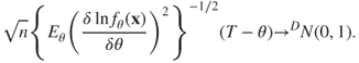
3. Under certain regularity conditions, see Section 7.7, the MLE is a consistent estimator, and further
7.33
7.6.2 Method of Moments Estimator
Karl Pearson invented the method of moments estimator. Suppose that is the pmf (pdf), and that the parameters are in number, . The method of moments estimator means that we need to first find the theoretical moments of and assume that they are equal to the corresponding sample moments. We assume that we have a sample of size . Thus, we have equations for unknown quantities. A solution for this set of equations leads to the method of moments estimator. Symbolically, we have the following setup:
We will demonstrate the applications of the moment estimators through some examples of Mukhopadhyay (2000) and Casella and Berger (2002). An important point to note here is that the moment estimators can be computed. even if the complete density function is not known.
However, it is to be noted that the moment estimator is an ad hoc solution for obtaining estimators and it is severely restricted. Please refer to Mukhopadhyay (2000) and Casella and Berger (2002) for more pointers in this regard.
7.7 Comparison of Estimators
In the previous sections we considered two main methods of estimation. It is possible to propose several estimators for the same parameter and we would have to then justify the use of one estimator over other. That is, we need criteria for comparison of estimators. We will begin with unbiased estimator as a criterion for comparison purposes.
7.7.1 Unbiased Estimators
It needs to be recorded that the lack of bias is a property of an estimator and not of a sample. An unbiased estimator reaches the target on average and its bias will be 0 for all values of . An important measure of the performance of a statistic is provided by its Mean Squared Error.
A result which connects variance, bias, and MSE is given next.
In the previous Example 7.7.1, we had four unbiased estimators . Among these we will prefer the estimator with the least variance. This leads to the following definition.
In the following, we will first consider improving the unbiased estimators using sufficient statistics via the Rao-Blackwellization process. Next we will state what will be the lower bound for variance of unbiased estimators using Cramér-Rao inequality. Finally, we will briefly discuss how to obtain UMVU estimators.
7.7.2 Improving Unbiased Estimators
If we have an unbiased estimator, and we seek an improvement of it in terms of reduction in variance, we have an affirmative answer in the Rao-Blackwell theorem.
An illustration of how the Rao-Blackwell theorem works is required here.
The reader may consult Mukhopadhyay (2000) for more interesting examples of Rao-Blackwellization. We have taken one important step towards reducing the variance via sufficiency and we should now ask what is the best we can do further. Under some mild regularity conditions, the answer is provided by Cramér-Rao's lower bound. We need the following assumptions.
a. The support of is independent of .
b. exists .
c..
d..
e..
As the above inequality involves the Fisher information, Lehmann and Casella (1998) refer to the Cramér-Rao inequality as the information inequality. The Cramér-Rao inequality can be derived using the characteristic function, see Kay and Xu (2008).
We will close this section with an important result which leads towards deriving UMVUE for some special family of probability distributions.
7.8 Confidence Intervals
Point estimates of the parameters are useful as already seen. However, there is often a need to complement them with other techniques, and a very brief discussion on the technique of confidence intervals will be discussed here. It is admitted that this topic requires more depth, and is restricted only in part by the important problem of hypotheses testing, which is covered in a more rigorous and R way. Another reason for skipping over the details on confidence intervals in part is that most of the R statistical functions, the confidence intervals, are also provided as part of the output when we use the well-known tests. In fact, the R function confint is also available, which extracts the confidence intervals with desired confidence widths for the regression models.
The reader may refer Chapter 5 of Tattar (2013) for confidence interval functions binom_CI, normal_CI_ksd, and normal_CI_uksd. Chapter 8 of Ugarte, et al. (2008) is a comprehensive account of the confidence intervals construction in R. A reason for not developing this section in more detail is that most of the statistical tests in R such as t.test, var.test, binom.test give the confidence intervals as side products in the output. Furthermore, the function confint is applicable to many statistical models fitted in R.
In earlier sections we explored various techniques of estimating the unknown parameters. The next task is validation of these parameters. Especially, we would like to deduce if the estimated parameters are in agreement with certain conjectures. We will now introduce some important terminology.
Consider a random sample whose underlying probability law is a pmf or a pdf .
Testing the hypotheses problem is the statistical criteria of choosing between two plausible hypotheses, that is, we find a mechanism to choose between hypotheses and . Formally, the testing hypotheses problem is
7.41
where and are two subsets of and mutually exclusive, that is, and is empty. The choice among and is to be based on a random sample of size . The values in the sample space which lead to rejection of the hypothesis has a special name.
We need an instrument which will decide between or . A formal definition is as follows.
A standard notation for a hypothesis test is . In terms of the rejection region, we can define the test as
The tests can also be defined in terms of decision rules. Let and denote the decisions of accepting or rejecting the hypothesis . Note that if , then .
The hypothesis test may lead to two types of error, which is brought out in Table 7.4.
It is customary to denote the probabilities of Type I and II errors by and respectively, that is,
7.42
7.43
Ideally, we would like to construct a hypothesis test that will keep both types of errors to a minimum. Unfortunately, it is not possible to do this, and hence we seek hypothesis tests which assign an upper bound on the probability of Type I errors and attempt to minimize Type II errors subject to this bound. A formal definition captures the requirement.
The concept of Type I and Type II errors will be demonstrated in the next example with a small R program.
The level of significance places an upper bound on the probability of Type I error. However, sometimes we need to find from the data the probability of rejecting the hypothesis .
The concept of the -value will be especially useful in a lot of the hypotheses testing problems to be seen in Part IV. We will need one more concept here.
The power of a test, also called the power function, will be denoted by . If and are simple hypotheses, we have and , where and are the hypothesized values of the parameter. This notation of the power function should not be confused with the similarly used notation in Section 7.16 of the EM algorithm.
The next section will present a nice technique to obtain meaningful tests.
7.10 The Neyman-Pearson Lemma
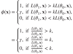
The Neyman-Pearson lemma is one of the ground-breaking results in statistics. It begins with the problem of testing a simple hypothesis against the simple hypothesis . The requirement of a size test with maximum power leads to the definition of a most powerful test.
The most powerful test is abbreviated as the MP test. We now state the lemma.
The test may be rewritten in the form of likelihood functions as
7.49
We will discuss some aspects of the Neyman-Pearson lemma before its applications. Some key points in this lemma are emphasized in the following:
a. Points are increased in the critical region until the size of the test reaches . To understand this, note that we consider the likelihood ratio and then rate the points of on the basis of the ratio of the explanation of under to the explanation under . Thus, the points with higher values of the likelihood ratio enjoy a better explanation under in comparison with .
b. The power of MP tests increases for corresponding increases in the test sizes.
d. The risk set defined in Equation 7.50 is a convex and compact set.
The Neyman-Pearson lemma will be illustrated through various examples now.
In the previous example, the value of under was less than under . Let us consider the same problem with roles reversed.
The reader may not be too comfortable with writing different programs, for the reason that may be lesser or greater than . Recall that the MPNormal function takes care of both scenarios. The next function takes care of this.
We will now move to the next type of hypotheses testing problem.
7.11 Uniformly Most Powerful Tests
The general one-sided hypothesis testing problem for a single real valued parameter is stated as:
Note that the hypotheses and are composite hypotheses. A definition of the size of a test for composite hypothesis is required.
We can now define the Uniformly Most Powerful Tests.
Let us first consider the problem of testing against . In this case the UMP test may be easily obtained. Towards this, fix a value and set up the Neyman-Pearson MP test for against . Then the MP test continues to be a UMP test if the test remains unaffected by the specific choice of .
We note that the UMP tests do not exist in general for one-sided testing problems. However, the UMP tests exist for a family of distribution satisfying a particular property. The mathematical property which is necessary for the existence of UMP tests is defined next.
A result due to Karlin and Rubin states that whenever there exists a statistic for which admits the MLR property, a UMP test can be constructed for the one-sided hypothesis.
7.12 Uniformly Most Powerful Unbiased Tests
The general hypotheses of interest is of the form: against . We will begin with an example.
It needs to be noted though that a UMP test for a simple hypothesis against the two-sided alternative exists for the uniform distribution, see Mukhopadhyay (2000). We will return to the problem of such hypotheses for the normal distribution. A condition needs to be relaxed for identifying meaningful tests and hence we consider the next definition.
Let denote the collection of all size unbiased tests. The next definition follows naturally.
The main reason for discussing the results in this fashion thus far is the integration of statistical concepts with R. It is believed that the reader is now convinced that the details of statistical theory can be understood using a software package. We now skip rest of the details, though illustrations are given, and simply leave it as an exercise for the reader to verify that the Student's -test is indeed a UMPU test. In fact, we need a host of other related and interesting concepts, such as similarity, to prove that the Student's -test is indeed a UMPU test. The details may be found in Lehmann and Romano (2005) and Srivastava and Srivastava (2009).
7.12.1 Tests for the Means: One- and Two-Sample t-Test
Assume that is a random sample from with both the parameters being unknown. Suppose we are interested in testing . The parameters and are respectively estimated using the sample mean and the sample standard deviation. The -test is then given by
7.59
which has a -distribution with degrees of freedom. The -test in R software may be found in the stats package whose constitution is given as
     t.test(x, y = NULL,
            alternative = c("two.sided", "less", "greater"),
            mu = 0, paired = FALSE, var.equal = FALSE,
            conf.level = 0.95, ...)
The following is clear from the above display:
1. The default function is a one-sample test with a two-sided alternative being tested for and 95% confidence interval as an output.
2. The user has the options of specifying the nature of alternatives, , and the confidence interval level.
In the above example we specified that is the mean of the parent height. However, a more appropriate test will be a direct comparison as to whether the height of the child is the same as the height of the parent.
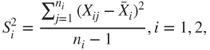
Let be a random sample from , and a random sample from , with unknown. Here, we assume that the variances are equal, though unknown. Suppose that we are interested to test the hypothesis against the hypothesis . The two-sample -test is then given by
7.60
which has a -distribution with degrees of freedom, with being the pooled standard deviation.
7.13 Likelihood Ratio Tests
Consider the generic testing problem vs . As earlier, it is assumed that a random sample of size is available.
The constant is to be determined from the size restriction:
The following examples deal with the construction of likelihood ratio tests.
The likelihood ratio tests are obtained for the normal distribution in the following subsections.
7.13.1 Normal Distribution: One-Sample Problems
In Section 7.11 we saw that UMP tests do not exist for many crucial types of hypothesis problems. As an example, for a random sample of size from , known, the UMP test does not exist for testing against . We will consider these types of problems in this subsection.
7.13.2 Normal Distribution: Two-Sample Problem for the Mean
As in the previous subsection, we will only consider the testing problem related to means. A very brief summary is given here.
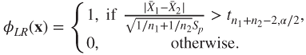
The general problem is described as follows. Let be a random sample from , and a random sample from . Assume that all the three parameters , and are unknown. For a specified level , the aim is to obtain the likelihood ratio test for testing against . Define the following quantities:
7.67
7.68
7.69
The size likelihood ratio test for against is given by
7.70
The next R function, LRNormal2Mean, with an illustration, gives the likelihood ratio test.
To the best of our knowledge, R does not have an implementation for the likelihood ratio test.
7.14 Behrens-Fisher Problem
In the two-sample problems for normal distributions considered earlier, the problem of testing against , when and are unknown and distinct, has not been considered. There has been a special reason for this. It has been proved by Linnik (1968) in this case that the UMPU test does not exist and there has been a lot of controversy surrounding the solutions proposed to date and it is even today an open problem.
The problem was first attempted by Behrens in 1929 and by Fisher in 1935. Kim and Cohen (1995) provide an excellent review of the solutions proposed by various statisticians. Schéffe (1943), Aspin (1948), Lindley (1965), Robinson (1976), and Welch (1938, 1947) are some of the important works in this direction.
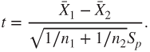
Suppose that we have observations from and observations from . As earlier, let denote the sample means, variances, and pooled variance. The Student's -test pivotal statistic with degrees of freedom is given by
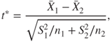
However, the Student's -test procedure makes the assumption of the variances being equal. Thus, the use of the -test is inappropriate here. An ad-hoc solution is the following. Compute by
and compare it with the critical value obtained from a variable with degrees of freedom. For a dataset from Kim and Cohen's review paper, an R program is given next.
A more satisfactory solution for the Behrens-Fisher problem is given by Welch and we will discuss his solution with an R program.
Compute the value of test statistic as the same given by . Define . Define
7.71
The Welch solution is to carry out the test by using the value and comparing it with a random variate with degrees of freedom. As may be expected, in general is not an integer. In such a case we round off the value to the nearest integer.
For more details related to the Behrens-Fisher problem, refer to the review article of Kim and Cohen.
7.15 Multiple Comparison Tests
Consider the following hypothesis:
7.72
Here, we have a set of hypotheses to be tested and this framework is popularly known as the multiple comparision test. Such hypotheses are very common in Experimental Designs, see Chapter 15. Suppose that , denotes the mean yield due to the -th treatment. In its general setup, the hypothesis says that none of the treatment means are significant. In case we fail to reject , the conclusion is indeed that none of the treatment means are significant and the analysis stops. However, if we reject the hypothesis , a host of questions then arise. In this case, the conclusion says that at least one treatment is significant and the interest is then to identify such a treatment. A slight variant of the problem is testing to some pre-specified level, which is generally known as the mean of the control treatment.
Let us begin with a naive approach. That is, we consider hypotheses instead of a single hypothesis and consider the problem of testing . Suppose each hypothesis is tested at level . A simple exploration shows the dire consequence of this naive approach. The forthcoming program will show that the probability of one or more false rejections increases drastically with .
That is, the Type I error grows very fast and with , we are almost certain of having committed the error. This motivates the next definition.
The goal of the multiple testing problem is to restrict the FWER to a pre-specified level :
7.74
In the next section we will focus on two simple, yet useful, procedures for the multiple testing problem.
7.15.1 Bonferroni's Method
The Bonferroni's method is a simple consequence of using the Bonferroni inequality. Let be the -value associated with hypothesis . Then reject the family of hypotheses if . It may be easily verified is this case that
An illustration will be provided for the example provided in R.
7.15.2 Holm's Method
Consider the ordered -values and let the associated hypotheses be . The Holm procedure is a stepdown procedure and is described below, adapted from page 351 of Lehmann and Romano (2005).
Step 1. If , accept and stop. If , reject and test the remaining hypotheses at level .
Step 2. If with , accept and stop. If and , reject and and test the remaining hypotheses at level .
Step 3. Continue the steps until .
For proof that the Holm's method meets the requirement , see Theorem 9.1.2 of Lehmann and Romano (2005). We will close the discussion with an example.
7.16 The EM Algorithm*
7.16.1 Introduction
The Expectation-Maximization Algorithm, more popularly known as the EM algorithm, is a very popular tool, not only among the statisticians, but also among the data miners. Wu and Kumar (2009) have selected the EM algorithm as one among the top ten useful algorithms for data miners. McLachlan and Krishnan (1998, 2008) give a rigorous mathematical introduction with a large number of illustrations of the EM algorithm. Little and Rubin (1987, 2002) is also one of the earliest books to give a detailed account of the algorithm. Dempster, Laird, and Rubin (1977) introduced the breakthrough EM algorithm and enhanced statistical methods which can accommodate missing data. This paper is also popularly referred to as the DLR paper. The introductory literature has so far been in reversed chronological order.
It is important to understand that the EM algorithm is not really an algorithm in the traditional usage of the technical word “algorithm”. It is a generic tool which gives rise to different statistical methods depending on the context of the application. Ripley in a reply to an R user has rightly explained this de facto as “The EM algorithm is not an algorithm for solving problems, rather an algorithm for creating statistical methods.”
In the context of handling missing data, Schafer (2000) has rightly said that “The key ideas behind EM and data augmentation are the same: to solve a difficult incomplete-data problem by repeatedly solving tractable complete-data problems.” Terry Speed (2008) has also said this about the EM algorithm: “I know many statisticians are deeply in love with the EM algorithm.”
“EMMIX” is probably one of the few softwares which implements the EM algorithm for the mixture of multivariate normal or - distribution.
7.16.2 The Algorithm
In general, the EM algorithm is stated in two steps: the E-step and the M-step. We will begin with a description as given in McLachlan and Krishnan (2008). Let be a random vector and be its observed value. The sample space of is denoted by . We will denote the pdf of by , where is the vector of unknown parameters.
To make use of the EM algorithm, we will always pretend that is incomplete in the sense that the experiment consists of some values which we treat as missing data. That is, we will assume that we have missing data in , and if this is augmented with , we will have the complete data in . Let denote the sample space of .
The pdf of the complete observation will be denoted by . Thus, under the assumption that is completely observed, the log-likelihood of is given by
7.75
Clearly, as the sample space of the 's is larger than the 's, we have a many-to-one mapping from to . Thus, the observed data can be written as the function . Hence, we have the relationship
Assume that we have an initial value as an estimate of in . Using the observed data and , we next specify the conditional probability distribution of . Since the complete data log-likelihood is not observable, we will replace it by its conditional expectation given and . This conditional expectation is the famous Q-function defined by
7.76
This is the famous E-step of the EM algorithm. In the M-step, we maximize to obtain such that
7.77
Thus, the EM algorithm can be summarized as below:
E-Stem: Calculate , where
7.78
M-Step: Select any value of , such that
7.79
The convergence criteria for the EM algorithm is that the difference should be approximately 0. This explanation of the EM algorithm in two steps can be found almost everywhere. However, we have found the five steps detail of the EM algorithm by Gupta and Chen (2011) to be more friendly and despite a repetition of the above content, we will state it here.
1. Set and obtain an initial estimate for as .
2. Assume that as the truth and using the observed data , completely specify the conditional probability distribution for the complete data .
3. Obtain the conditional expected log-likelihood Q-function:
4. Find , which maximizes .
5. Set and go to the first step.
We understand that the EM algorithm is best illustrated through applications.
7.16.3 Introductory Applications
We will consider problems which have been widely used illustrating the EM algorithm.
7.17 Further Reading
7.17.1 Early Classics
Fisher! In the 1920s, Sir R.A. Fisher wrote a series of ground-breaking papers on inference. Fisher (1925-1954) has given a first account on what should form the fundamentals of inference. Kendall and Stuart (1945–79) is one of the earliest and rigorous development of inference. Cramér's (1946) book is one of the landmarks for inference. Lehmann (1958) gave a detailed account related to testing of hypotheses. Rao (1965–73) is one of the all-time classics and goes beyond the “linear” indicated in its title. Wilks (1962), Zacks (1971), and Cox and Hinkley (1973) are some of the other rigorous books on statistical inference.
Let us now look at some of the earlier books which introduce the subject at an elementary level. Snedecor and Cochran (1937–89) may have been the first book on “Statistical Methods”. Mood, et al. (1950–74) is one of the earliest, elegant and elementary introduction to statistics. Hoel, et al. (1971), Hogg and Craig (1978), Hogg and Tanis (1977), and DeGroot and Schervish (2012), are also some of the best books written at their level.
In the Indian subcontinent, Das (1996) and Goon, et al. (1963) have written very useful texts.
7.17.2 Texts from the Last 30 Years
We do not intend to retain the chronological year of publication and jot down the texts which readily come to mind. As seen, chapter, Mukhopadhyay (2000), Rohatgi and Saleh (2000), and Casella and Berger (2000) have influenced this chapter a lot. Pawitan (2001) has been freely used for illustration of many concepts. Geisser and Johnson (2006) is a very compact work and will be useful to brush up on the details for an expert. Sen, et al. (2009) is a very concise course on the recent topics in inference. Wasserman (2004) is an advanced text which the reader will find useful for the modern development of the subject. Keener (2010), Dekking, et al. (2005), Liese and Miescke (2008), Knight (2000), Schervish (1995), and Shao (2003) are some of the finest written texts.
McLachlan and Krishnan (2008) is the first book to detail the EM algorithm. Huber and Ronchetti (2009) deals with the robustness of inference tools. As with the bibliography section of Chapter 5, we have again repeated a futile exercise.
7.18 Complements, Problems, and Programs
Problem 7.1 For different values of , obtain a plot of the curved normal family.
Problem 7.2 Italicize the -axis label in the expression part in Example 7.3.1.
Problem 7.3 Find a sufficient statistic for when .
Problem 7.4 Suppose follows a negative binomial distribution with parameters as defined in Equation (6.20). Assume that for obtaining failures, is noted as 10. Obtain the likelihood function plot and then graphically infer about the ML estimate of .
Problem 7.5 In a directory on a particular folder of a hard disk drive, there are files. Suppose that in a random selection of files, 9 are observed to be e-books. Under the assumption of a hypergeometric distribution, and by using the likelihood function approach, give the ML estimate of . Check Equation (6.30) if required to complete the R program.
Problem 7.6 For the two likelihood functions of the multinomial distribution in Examples 7.9.1 and 7.9.2, plot the likelihood function for obtaining the ML estimates.
Problem 7.7Section 7.6 makes use of the function optimize and mle to obtain the ML estimate. Will these techniques, return the ML estimate for the parameters in the previous two examples? If the technique fails, test across values of the parameters and data, what may be the reason behind it?
Problem 7.8 Using the Fishers score function technique, obtain the ML estimate in the previous three examples.
Problem 7.9 For the galton dataset from UsingR package, what will be the conclusion of the MP test that the height of the child is against , given that variance is known to be 1.7873.
Problem 7.10 If the variance is unknown in the previous example, carry out the likelihood-ratio test, see LRNormalMean_UV, and draw the conclusion at the level of significance.
Problem 7.11 In Section 7.12, it was mentioned that for a sample from a uniform distribution an UMP test exists for the hypothesis test problem of against . Obtain the UMP test and, if possible, an appropriate R program.
Problem 7.12 Assume that the variances for the two treatments of the Youden-Beale problem are unknown and there is no reasonable way they can be assumed to be equal. Use the two tests (R programs) developed in Section 7.14 in adhocBF and WelchBF to draw the right conclusions.
Problem 7.13 Carry out the multiple hypothesis testing problem, see glht function from the multcomp package, for the median polish regression model fitted in Section 4.5.2.
Problem 7.14 Interpret the R program in Example 7.10.2.
Problem 7.15 The -test used on the galton dataset is t.test(galton$child,mu=mean(galton$parent)). However, there is a “pairing” between the height of the child and the parent. Is the test t.test(galton$child,galton$parent,paired=TRUE) more appropriate?

 is a sufficient statistic for the family of distributions
  and a unique MLE of
  exists, then the MLE is a function of the sufficient statistic
  .
. is an MLE for
  and
and  is a one-to-one function of
  , then
  will be an MLE for
  .
.

 is independent of
  .
. exists
  .
. .
. .
. .
.
 . To understand this, note that we consider the likelihood ratio
  and then rate the points of
  on the basis of the ratio of the explanation of
  under
under  to the explanation under
  . Thus, the points with higher values of the likelihood ratio enjoy a better explanation under
  in comparison with
  .
. against
  is defined by7.50
 defined in Equation 7.50 is a convex and compact set.
 and 95% confidence interval as an output.
 , and the confidence interval level.
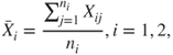
 , accept
  and stop. If
  , reject
  and test the remaining
  hypotheses at level
  .
. with
with  , accept
  and stop. If
  and
and 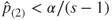 , reject
  and
and  and test the remaining
  hypotheses at level
  .
. .
. , where

 of
of  , such that

 and obtain an initial estimate for
  as
as  .
. as the truth and using the observed data
  , completely specify the conditional probability distribution
  for the complete data
  .
.
 , which maximizes
  .
. and go to the first step.
 , obtain a plot of the curved normal family.
 -axis label in the
  when
when  .
. follows a negative binomial distribution with parameters as defined in Equation (6.20). Assume that for obtaining
  failures,
  is noted as 10. Obtain the likelihood function plot and then graphically infer about the ML estimate of
  .
. files. Suppose that in a random selection of
  files, 9 are observed to be e-books. Under the assumption of a hypergeometric distribution, and by using the likelihood function approach, give the ML estimate of
  . Check Equation (6.30) if required to complete the R program.
 against
  , given that variance is known to be 1.7873.
 level of significance.
 against
  . Obtain the UMP test and, if possible, an appropriate R program.
 -test used on the