In many real-world problems, data is seldom univariate. We have more than one variable, which needs a good understanding of the underlying uncertain phenomenons. Thus, we need a set of tools to handle this type of data, and this is provided by Multivariate Statistical Analysis (MSA), a branch of the subject. We saw in the previous chapters on regression, that multiple regressors explain the regressand. Sometimes experiments may need a deeper study of the covariates themselve. In particular, we are now concerned with a random vector, the characteristics of which form the crux of this and the next chapter.
In Section 14.2 we look at graphical plots, which give a deeper insight into the structure of the dataset. The core concepts of MSA are introduced in Section 14.3. Sections 14.4 and 14.5 deal with the inference problem related to the mean vectors of multivariate data, whereas inference related with the variance-covariance matrix are performed in Sections 14.7 and 14.8. Multivariate Analysis of Variance, abbreviated as MANOVA, tools are introduced and illustrated in Section 14.6 and some tests for independence of sub-vectors are addressed in Section 14.9. Advanced topics of multivariate statistical analysis are carried over to the next chapter.
14.2 Graphical Plots for Multivariate Data
In Chapter 12 we saw the use of scatter plots and pairs (matrix of scatter plots). A slight modification of the matrix of a scatter plot is considered here, which gives more insight into the multivariate aspect of the dataset. Multi-dimensional data can be still visualized in two dimensions and a particularly effective technique provided by Chernoff faces is detailed. We will begin with a multivariate dataset.
Chernoff (1973) gave a very innovative technique to visualize multivariate data, which considers each variate as some dimension of the human face, say nose, ears, smile, cheeks, etc. Interpretation of three-dimensional plots itself is difficult, even if we were to deploy features such as rotation of the plots. Certainly, visualization in more than three dimensions is not possible. Thus, the Chernoff technique of visualizing the multivariate data through faces is very helpful and such a plot is of course well known as the Chernoff faces. We deploy this method here using the graphical function faces from the R package aplpack.
Chernoff faces gives one facet of data visualization of multivariate data. There are many other similar techniques, though we will not dwell more on them. In the next Section 14.3 we consider more basic aspects of the multivariate and define the multivariate normal distribution in more detail.
14.3 Definitions, Notations, and Summary Statistics for Multivariate Data
14.3.1 Definitions and Data Visualization
We will denote a -random vector by , and its replicates by . The random vector of the replicate is denoted as . The mean vector and variance-covariance matrix of X are respectively denoted as
14.1
14.2
14.3
Note that the matrix is a symmetric matrix, that is, .
Sometimes, we may also be interested in the correlation matrix defined by
Each correlation coefficient will be a number between –1 and +1, that is, .
The -dimensional normal density will be denoted by . The case of refers to the bivariate normal random distribution. For bivariate normal random variables with a zero-mean vector and a couple of positive and negative correlations, we obtain the probability density plots.
We now describe some standard methods of estimation of the mean vector and the variance-covariance matrix. Define
14.5
14.6
Result 4.11 of Johnson and Wichern (2006) shows that the estimators and are respectively MLE's of their parameters.
14.3.2 Early Outlier Detection
An important concept for analysis of multivariate data is given by the Mahalanobis distance.
Thus, for each vector , the Mahalanobis distance may be computed and any unusually large value may then be marked as an outlier. The Mahalanobis distance is also called the generalized squared distance.
It is a familiar story that outliers, as in univariate cases, need to be addressed as early as possible. Graphical methods become a bit difficult if the number of variables is more than three. Johnson and Wichern (2006) suggest we should obtain the standardized values of the observations with respect to each variable, and they also recommend looking at the matrix of scatter plots. The four steps listed by them are:
Obtain the dot plot for each variable.
Obtain the matrix of scatter plots.
Obtain the standardized scores for each variable, , for , and . Check for large and small values of these scores.
Obtain the generalized squared distances . Check for large distances.
A dot plot is also known as a Cleveland dot plot and it is set up using the dotchart function, which in turn is a substitute to the bar plot. In this plot, a dot is used to represent the magnitude of the observation along the -axis with the observation number on the -axis.
We have seen some interesting graphical plots for the multivariate data. The multivariate normal distribution has also been introduced here, along with a few of its properties. We will next consider some testing problems for multivariate normal distribution.
14.4 Testing for Mean Vectors : One Sample
Suppose that we have random vector samples from a multivariate normal distribution, say . In Chapter 7, we saw testing problems for the univariate normal distribution. If the variance-covariance matrix is known to be a diagonal matrix, that is components are uncorrelated random variables, we can revert back to the methods discussed there. However, this is not generally the case for multivariate distributions and they need specialized methods for testing hypothesis problems.
For the problem of testing against , we consider two cases here: (i) is known, and (ii) is unknown. Suppose that we have samples of random vectors from , which we will denote as . The sample of random vectors is the same as saying that we have iid random vectors.
14.4.1 Testing for Mean Vector with Known Variance-Covariance Matrix
If the variance-covariance matrix is known, the test statistic is a multivariate extension of the -statistic, and is given by
14.8
Under the hypothesis , the test statistic is distributed as a chi-square variate with degrees of freedom, and a random variable. The computations are fairly easy and we do that in the next example.
14.4.2 Testing for Mean Vectors with Unknown Variance-Covariance Matrix
It turns out that in many practical settings, the variance-covariance matrix is unknown. Therefore, we need to extend the test procedure for this important case. The Hotelling's -statistic is given by
14.9
where is the sampling covariance matrix. Under the hypothesis , the test statistic is distributed as Hotellings' distribution with and degrees of freedom.
The Hotellings' can be converted to an -statistics using the transformation:
14.10
An R function for calculating the test statistic is available in the ICSNP package. The test function HotellingsT2 implements the -test by comparing if the mean of a normal vector equals some specified null vector. We can easily carry out the -test for the above example.
It is known that the likelihood-ratio tests are very generic methods for testing hypothesis problems. The likelihood-ratio test of against is given by
14.11
It is further known from the general theory of the likelihood ratios that the above-mentioned test statistics follow a chi-square random variate. Yes, the computations are not trivial for the -test based on the likelihood-ratio test, and hence the ICSNP package will be used to bail us out of this scenario. The illustration is continued with the previous data-set.
The problem of testing against will be considered for the two-sample problem in Section 14.5.
14.5 Testing for Mean Vectors : Two-Samples
Consider the case of random vector samples from two plausible populations, and . Such scenarios are very likely if new machinery and a population labeled 1 refers to samples obtained under the new machinery and that labeled 2 refers to the samples under older machinery. As the comparison of the mean vectors become sensible only if the covariance matrices are equal, we assume that the covariance matrices are equal, but not known. That is, , with unknown.
Suppose that we have samples from the two populations as , , and , . The hypothesis of interest is to test against . The estimates of the mean vectors from each of the populations is given by .
We will first define the matrices of sum squares and cross-products as below:
The test statistic , under the hypothesis , is distributed as Hotelling's distribution with parameters and . We list below some important properties of the Hotelling's statistic:
1. Hotelling's distribution is skewed.
2. For a two-sided alternative hypothesis, the critical-region is one-tailed.
3. A necessary condition for the inverse of the pooled covariance matrix to exist is that the .
4. A straightforward, not necessarily simple, transformation of the Hotelling's statistic gives us an -statistic.
As in the previous section, we may also use the likelihood-ratio tests, which lead to an appropriate -test, for large of course, see Rencher (2002) or Johnson and Wichern (2006). In the next illustrative example, we obtain the Hotelling's test statistics, the associated -statistic, and the likelihood-ratio test.
14.6 Multivariate Analysis of Variance
The ANOVA deals with testing of -means being equal in the univariate case. A host of ANOVA techniques was seen in Chapter 13. For the multivariate case, we have the generalization multivariate analysis of variance, more commonly simply known as MANOVA. The data structure can be easily displayed in tabular form, and we adapt the notation from Rencher (2002).
Suppose we want to test for equality of mean of -vector samples. Let denote observation from population , . We assume that . The observation model is specified by
14.16
Here , and is the mean effect in the population. The hypothesis of interest is given by . To test the hypothesis , we need to define, as usual, the “between” and “within” sum of squares matrices, denoted by and respectively:
Let and respectively denote the rank of and . There are four different statistics to test for and they are now explained in some detail.
14.6.1 Wilks Test Statistic
The Wilks test statistic for is given by
14.19
In the above expression, denotes the determinant of the matrix. The multivariate literature refers to as Wilks' . The test statistic can be equivalently expressed in terms of the eigenvalues of , where is the rank of , and is given by
14.20
The Wilks' takes values in the interval . Thus, the test procedure is to reject if . These ideas and concepts are next illustrated using the well-known root-stack dataset.
14.6.2 Roy's Test
It is beyond the scope of the current work to clearly underpin the statistical motivation of Roy's test. An elegant description of the Roy's test can be found in Section 6.1.4 of Rencher (2002). We now give a watered-down version of Roy's test. Let denote the largest eigenvalue of the matrix . The Roy's largest root test is given by
The test procedure is to reject if . In R, we carry out the Pillai's method as below.
> summary(root.manova, test = "Pillai")
          Df Pillai approx F num Df den Df Pr(>F)
rs         5   1.30     4.07     20    168  2e-07 ***
Residuals 42
---
Signif. codes:  0 '***' 0.001 '**' 0.01 '*' 0.05 '.' 0.1 ' ' 1
The Pillai's test statistic confirms the findings of the Wilks's and Roy's test that the mean vector for the six strata are significantly different. Finally, we look at the fourth test for testing the hypothesis , that the strata mean vectors are equal to the Lawley-Hotelling test statistic.
The test procedure is to reject the hypothesis for large values of . This is illustrated in R.
> summary(root.manova, test = "Hotelling")
          Df Hotelling-Lawley approx F num Df den Df  Pr(>F)
rs         5             2.92     5.48     20    150 2.6e-10 ***
Residuals 42
---
Signif. codes:  0 '***' 0.001 '**' 0.01 '*' 0.05 '.' 0.1 ' ' 1
Thus, it is concluded that all the four statistical tests lead to the same conclusion, that the mean vector for the six strata are different. From a theoretical point of view, there is no reason to prefer one of the four methods over the others. A general advice is to use all the four methods. Consider one more example before closing the MANOVA section.
We will next look at testing hypotheses problems related to the variance-covariance matrices.
14.7 Testing for Variance-Covariance Matrix: One Sample
In MSA, the covariance matrix plays the role of the scale parameter. We thus naturally encounter the problem of testing . Let us begin with the testing problems of covariance matrix in the one sample case.
Let denote the sample covariance matrix of . Define . The likelihood ratio test statistic for the hypothesis is given by
where is the degrees of freedom of , is the natural logarithm (base ), and tr is the trace, sum of diagonal matrix, of a matrix. For large values, is approximately distributed as a - random variable with degrees of freedom. For moderate-sized samples, Rencher (2002) recommends the use of the following modification:
The test procedure is to reject the hypothesis if the values of or are greater than . Both the test statistics and are computed in the next example.
14.7.1 Testing for Sphericity
The problem of testing if the components of a random vector are independent is equivalent to the problem of testing , where is the identity matrix. We would like to caution the reader to always keep in mind the counter-example of Section 14.3. The hypothesis is that we are testing equivalent tests if all the correlations among the component are equal to zero, that is, it examines if the components are independent.
Note that if the hypothesis holds true, the ellipsoid becomes , which is the equation of a sphere. Here, is some non-negative constant, that is, . Hence, the problem of a test for independence of the components is also known as tests of sphericity.
The log-likelihood ratio test for is given by
which on further evaluation leads to
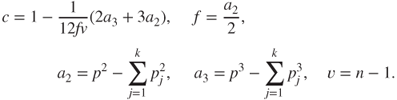
where . The test statistic can be restated in terms of the eigenvalues as
where is the degrees of freedom of . The statistic , under the hypothesis , has a distribution with degrees of freedom. The test procedure is to reject the hypothesis if .
14.8 Testing for Variance-Covariance Matrix: -Samples
Consider the case when we have samples from -populations, that is, , for . For the sample, we have a sample of size . The hypothesis of interest here is . Also, define the following:
: the sample covariance matrix of the population;
: the degrees of freedom associated with the estimated covariance matrix .
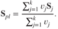
Technically, we need to have for ensuring that the estimated covariance matrices are non-singular. Define the pooled sample covariance matrix by
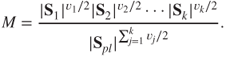
The test statistic for the hypothesis is then given by the following:
14.28
The range of values for is between 0 and 1, with values closer to 1 favoring the hypothesis , and values closer to 0 leading to its rejection. This can be easily seen by rewriting the expression of as
The hypothesis may be tested using the exact M-test with , see page 258 of Rencher (2002).
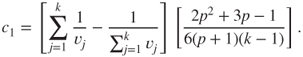
To test the hypothesis , we may also use the Box's and - approximations for the probability distribution of . Towards this, we will first define as follows:
is distributed as a random variable with degrees of freedom.
The steps for obtaining the -approximation may appear cumbersome, but its benefits are also equally rewarding. As with the approximation, we will first define the required quantities. Define as a function of by
In both cases, the approximation follows the distribution, and the test procedure is to reject the hypothesis if .
14.9 Testing for Independence of Sub-vectors
The test of sphericity addresses the problem of testing if all the covariates are independent or not. A very likely practical problem could be that we may know beforehand that certainly not all the components are independent. However, we may also have knowledge that though the first three components and the next four components are related, it may be the case that the set of the first three components are independent of the set of the next four components. We would thus like to have some statistical tests to help us prove if our hypothesis is true or not. In fact, we need methods to help us test any combination of vectors as independent or not, and the methods in this section exactly help us to accomplish this.
Consider the -dimensional random vector . Suppose that we are interested to find if the sub-vectors are a mutually independent sets of sub-vectors. The notation needs a bit of explanation. If , we are testing if all the components are independent. We denote for the number of elements in the sub-vector , and we require that . Note that denotes a partitioning of and not a random sample of size of .
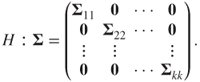
Let denote the covariance matrix between the sub-vectors and , . The hypothesis for independence of the sub-vectors can then be stated symbolically as , , and in matrix notation as below:
14.36
Let us denote the partition of estimated covariance matrix by the following:
In the next chapter on MSA, we will consider some of the more advanced topics, which are more useful in an applied context.
14.10 Further Reading
Anderson (1953, 1984, and 2003) is the first comprehensive and benchmark book in this area of statistics. Rencher (2002), Johnson and Wichern (2007), Hair, et al. (2010), Hardle and Simar (2007), and Izenman (2008) are some of the modern accounts of multivariate statistical analysis. Everitt (2005) has handled the associated computations through R and S-Plus. However, as Everitt (2005) and Everitt and Hothorn (2011) are dwelling more in advanced methods of MSA, we believe that the reader can benefit from the coverage given in this and the next chapter.
14.11 Complements, Problems, and Programs
Problem 14.1 The iris data has been introduced in AD2. Obtain the matrix of scatter plots for (i) the overall dataset (removing the Species), and (ii) three subsets according to the Species. Obtain the average of the four characteristics by the Species group and using the faces function from the aplpack package, plot the Chernoff faces. Do the Chernoff faces offer enough insight to identify the group?
Problem 14.2 For the board stiffness data discussed in Example 14.3.3, obtain the covariance matrix and then using the cov2cor function, obtain the correlation matrix.
Problem 14.3 The Mahalanobis distance given in Equation 14.7 is easily obtained in R using the mahalanobis function. Using this function, obtain the distance of the observations from the entire dataset for the board stiffness dataset and investigate for presence of outliers. Repeat the exercise for the presence of outliers in the iris dataset too.
Problem 14.4 Using the HotellingsT2 function from the ICSNP package, test whether average sepal and petal length and width for setosa species equals [5.936 2.770 4.260 1.326] in the iris dataset.
Problem 14.5 Using the HotellingsT2 function from the ICSNP package, test whether average sepal and petal length and width for setosa species equals that of versicolor in the iris dataset.
Problem 14.6 Run the example code of the function HotellingsT2, that is run example(HotellingsT2), and explore the options available with this function.
Problem 14.7 Carry out the MANOVA analysis for the iris datasets, where the hypothesis problem is that the mean of the multivariate vector of the four variables are equal across the three types of species.
Problem 14.8 Using base matrix tools of R, create a function which returns the value of Roy's test statistic given in Equation 14.21.
Problem 14.9 Repeat the above exercise for the Pillai and Lawley-Hotelling tests respectively given in Equations 14.22 and 14.23.
Problem 14.10 For the iris dataset, test the hypothesis . Repeat the exercise for the stack loss problem too.
Problem 14.11 Test whether the Sepal and Petal characteristics are independent of each other in the iris dataset.


 , for
, for  , and
, and  . Check for large and small values of these scores.
 . Check for large distances.
 distribution is skewed.
 .
. -statistic.
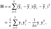


 -Samples
 : the sample covariance matrix of the
  population;
 : the degrees of freedom associated with the estimated covariance matrix
  .
.


 given in Equation 14.7 is easily obtained in R using the
  . Repeat the exercise for the stack loss problem too.