
Chapter 6. Basic Pathfinding and Waypoints
Many different types of pathfinding problems exist. Unfortunately, no one solution is appropriate to every type of pathfinding problem. The solution depends on the specifics of the pathfinding requirements for any given game. For example, is the destination moving or stationary? Are obstacles present? If so, are the obstacles moving? What is the terrain like? Is the shortest solution always the best solution? A longer path along a road might be quicker than a shorter path over hills or swampland. It’s also possible that a pathfinding problem might not even require reaching a specific destination. Perhaps you just want a game character to move around or explore the game environment intelligently. Because there are so many types of pathfinding problems, it wouldn’t be appropriate to select just one solution. The A∗ algorithm, for example, although an ideal solution for many pathfinding problems, isn’t appropriate for every situation. This chapter explores some of the techniques you can use for situations in which the A∗ algorithm might not be the best solution. We’ll cover the venerable A∗ algorithm in Chapter 7.
Basic Pathfinding
At its most basic level, pathfinding is simply the process of moving the position of a game character from its initial location to a desired destination. This is essentially the same principle we used in the basic chasing algorithm we showed you in Chapter 2. Example 6-1 shows how you can use this algorithm for basic pathfinding.
if(positionX > destinationX)
positionX--;
else if(positionX < destinationX)
positionX++;
if(positionY > destinationY)
positionY--;
else if(positionY < destinationY)
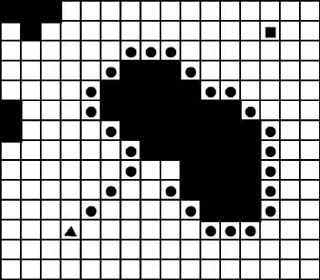
positionY++;In this example, the position of the game character is specified using the positionX and positionY variables. Each time this code is executed, the positionX and positionY coordinates are either increased or decreased so that the game character’s position moves closer to the destinationX and destinationY coordinates. This is a simple and fast solution to a basic pathfinding problem. However, like its chasing algorithm counterpart from Chapter 2, it does have some limitations. This method produces an unnatural-looking path to the destination. The game character moves diagonally toward the goal until it reaches the point where it is on the same x- or y-axis as the destination position. It then moves in a straight horizontal or vertical path until it reaches its destination. Figure 6-1 illustrates how this looks.
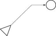
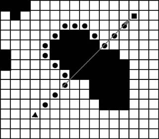
As Figure 6-1 shows, the game character (the triangle) follows a rather unnatural path to the destination (the circle). A better approach would be to move in a more natural line-of-sight path. As with the line-of-sight chase function we showed you in Chapter 2, you can accomplish this by using the Bresenham line algorithm. Figure 6-2 illustrates how a line-of-sight path using the Bresenham line algorithm appears relative to the basic pathfinding algorithm shown in Example 6-1.
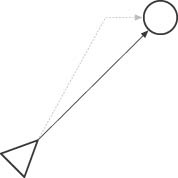
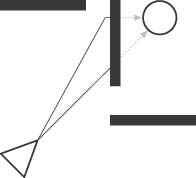
As you can see in Figure 6-2, the line-of-sight approach produces a more natural-looking path. Although the line-of-sight method does have some advantages, both of the previous methods produce accurate results for basic pathfinding. They are both simple and relatively fast, so you should use them whenever possible. However, the two previous methods aren’t practical in many scenarios. For example, having obstacles in the game environment, such as in Figure 6-3, can require some additional considerations.
Random Movement Obstacle Avoidance
Random movement can be a simple and effective method of obstacle avoidance. This works particularly well in an environment with relatively few obstacles. A game environment with sparsely placed trees, such as the one shown in Figure 6-4, is a good candidate for the random movement technique.
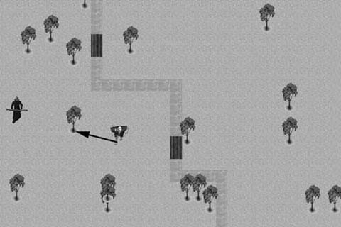
As Figure 6-4 shows, the player is not in the troll’s line of sight. However, because so few obstacles are in the environment, when you simply move the troll in almost any direction the player will enter the troll’s line of sight. In this scenario, a CPU-intensive pathfinding algorithm would be overkill. On the other hand, if the game environment were composed of many rooms with small doorways between each room, the random movement method probably wouldn’t be an ideal solution. Example 6-2 shows the basic algorithm used for random movement obstacle avoidance.
   if Player In Line of Sight
      {
          Follow Straight Path to Player
      }
   else
      {
          Move in Random Direction
      }
computer-controlled character is moved in a random direction. Because so few obstacles are in the scene, it’s likely that the player will be in the line of sight the next time through the game loop.
Tracing Around Obstacles
Tracing around obstacles is another relatively simple method of obstacle avoidance. This method can be effective when attempting to find a path around large obstacles, such as a mountain range in a strategy or role-playing game. With this method, the computer-controlled character follows a simple pathfinding algorithm in an attempt to reach its goal. It continues along its path until it reaches an obstacle. At that point it switches to a tracing state. In the tracing state it follows the edge of the obstacle in an attempt to work its way around it. Figure 6-5 illustrates how a hypothetical computer-controlled character, shown as a triangle, would trace a path around an obstacle to get to its goal, shown as a square.
Besides showing a path around the obstacle, Figure 6-5 also shows one of the problems with tracing: deciding when to stop tracing. As Figure 6-5 shows, the outskirts of the obstacle were traced, but the tracing went too far. In fact, it’s almost back to the starting point. We need a way to determine when we should switch from the tracing state back to a simple pathfinding state. One way of accomplishing this is to calculate a line from the point the tracing starts to the desired destination. The computer-controlled character will continue in the tracing state until that line is crossed, at which point it reverts to the simple pathfinding state. This is shown in Figure 6-6.
Tracing the outskirts of the obstacle until the line connecting the starting point and desired destination is crossed ensures that the path doesn’t loop back to the starting point. If another obstacle is encountered after switching back to the simple pathfinding state, it once again goes into the tracing state. This continues until the destination is reached.
Another method is to incorporate a line-of-sight algorithm with the previous tracing method. Basically, at each step along the way, we utilize a line-of-sight algorithm to determine if a straight line-of-sight path can be followed to reach the destination. This method is illustrated in Figure 6-7.

As Figure 6-7 shows, we follow the outskirts of the obstacle, but at each step we check to see if the destination is in the computer-controlled character’s line of sight. If so, we switch from a tracing state to a line-of-sight pathfinding state.
Breadcrumb Pathfinding
Breadcrumb pathfinding can make computer-controlled characters seem very intelligent because the player is unknowingly creating the path for the computer-controlled character. Each time the player takes a step, he unknowingly leaves an invisible marker, or breadcrumb, on the game world. When a game character comes in contact with a breadcrumb, the breadcrumb simply begins following the trail. The game character will follow in the footsteps of the player until the player is reached. The complexity of the path and the number of obstacles in the way are irrelevant. The player already has created the path, so no serious calculations are necessary.
The breadcrumb method also is an effective and efficient way to move groups of computer-controlled characters. Instead of having each member of a group use an expensive and time-consuming pathfinding algorithm, you can simply have each member follow the leader’s breadcrumbs.
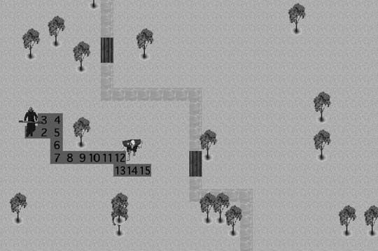
Figure 6-8 shows how each step the player takes is marked with an integer value. In this case, a maximum of 15 steps are recorded. In a real game, the number of breadcrumbs dropped will depend on the particular game and how smart you want the game-controlled characters to appear. In this example, a troll randomly moves about the tile-based environment until it detects a breadcrumb on an adjacent location.
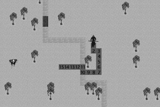
Of course, in a real game, the player never sees the breadcrumb trail. It’s there exclusively for the game AI. Example 6-3 shows the class we use to track the data associated with each game character.
#define   kMaxTrailLength   15
class	   ai_Entity
{
       public:
       int   row;
       int   col;
       int   type;
       int   state;
       int   trailRow[kMaxTrailLength];
       int   trailCol[kMaxTrailLength];
       ai_Entity();
       ~ai_Entity();
};
The initial #define statement sets the maximum number of player steps to track. We then use the kMaxTrailLength constant to define the bounds for the trailRow and trailCol arrays. The trailRow and trailCol arrays store the row and column coordinates of the previous 15 steps taken by the player.
As Example 6-4 shows, we begin by setting each element of the trailRow and trailCol arrays to a value of −1. We use −1 because it’s a value outside of the coordinate system we are using for this tile-based demo. When the demo first starts, the player hasn’t taken any steps, so we need a way to recognize that some of the elements in the trailRow and trailCol arrays haven’t been set yet.
int   i;
for (i=0;i<kMaxTrailLength;i++)
   {
      trailRow[i]=-1;
      trailCol[i]=-1;
   }
As you can see in Example 6-4, we traverse the entire trailRow and trailCol arrays, setting each value to −1. We are now ready to start recording the actual footsteps. The most logical place to do this is in the function that changes the player’s position. Here we’ll use the KeyDown function. This is where the demo checks the four direction keys and then changes the player’s position if a key-down event is detected. The KeyDown function is shown in Example 6-5.
void ai_World::KeyDown(int key)
{
     int   i;
   if (key==kUpKey)
       for (i=0;i<kMaxEntities;i++)
          if (entityList[i].state==kPlayer)
              if (entityList[i].row>0)
                 {
                    entityList[i].row--;
                    DropBreadCrumb();
                 }
   if (key==kDownKey)
       for (i=0;i<kMaxEntities;i++)
          if (entityList[i].state==kPlayer)
              if (entityList[i].row<(kMaxRows-1))
                 {
                    entityList[i].row++;
                    DropBreadCrumb();
                 }
   if (key==kLeftKey)
       for (i=0;i<kMaxEntities;i++)
           if (entityList[i].state==kPlayer)
               if (entityList[i].col>0)
                  {
                     entityList[i].col--;
                     DropBreadCrumb();
                  }
   if (key==kRightKey)
       for (i=0;i<kMaxEntities;i++)
          if (entityList[i].state==kPlayer)
             if (entityList[i].col<(kMaxCols-1))
                {
                   entityList[i].col++;
                   DropBreadCrumb();
                }
}
The KeyDown function shown in Example 6-5 determines if the player has pressed any of the four direction keys. If so, it traverses the entityList array to search for a character being controlled by the player. If it finds one, it makes sure the new desired position is within the bounds of the tile world. If the desired position is legitimate, the position is updated. The next step is to actually record the position by calling the function DropBreadCrumb. The DropBreadCrumb function is shown in Example 6-6.
void ai_World::DropBreadCrumb(void)
{
    int   i;
    for (i=kMaxTrailLength-1;i>0;i--)
        {
           entityList[0].trailRow[i]=entityList[0].trailRow[i-1];
           entityList[0].trailCol[i]=entityList[0].trailCol[i-1];
        }
    entityList[0].trailRow[0]=entityList[0].row;
    entityList[0].trailCol[0]=entityList[0].col;
}
The DropBreadCrumb function adds the current player position to the trailRow and trailCol arrays. These arrays maintain a list of the most recent player positions. In this case, the constant kMaxTrailLength sets the number of positions that will be tracked. The longer the trail, the more likely a computer-controlled character will discover it and pathfind its way to the player.
The DropBreadCrumb function begins by dropping the oldest position in the trailRow and trailCol arrays. We are tracking only kMaxTrailLength positions, so each time we add a new position we must drop the oldest one. We do this with the initial for loop. In effect, this loop shifts all the positions in the array. It deletes the oldest position and makes the first array element available for the current player position. Next, we store the player’s current position in the first element of the trailRow and trailCol arrays.
The next step is to actually make the computer-controlled character detect and follow the breadcrumb trail that the player is leaving. The demo begins by having the computer-controlled troll move randomly about the tiled environment. Figure 6-9 illustrates how the troll moves about the tiled environment in any one of eight possible directions.
Example 6-7 goes on to show how the troll detects and follows the breadcrumb trail.
for (i=0;i<kMaxEntities;i++)
    {
       r=entityList[i].row;
       c=entityList[i].col;
       foundCrumb=-1;
       for (j=0;j<kMaxTrailLength;j++)
       {
          if ((r==entityList[0].trailRow[j]) &&
               (c==entityList[0].trailCol[j]))
             {
                foundCrumb=j;
                break;
             }
          if ((r-1==entityList[0].trailRow[j]) &&
               (c-1==entityList[0].trailCol[j]))
             {
                foundCrumb=j;
                break;
             }
         if ((r-1==entityList[0].trailRow[j]) &&
              (c==entityList[0].trailCol[j]))
            {
               foundCrumb=j;
               break;
            }
         if ((r-1==entityList[0].trailRow[j]) &&
              (c+1==entityList[0].trailCol[j]))
            {
               foundCrumb=j;
               break;
            }
         if ((r==entityList[0].trailRow[j]) &&
              (c-1==entityList[0].trailCol[j]))
            {
               foundCrumb=j;
               break;
            }
         if ((r==entityList[0].trailRow[j]) &&
              (c+1==entityList[0].trailCol[j]))
            {
               foundCrumb=j;
               break;
            }
         if ((r+1==entityList[0].trailRow[j]) &&
              (c-1==entityList[0].trailCol[j]))
            {
               foundCrumb=j;
               break;
            }
         if ((r+1==entityList[0].trailRow[j]) &&
              (c==entityList[0].trailCol[j]))
            {
               foundCrumb=j;
               break;
            }
         if ((r+1==entityList[0].trailRow[j]) &&
              (c+1==entityList[0].trailCol[j]))
            {
               foundCrumb=j;
               break;
            }
      }
      if (foundCrumb>=0)
          {
             entityList[i].row=entityList[0].trailRow[foundCrumb];
             entityList[i].col=entityList[0].trailCol[foundCrumb];
          }
      else
         {
            entityList[i].row=entityList[i].row+Rnd(0,2)-1;
            entityList[i].col=entityList[i].col+Rnd(0,2)-1;
         }
      if (entityList[i].row<0)
         entityList[i].row=0;
      if (entityList[i].col<0)
         entityList[i].col=0;
      if (entityList[i].row>=kMaxRows)
         entityList[i].row=kMaxRows-1;
      if (entityList[i].col>=kMaxCols)
         entityList[i].col=kMaxCols-1;
   }
the trailRow and trailCol arrays are ordered from the most recent player position to the oldest player position. Starting the search from the most recent player position also ensures that the troll will follow the breadcrumbs to, rather than away from, the player. It’s quite probable that the troll will first detect a breadcrumb somewhere in the middle of the trailRow and trailCol arrays. We want to make sure the troll follows the breadcrumbs to the player.
Once the for loop is finished executing, we check whether a breadcrumb has been found. The foundCrumb variable stores the array index of the breadcrumb found. If no breadcrumb is found, it contains its initial value of −1. If foundCrumb is greater than or equal to 0, we set the troll’s position to the value stored at array index foundCrumb in the trailRow and trailCol arrays. Doing this each time the troll’s position needs to be updated results in the troll following a trail to the player’s position.
If foundCrumb is equal to a value of −1 when we exit the for loop, we know that no breadcrumbs were found. In this case, we simply select a random direction in which to move. Hopefully, this random move will put the troll adjacent to a breadcrumb which can be detected and followed the next time the troll’s position needs to be updated.
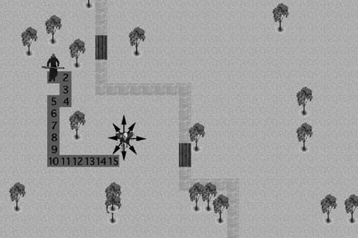
There is another benefit to storing the most recent player positions in the lower trailRow and trailCol array elements. It is not unusual for a player to backtrack or to move in such a way that his path overlaps with or is adjacent to a previous location. This is illustrated in Figure 6-10.
In this case, the troll isn’t going to follow the exact footsteps of the player. In fact, doing so would be rather unnatural. It would probably be obvious to the player that the troll was simply moving in the player’s footsteps rather than finding its way to the player in an intelligent way. In this case, however, the troll will always look for the adjacent tile containing the most recent breadcrumb. The end result is that the troll will skip over breadcrumbs whenever possible. For example, in Figure 6-10, the troll would follow array elements {12,11,10,9,8,7,6,2} as it moves to the player’s position.
Path Following
Pathfinding is often thought of solely as a problem of moving from a starting point to a desired destination. Many times, however, it is necessary to move computer-controlled characters in a game environment in a realistic way even though they might not have an ultimate destination. For example, a car-racing game would require the computer-controlled cars to navigate a roadway. Likewise, a strategy or role-playing game might require troops to patrol the roads between towns. Like all pathfinding problems, the solution depends on the type of game environment. In a car-racing game the environment probably would be of a continuous nature. In this case the movement probably would be less rigid. You would want the cars to stay on the road, but in some circumstances that might not be possible. If a car tries to make a turn at an extremely high rate of speed, it likely would run off the road. It could then attempt to slow down and steer back in the direction of the road.
You can use a more rigid approach in a tile-based game environment. You can think of this as more of a containment problem. In this scenario the game character is confined to a certain terrain element, such as a road. Figure 6-11 shows an example of this.
In Figure 6-11, all the terrain elements labeled as 2s are considered to be the road. The terrain elements labeled as 1s are considered to be out of bounds. So, this becomes a matter of containing the computer-controlled troll to the road area of the terrain. However, we don’t want the troll to simply move randomly on the road. The result would look unnatural. We want the troll to appear as though it’s walking along the road. As you’ll notice, the road is more than one tile thick, so this isn’t just a matter of looking for the next adjacent tile containing a 2 and then moving there. We need to analyze the surrounding terrain and decide on the best move. A tile-based environment typically offers eight possible directions when moving. We examine all eight directions and then eliminate those that are not part of the road. The problem then becomes one of deciding which of the remaining directions to take. Example 6-8 shows how we begin to analyze the surrounding terrain.
int   r;
int   c;
int   terrainAnalysis[9];
r=entityList[i].row;
c=entityList[i].col;
terrainAnalysis[1]=terrain[r-1][c-1];
terrainAnalysis[2]=terrain[r-1][c];
terrainAnalysis[3]=terrain[r-1][c+1];
terrainAnalysis[4]=terrain[r][c+1];
terrainAnalysis[5]=terrain[r+1][c+1];
terrainAnalysis[6]=terrain[r+1][c];
terrainAnalysis[7]=terrain[r+1][c-1];
terrainAnalysis[8]=terrain[r][c-1];
for (j=1;j<=8;j++)
   if (terrainAnalysis[j]==1)
      terrainAnalysis[j]=0;
   else
      terrainAnalysis[j]=10;
We begin defining the terrainAnalysis array. This is where we will store the terrain values from the eight tiles adjacent to the computer-controlled troll. We do this by offsetting the current row and column positions of the troll. After the eight values are stored, we enter a for loop which determines if each value is part of the road. If it’s not part of the road, the corresponding terrainAnalysis array element is set to 0. If it is part of the road, the terrainAnalysis element is set to a value of 10.
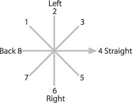
Now that we know which directions are possible, we want to take the current direction of movement into consideration. We want to keep the troll moving in the same general direction. We want to turn only when we have to, and even then a turn to the left or right is preferable to a complete change in direction. In this demo, we assign a number to each direction so that we can track the current direction. Figure 6-12 shows the numbers assigned to each direction.
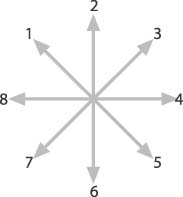
We will use the numbers shown in Figure 6-12 to record the direction of the move each time we update the troll’s position. This enables us to give added weight to the previous direction whenever it is time to update the troll’s position. Example 6-9 shows how this is accomplished.
if (entityList[i].direction==1)
    {
      terrainAnalysis[1]=terrainAnalysis[1]+2;
      terrainAnalysis[2]++;
      terrainAnalysis[5]--;
      terrainAnalysis[8]++;
    }
if (entityList[i].direction==2)
   {
      terrainAnalysis[1]++;
      terrainAnalysis[2]=terrainAnalysis[2]+2;
      terrainAnalysis[3]++;
      terrainAnalysis[6]--;
   }
if (entityList[i].direction==3)
   {
      terrainAnalysis[2]++;
      terrainAnalysis[3]=terrainAnalysis[3]+2;
      terrainAnalysis[4]++;
      terrainAnalysis[7]--;
   }
if (entityList[i].direction==4)
   {
      terrainAnalysis[3]++;
      terrainAnalysis[4]=terrainAnalysis[4]+2;
      terrainAnalysis[5]++;
      terrainAnalysis[7]--;
   }
if (entityList[i].direction==5)
   {
      terrainAnalysis[4]++;
      terrainAnalysis[5]=terrainAnalysis[5]+1;
      terrainAnalysis[6]++;
      terrainAnalysis[8]--;
   }
if (entityList[i].direction==6)
   {
      terrainAnalysis[2]--;
      terrainAnalysis[5]++;
      terrainAnalysis[6]=terrainAnalysis[6]+2;
      terrainAnalysis[7]++;
   }
if (entityList[i].direction==7)
   {
      terrainAnalysis[3]--;
      terrainAnalysis[6]++;
      terrainAnalysis[7]=terrainAnalysis[7]+2;
      terrainAnalysis[8]++;
   }
if (entityList[i].direction==8)
   {
      terrainAnalysis[1]++;
      terrainAnalysis[4]--;
      terrainAnalysis[7]++;
      terrainAnalysis[8]=terrainAnalysis[8]+2;
   }
decrease the weight of that element of the terrainAnalysis array by a value of 1. This example is illustrated in Figure 6-13.
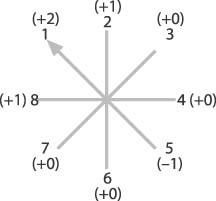
As Figure 6-13 shows, the current direction is 1, or up and left. All things being equal, we want the troll to continue in that direction, so the terrainAnalysis element is weighted with a +2. The two next best possibilities are directions 2 and 8 because those are the least severe turns. Those two are weighted with a +1. All the remaining elements are left as is, except for 5, which is the complete opposite direction. The next step is to choose the best direction. This is demonstrated in Example 6-10.
maxTerrain=0;
maxIndex=0;
for (j=1;j<=8;j++)
   if    (terrainAnalysis[j]>maxTerrain)
         {
            maxTerrain=terrainAnalysis[j];
            maxIndex=j;
         }
As Example 6-10 shows, we traverse the terrainAnalysis array in search of the most highly weighted of the possible directions. Upon exit from the for loop, the variable maxIndex will contain the array index to the most highly weighted direction. Example 6-11 shows how we use the value in maxIndex to update the troll’s position.
if (maxIndex==1)
   {
      entityList[i].direction=1;
      entityList[i].row--;
      entityList[i].col--;
   }
if (maxIndex==2)
   {
      entityList[i].direction=2;
      entityList[i].row--;
   }
if (maxIndex==3)
   {
      entityList[i].direction=3;
      entityList[i].row--;
      entityList[i].col++;
   }
if (maxIndex==4)
   {
      entityList[i].direction=4;
      entityList[i].col++;
   }
if (maxIndex==5)
   {
      entityList[i].direction=5;
      entityList[i].row++;
      entityList[i].col++;
   }
if (maxIndex==6)
   {
      entityList[i].direction=6;
      entityList[i].row++;
   }
if (maxIndex==7)
   {
      entityList[i].direction=7;
      entityList[i].row++;
      entityList[i].col--;
   }
if (maxIndex==8)
   {
      entityList[i].direction=8;
      entityList[i].col--;
   }
The value in maxIndex indicates the new direction of the troll. We include an if statement for each of the possible eight directions. Once the desired direction is found, we update the value in entityList[i].direction. This becomes the previous direction for the next time the troll’s position needs to be updated. We then update the entityList[i].row and entityList[i].col values as needed. Figure 6-14 shows the path followed as the troll moves along the road.
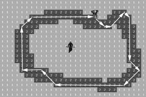
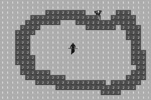
As Figure 6-14 shows, the troll continuously circles the road. In a real game, you could make the computer-controlled adversaries continuously patrol the roadways, until they encounter a player. At that point the computer-controlled character’s state could switch to an attack mode.
In this example, we used the adjacent tiles to make a weighted decision about direction to move in next. You can increase the robustness of this technique by examining more than just the adjacent tiles. You can weight the directions not just on the adjacent tiles, but also on the tiles adjacent to them. This could make the movement look even more natural and intelligent.
Wall Tracing
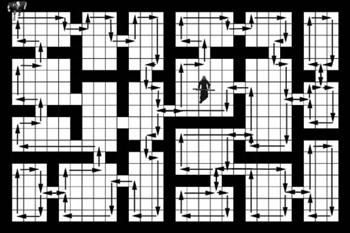
Another method of pathfinding that is very useful in game development is wall tracing. Like path-following, this method doesn’t calculate a path from a starting point to an ending point. Wall tracing is more of an exploration technique. It’s most useful in game environments made of many small rooms, although you can use it in maze-like game environments as well. You also can use the basic algorithm for tracing around obstacles, as we described in the previous section on obstacle tracing. Games rarely have every computer-controlled adversary simultaneously plotting a path to the player. Sometimes it’s desirable for the computer-controlled characters to explore the environment in search of the player, weapons, power-ups, treasure, or anything else a game character can interact with. Having the computer-controlled characters randomly move about the environment is one solution that game developers frequently implement. This offers a certain level of unpredictability, but it also can result in the computer-controlled characters getting stuck in small rooms for long periods of time. Figure 6-15 shows a dungeon-like level that’s made up of many small rooms.
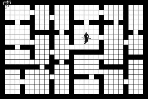
In the example shown in Figure 6-15, we could make the troll move in random directions. However, it would probably take it a while just to get out of the upper-left room. A better approach would be to make the troll systematically explore the entire environment. Fortunately, a relatively simple solution is available. Basically, we are going to use a lefthanded approach. If the troll always moves to its left, it will do a thorough job of exploring its environment. The trick is to remember that the troll needs to move to its left whenever possible, and not necessarily to the left from the point of view of the player. This is illustrated in Figure 6-16.
At the start of the demo, the troll is facing right relative to the player’s point of view. This is designated as direction 4, as shown in Figure 6-16. This means direction 2 is to the troll’s left, direction 6 is to the troll’s right, and direction 8 is to the troll’s rear. With the lefthanded movement approach, the troll always will try to move to its left first. If it can’t move to its left, it will try to move straight ahead. If that is blocked, it will try to move to its right next. If that also is blocked, it will reverse direction. When the demo first starts, the troll will try to move up relative to the player’s point of view. As you can see in Figure 6-15, a wall blocks its way, so the troll must try straight ahead next. This is direction 4 relative to the troll’s point of view. No obstruction appears straight ahead of the troll, so it makes the move. This lefthanded movement technique is shown in Example 6-12.
r=entityList[i].row;
c=entityList[i].col;
if (entityList[i].direction==4)
    {
       if (terrain[r-1][c]==1)
          {
             entityList[i].row--;
             entityList[i].direction=2;
          }
       else if (terrain[r][c+1]==1)
          {
             entityList[i].col++;
             entityList[i].direction=4;
          }
      else if (terrain[r+1][c]==1)
          {
             entityList[i].row++;
             entityList[i].direction=6;
          }
      else if (terrain[r][c-1]==1)
          {
             entityList[i].col--;
             entityList[i].direction=8;
          }
   }
else if (entityList[i].direction==6)
   {
      if (terrain[r][c+1]==1)
         {
            entityList[i].col++;
            entityList[i].direction=4;
         }
      else if (terrain[r+1][c]==1)
         {
            entityList[i].row++;
            entityList[i].direction=6;
         }
      else if (terrain[r][c-1]==1)
         {
            entityList[i].col--;
            entityList[i].direction=8;
         }
      else if (terrain[r-1][c]==1)
         {
            entityList[i].row--;
            entityList[i].direction=2;
         }
   }
else if (entityList[i].direction==8)
   {
      if (terrain[r+1][c]==1)
         {
            entityList[i].row++;
            entityList[i].direction=6;
         }
      else if (terrain[r][c-1]==1)
         {
            entityList[i].col--;
            entityList[i].direction=8;
         }
      else if (terrain[r-1][c]==1)
         {
            entityList[i].row--;
            entityList[i].direction=2;
         }
      else if (terrain[r][c+1]==1)
         {
            entityList[i].col++;
            entityList[i].direction=4;
         }
   }
else if (entityList[i].direction==2)
   {
      if (terrain[r][c-1]==1)
         {
            entityList[i].col--;
            entityList[i].direction=8;
         }
      else if (terrain[r-1][c]==1)
         {
            entityList[i].row--;
            entityList[i].direction=2;
         }
      else if (terrain[r][c+1]==1)
         {
            entityList[i].col++;
            entityList[i].direction=4;
         }
      else if (terrain[r+1][c]==1)
         {
            entityList[i].row++;
            entityList[i].direction=6;
         }
   }
Example 6-12 shows four separate if statement blocks. We need to use a different if block for each of the four possible directions in which the troll can face. This is required because the tile to the troll’s left is dependent on the direction it’s facing. This fact is illustrated in Figure 6-17.
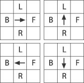
As Figure 6-17 shows, if the troll is facing the right relative to the player’s point of view, its left is the tile above it. If it’s facing up, the tile to its left is actually the tile on the left side. If it’s facing left, the tile below it is to its left. Finally, if it’s facing down, the tile to the right is the troll’s left.
As the first if block shows, if the troll is facing right, designated as direction 4, it first checks the tile to its left by examining terrain[r-1][c]. If this location contains a 1, there is no obstruction. At this point, the troll’s position is updated, and just as important, its direction is updated to 2. This means that it’s now facing up relative to the player’s point of view. The next time this block of code is executed, a different if block will be used because its direction has changed. The additional if statements ensure that the same procedure is followed for each possible direction.
If the first check of terrain[r-1][c] detected an obstruction, the tile in front of the troll would have been checked next. If that also contained an obstruction, the tile to the troll’s right would have been checked, followed by the tile to its rear. The end result is that the troll will thoroughly explore the game environment. This is illustrated in Figure 6-18.
As you can see, following the left-handed movement method, the troll enters every room in the game environment. Although this approach is conceptually easy and in most cases very effective, it is not guaranteed to work in all cases. Some geometries will prevent this method from allowing the troll to reach every single room.
Waypoint Navigation
Pathfinding can be a very time-consuming and CPU-intensive operation. One way to reduce this problem is to precalculate paths whenever possible. Waypoint navigation reduces this problem by carefully placing nodes in the game environment and then using precalculated paths or inexpensive pathfinding methods to move between each node. Figure 6-19 illustrates how to place nodes on a simple map consisting of seven rooms.
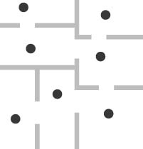
In Figure 6-19, you’ll notice that every point on the map is in the line of sight of at least one node. Also, every node is in the line of sight of at least one other node. With a game environment constructed in this way, a game-controlled character always will be able to reach any position on the map using a simple line-of-sight algorithm. The game AI simply needs to know how the nodes connect to one another. Figure 6-20 illustrates how to label and connect each node on the map.
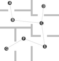
Using the node labels and links shown in Figure 6-20, we can now determine a path from any room to any other room. For example, moving from the room containing node A to the room containing node E entails moving through nodes ABCE. The path between nodes is calculated by a line-of-sight algorithm, or it can be a series of precalculated steps. Figure 6-21 shows how a computer-controlled character, indicated by the triangle, would calculate a path to the player-controlled character, indicated by the square.
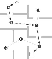
The computer-controlled character first calculates which node is nearest its current location and in its line of sight. In this case, that is node A. It then calculates which node is nearest the player’s current location and in the player’s line of sight. That is node E. The computer then plots a course from its current position to node A. Then it follows the node connections from node A to node E. In this case, that is A → B → C → E. Once it reaches the end node, it can plot a line-of-sight path from the final node to the player.
This seems simple enough, but how does the computer know which nodes to follow? In other words, how does the computer know that to get from node A to node E, it must first pass through nodes B and C? The answer lies in a simple table format for the data that enables us to quickly and easily determine the shortest path between any two nodes. Figure 6-22 shows our initial empty node connection table.
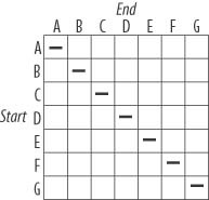
The purpose of the table is to establish the connections between the nodes. Filling in the table becomes a simple matter of determining the first node to visit when moving from any starting node to any ending node. The starting nodes are listed along the left side of the table, while the ending notes are shown across the top. We will determine the best path to follow by looking at the intersection on the table between the starting and ending nodes. You’ll notice that the diagonal on the table contains dashes. These table elements don’t need to be filled in because the starting and ending positions are equal. Take the upper-left table element, for example. Both the starting and ending nodes are A. You will never have to move from node A to node A, so that element is left blank. The next table element in the top row, however, shows a starting node of A and an ending node of B. We now look at Figure 6-21 to determine the first step to make when moving from node A to node B. In this case, the next move is to node B, so we fill in B on the second element of the top row. The next table element shows a starting node of A and an ending node of C. Again, Figure 6-21 shows us that the first step to take is to node B. When filling in the table we aren’t concerned with determining the entire path between every two nodes. We only need to determine the first node to visit when moving from any node to any other node. Figure 6-23 shows the first table row completed.
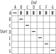
Figure 6-23 shows us that when moving from node A to any other node, we must first visit node B. Examining Figure 6-21 confirms this fact. The only node connected to node A is node B, so we must always pass through node B when moving from node A to any other node. Simply knowing that we must visit node B when moving from node A to node E doesn’t get us to the destination. We must finish filling in the table. Moving to the second row in the table, we see that moving from node B to node A requires a move to node A. Moving from node B to node C requires a move to C. We continue doing this until each element in the table is complete. Figure 6-24 shows the completed node connection table.
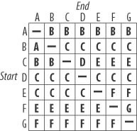
By using the completed table shown in Figure 6-24, we can determine the path to follow to get from any node to any other node. Figure 6-25 shows an example of a desired path. In this figure, a hypothetical computer-controlled character, indicated by the triangle, wants to build a path to the player, indicated by the square.
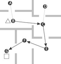
To build a path we simply need to refer to the completed node connection table shown in Figure 6-24. As shown in Figure 6-25, we want to build a path from node B to node G. We start by finding the intersection on the table between node B and node G. The table shows node C at the intersection. So, the first link to traverse when moving from node B to node G is B → C. Once we arrive at node C, we refer to the table again to find the intersection between node C and the desired destination, node G. In the case, we find node E at the intersection. We then proceed to move from C → E. We repeat this process until the destination is reached. Figure 6-26 shows the individual path segments that are followed when building a path from node B to node G.
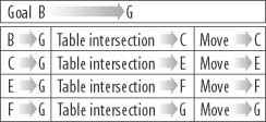
As Figure 6-26 shows, the computer-controlled character needs to follow four path segments to reach its destination.
Each method we discussed here has its advantages and disadvantages, and it’s clear that no single method is best suited for all possible pathfinding problems. Another method we mentioned at the beginning of this chapter, the A∗ algorithm, is applicable to a wide range of pathfinding problems. The A∗ algorithm is an extremely popular pathfinding algorithm used in games, and we devote the entire next chapter to the method.