
Chapter 3. Pattern Movement
This chapter covers the subject of pattern movement. Pattern movement is a simple way to give the illusion of intelligent behavior. Basically, the computer-controlled characters move according to some predefined pattern that makes it appear as though they are performing complex, thought-out maneuvers. If you’re old enough to remember the classic arcade game Galaga, you’ll immediately know what pattern movement is all about. Recall the alien ships swooping down from the top and in from the sides of the screen, performing loops and turns, all the while shooting at your ship. The aliens, depending on their type and the level you were on, were capable of different maneuvers. These maneuvers were achieved using pattern movement algorithms.
Although Galaga is a classic example of using pattern movement, even modern video games use some form of pattern movement. For example, in a role-playing game or first-person shooter game, enemy monsters might patrol areas within the game world according to some predefined pattern. In a flight combat simulation, the enemy aircraft might perform evasive maneuvers according to some predefined patterns. Secondary creatures and nonplayer characters in different genres can be programmed to move in some predefined pattern to give the impression that they are wandering, feeding, or performing some task.
The standard method for implementing pattern movement takes the desired pattern and encodes the control data into an array or set of arrays. The control data consists of specific movement instructions, such as move forward and turn, that force the computer-controlled object or character to move according to the desired pattern. Using these algorithms, you can create a circle, square, zigzag, curve—any type of pattern that you can encode into a concise set of movement instructions.
In this chapter, we’ll go over the standard pattern movement algorithm in generic terms before moving on to two examples that implement variations of the standard algorithm. The first example is tile-based, while the second shows how to implement pattern movement in physically simulated environments in which you must consider certain caveats specific to such environments.
Standard Algorithm
The standard pattern movement algorithm uses lists or arrays of encoded instructions, or control instructions, that tell the computer-controlled character how to move each step through the game loop. The array is indexed each time through the loop so that a new set of movement instructions gets processed each time through.
Example 3-1 shows a typical set of control instructions.
 ControlData {
     double turnRight;
     double turnLeft;
     double stepForward;
     double stepBackward;
     };
In this example, turnRight and turnLeft would contain the number of degrees by which to turn right or left. If this were a tile-based game in which the number of directions in which a character could head is limited, turnRight and turnLeft could mean turn right or left by one increment. stepForward and stepBackward would contain the number of distance units, or tiles, by which to step forward or backward.
This control structure also could include other instructions, such as fire weapon, drop bomb, release chaff, do nothing, speed up, and slow down, among many other actions appropriate to your game.
Typically you set up a global array or set of arrays of the control structure type to store the pattern data. The data used to initialize these pattern arrays can be loaded in from a data file or can be hardcoded within the game; it really depends on your coding style and on your game’s requirements.
Initialization of a pattern array, one that was hardcoded, might look something such as that shown in Example 3-2.
Pattern[0].turnRight = 0;
Pattern[0].turnLeft = 0;
Pattern[0].stepForward = 2;
Pattern[0].stepBackward = 0;
Pattern[1].turnRight = 0;
Pattern[1].turnLeft = 0;
Pattern[1].stepForward = 2;
Pattern[1].stepBackward = 0;
Pattern[2].turnRight = 10;
Pattern[2].turnLeft = 0;
Pattern[2].stepForward = 0;
Pattern[2].stepBackward = 0;
Pattern[3].turnRight = 10;
Pattern[3].turnLeft = 0;
Pattern[3].stepForward = 0;
Pattern[3].stepBackward = 0;
Pattern[4].turnRight = 0;
Pattern[4].turnLeft = 0;
Pattern[4].stepForward = 2;
Pattern[4].stepBackward = 0;
Pattern[5].turnRight = 0;
Pattern[5].turnLeft = 0;
Pattern[5].stepForward = 2;
Pattern[5].stepBackward = 0;
Pattern[6].turnRight = 0;
Pattern[6].turnLeft = 10;
Pattern[6].stepForward = 0;
Pattern[6].stepBackward = 0;
                 .
                 .
                 .
In this example, the pattern instructs the computer-controlled character to move forward 2 distance units, move forward again 2 distance units, turn right 10 degrees, turn right again 10 degrees, move forward 2 distance units, move forward again 2 distance units, and turn left 10 degrees. This specific pattern causes the computer-controlled character to move in a zigzag pattern.
To process this pattern, you need to maintain and increment an index to the pattern array each time through the game loop. Further, each time through the loop, the control instructions corresponding to the current index in the pattern array must be read and executed. Example 3-3 shows how such steps might look in code.
void     GameLoop(void)
{
     .
     .
     .
     Object.orientation + = Pattern[CurrentIndex].turnRight;
     Object.orientation -- = Pattern[CurrentIndex].turnLeft;
     Object.x + = Pattern[CurrentIndex].stepForward;
     Object.x -- = Pattern[CurrentIndex].stepBackward;
     CurrentIndex++;
     .
     .
     .
}
As you can see, the basic algorithm is fairly simple. Of course, implementation details will vary depending on the structure of your game.
It’s also common practice to encode several different patterns in different arrays and have the computer select a pattern to execute at random or via some other decision logic within the game. Such techniques enhance the illusion of intelligence and lend more variety to the computer-controlled character’s behavior.
Pattern Movement in Tiled Environments
The approach we’re going to use for tile-based pattern movement is similar to the method we used for tile-based line-of-sight chasing in Chapter 2. In the line-of-sight example, we used Bresenham’s line algorithm to precalculate a path between a starting point and an ending point. In this chapter, we’re going to use Bresenham’s line algorithm to calculate various patterns of movement. As we did in Chapter 2, we’ll store the row and column positions in a set of arrays. These arrays can then be traversed to move the computer-controlled character, a troll in this example, in various patterns.
In this chapter, paths will be more complex than just a starting point and an ending point. Paths will be made up of line segments. Each new segment will begin where the previous one ended. You need to make sure the last segment ends where the first one begins to make the troll moves in a repeating pattern. This method is particularly useful when the troll is in a guarding or patrolling mode. For example, you could have the troll continuously walk around the perimeter of a campsite and then break free of the pattern only if an enemy enters the vicinity. In this case, you could use a simple rectangular pattern.
You can accomplish this rectangular pattern movement by simply calculating four line segments. In Chapter 2, the line-of-sight function cleared the contents of the row and column path arrays each time it was executed. In this case, however, each line is only a segment of the overall pattern. Therefore, we don’t want to initialize the path arrays each time a segment is calculated, but rather, append each new line path to the previous one. In this example, we’re going to initialize the row and column arrays before the pattern is calculated. Example 3-4 shows the function that we used to initialize the row and column path arrays.
void    InitializePathArrays(void)
{
     int i;
     for (i=0;i<kMaxPathLength;i++)
           {
                  pathRow[i] = --1;
                  pathCol[i] = --1;
          }
}
As Example 3-4 shows, we initialize each element of both arrays to a value of −1. We use −1 because it’s not a valid coordinate in the tile-based environment. Typically, in most tile-based environments, the upper leftmost coordinate is (0,0). From that point, the row and column coordinates increase to the size of the tile map. Setting unused elements in the path arrays to −1 is a simple way to indicate which elements in the path arrays are not used. This is useful when appending one line segment to the next in the path arrays. Example 3-5 shows the modified Bresenham line-of-sight algorithm that is used to calculate line segments.
void ai_Entity::BuildPathSegment(void)
{
     int i;
     int nextCol=col;
     int nextRow=row;
     int deltaRow=endRow-row;
     int deltaCol=endCol-col;
     int stepCol;
     int stepRow;
     int currentStep;
     int fraction;
     int i;
     for (i=0;i<kMaxPathLength;i++)
           if ((pathRow[i]==-1) && (pathCol[i]==1))
                {
                       currentStep=i;
                       break;
               }
     if (deltaRow < 0) stepRow=-1; else stepRow=1;
     if (deltaCol < 0) stepCol=-1; else stepCol=1;
     deltaRow=abs(deltaRow*2);
     deltaCol=abs(deltaCol*2);
     pathRow[currentStep]=nextRow;
     pathCol[currentStep]=nextCol;
     currentStep++;
     if (currentStep>=kMaxPathLength)
          return;
     if (deltaCol > deltaRow)
          {
               fraction = deltaRow * 2 - deltaCol;
               while (nextCol != endCol)
                    {
                         if (fraction >= 0)
                              {
                                   nextRow += stepRow;
                                   fraction = fraction - deltaCol;
                              }
                         nextCol = nextCol + stepCol;
                         fraction = fraction + deltaRow;
                         pathRow[currentStep]=nextRow;
                         pathCol[currentStep]=nextCol;
                         currentStep++;
                         if (currentStep>=kMaxPathLength)
                              return;
                    }
          }
     else
          {
               fraction = deltaCol * 2 - deltaRow;
               while (nextRow != endRow)
                    {
                         if (fraction >= 0)
                              {
                                   nextCol = nextCol + stepCol;
                                   fraction = fraction - deltaRow;
                              }
                         nextRow = nextRow + stepRow;
                         fraction = fraction + deltaCol;
                         pathRow[currentStep]=nextRow;
                         pathCol[currentStep]=nextCol;
                         currentStep++;
                         if (currentStep>=kMaxPathLength)
                              return;
                    }
          }
}
For the most part, this algorithm is very similar to the line-of-sight movement algorithm shown in Example 2-7 from Chapter 2. The major difference is that we replaced the section of code that initializes the path arrays with a new section of code. In this case, we want each new line segment to be appended to the previous one, so we don’t want to initialize the path arrays each time this function is called. The new section of code determines where to begin appending the line segment. This is where we rely on the fact that we used a value of −1 to initialize the path arrays. All you need to do is simply traverse the arrays and check for the first occurrence of the value −1. This is where the new line segment begins. Using the function in Example 3-6, we’re now ready to calculate the first pattern. Here, we’re going to use a simple rectangular patrolling pattern. Figure 3-1 shows the desired pattern.
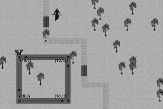
As you can see in Figure 3-1, we highlighted the vertex coordinates of the rectangular pattern, along with the desired direction of movement. Using this information, we can establish the troll’s pattern using the BuildPathSegment function from Example 3-5. Example 3-6 shows how the rectangular pattern is initialized.
     entityList[1].InitializePathArrays();
     entityList[1].BuildPathSegment(10, 3, 18, 3);
     entityList[1].BuildPathSegment(18, 3, 18, 12);
     entityList[1].BuildPathSegment(18, 12, 10, 12);
     entityList[1].BuildPathSegment(10, 12, 10, 3);
     entityList[1].NormalizePattern();
     entityList[1].patternRowOffset = 5;
     entityList[1].patternColOffset = 2;
As you can see in Example 3-6, you first initialize the path arrays by calling the function InitializePathArrays. Then you use the coordinates shown in Figure 3-1 to calculate the four line segments that make up the rectangular pattern. After each line segment is calculated and stored in the path arrays, we make a call to NormalizePattern to adjust the resulting pattern so that it is represented in terms of relative coordinates instead of absolute coordinates. We do this so that the pattern is not tied to any specific starting position in the game world. Once the pattern is built and normalized, we can execute it from anywhere. Example 3-7 shows the NormalizePattern function.
void ai_Entity::NormalizePattern(void)
{
     int i;
     int rowOrigin=pathRow[0];
     int colOrigin=pathCol[0];
     for (i=0;i<kMaxPathLength;i++)
     	    if ((pathRow[i]==-1) && (pathCol[i]==-1))
     		           {
     		                pathSize=i-1;
     		                break;
		                }

     for (i=0;i<=pathSize;i++)
            {
                  pathRow[i]=pathRow[i]-rowOrigin;
                  pathCol[i]=pathCol[i]-colOrigin;
            }
}
As you can see, all we do to normalize a pattern is subtract the starting position from all the positions stored in the pattern arrays. This yields a pattern in terms of relative coordinates so that we can execute it from anywhere in the game world.
Now that the pattern has been constructed we can traverse the arrays to make the troll walk in the rectangular pattern. You’ll notice that the last two coordinates in the final segment are equal to the first two coordinates of the first line segment. This ensures that the troll walks in a repeating pattern.
You can construct any number of patterns using the BuildPathSegment function. You simply need to determine the vertex coordinates of the desired pattern and then calculate each line segment. Of course, you can use as few as two line segments or as many line segments as the program resources allow to create a movement pattern. Example 3-8 shows how you can use just two line segments to create a simple back-and-forth patrolling pattern.
     entityList[1].InitializePathArrays();
     entityList[1].BuildPathSegment(10, 3, 18, 3);
     entityList[1].BuildPathSegment(18, 3, 10, 3);
     entityList[1].NormalizePattern();
     entityList[1].patternRowOffset = 5;
     entityList[1].patternColOffset = 2;
Using the line segments shown in Example 3-8, the troll simply walks back and forth between coordinates (10,3) and (18,3). This could be useful for such tasks as patrolling near the front gate of a castle or protecting an area near a bridge. The troll could continuously repeat the pattern until an enemy comes within sight. The troll could then switch to a chasing or attacking state.
Of course, there is no real limit to how many line segments you can use to generate a movement pattern. You can use large and complex patterns for such tasks as patrolling the perimeter of a castle or continuously marching along a shoreline to guard against invaders. Example 3-9 shows a more complex pattern. This example creates a pattern made up of eight line segments.
     entityList[1].BuildPathSegment(4, 2, 4, 11);
     entityList[1].BuildPathSegment(4, 11, 2, 24);
     entityList[1].BuildPathSegment(2, 24, 13, 27);
     entityList[1].BuildPathSegment(13, 27, 16, 24);
     entityList[1].BuildPathSegment(16, 24, 13, 17);
     entityList[1].BuildPathSegment(13, 17, 13, 13);
     entityList[1].BuildPathSegment(13, 13, 17, 5);
     entityList[1].BuildPathSegment(17, 5, 4, 2);
     entityList[1].NormalizePattern();
     entityList[1].patternRowOffset = 5;
     entityList[1].patternColOffset = 2;
Example 3-9 sets up a complex pattern that takes terrain elements into consideration. The troll starts on the west bank of the river, crosses the north bridge, patrols to the south, crosses the south bridge, and then returns to its starting point to the north. The troll then repeats the pattern. Figure 3-2 shows the pattern, along with the vertex points used to construct it.
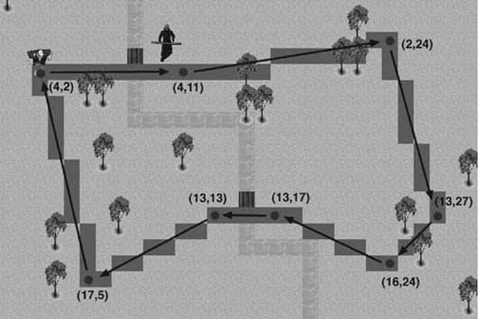
As Figure 3-2 shows, this method of pattern movement allows for very long and complex patterns. This can be particularly useful when setting up long patrols around various terrain elements.
Although the pattern method used in Figure 3-2 can produce long and complex patterns, these patterns can appear rather repetitive and predictable. The next method we’ll look at adds a random factor, while still maintaining a movement pattern. In a tile-based environment, the game world typically is represented by a two-dimensional array. The elements in the array indicate which object is located at each row and column coordinate. For this next pattern movement method, we’ll use a second two-dimensional array. This pattern matrix guides the troll along a predefined track. Each element of the pattern array contains either a 0 or a 1. The troll is allowed to move to a row and column coordinate only if the corresponding element in the pattern array contains a 1.
The first thing you must do to implement this type of pattern movement is to set up a pattern matrix. As Example 3-10 shows, you start by initializing the pattern matrix to all 0s.
     for (i=0;i<kMaxRows;i++)
          for (j=0;j<kMaxCols;j++)
               pattern[i][j]=0;
After the entire pattern matrix is set to 0, you can begin setting the coordinates of the desired movement pattern to 1s. We’re going to create a pattern by using another variation of the Bresenham line-of-sight algorithm that we used in Chapter 2. In this case, however, we’re not going to save the row and column coordinates in path arrays. We’re going to set the pattern matrix to 1 at each row and column coordinate along the line. We can then make multiple calls to the pattern line function to create complex patterns. Example 3-11 shows a way to set up one such pattern.
     BuildPatternSegment(3, 2, 16, 2);
     BuildPatternSegment(16, 2, 16, 11);
     BuildPatternSegment(16, 11, 9, 11);
     BuildPatternSegment(9, 11, 9, 2);
     BuildPatternSegment(9, 6, 3, 6);
     BuildPatternSegment(3, 6, 3, 2);
Each call to the BuildPatternSegment function uses the Bresenham line algorithm to draw a new line segment to the pattern matrix. The first two function parameters are the row and column of the starting point, while the last two are the row and column of the ending point. Each point in the line becomes a 1 in the pattern matrix. This pattern is illustrated in Figure 3-3.
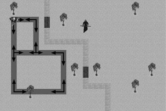
Figure 3-3 highlights each point where the pattern matrix contains a 1. These are the locations where the troll is allowed to move. You’ll notice, however, that at certain points along the track there is more than one valid direction for the troll. We’re going to rely on this fact to make the troll move in a less repetitive and predictable fashion.
Whenever it’s time to update the troll’s position, we’ll check each of the eight surrounding elements in the pattern array to determine which are valid moves. This is demonstrated in Example 3-12.
void ai_Entity::FollowPattern(void)
{
     int i,j;
     int possibleRowPath[8]={0,0,0,0,0,0,0,0};
     int possibleColPath[8]={0,0,0,0,0,0,0,0};
     int rowOffset[8]={-1,-1,-1, 0, 0, 1, 1, 1};
     int colOffset[8]={-1, 0, 1,-1, 1,-1, 0, 1};
     j=0;
     for (i=0;i<8;i++)
          if (pattern[row+rowOffset[i]][col+colOffset[i]]==1)
               if (!(((row+rowOffset[i])==previousRow) &&
                    ((col+colOffset[i])==previousCol)))
                    {
                         possibleRowPath[j]=row+rowOffset[i];
                         possibleColPath[j]=col+colOffset[i];
                         j++;
                    }
     i=Rnd(0,j-1);
     previousRow=row;
     previousCol=col;
     row=possibleRowPath[i];
     col=possibleColPath[i];
You start by checking the pattern matrix at each of the eight points around the troll’s current position. Whenever you find a value of 1, you save that coordinate to the possibleRowPath and possibleColPath arrays. After each point is checked, you randomly select a new coordinate from the array of valid points found. The end result is that the troll won’t always turn in the same direction when it reaches an intersection in the pattern matrix.
Note that the purpose of the rowOffset and colOffset variables shown in Example 3-12 is to avoid having to write eight conditional statements. Using a loop and adding these values to the row and column position traverses the eight adjacent tiles. For example, the first two elements, when added to the current row and column, are the tiles to the upper left of the current position.
You have to consider one other point when moving the troll. The troll’s previous location always will be in the array of valid moves. Selecting that point can lead to an abrupt back-and-forth movement when updating the troll’s position. Therefore, you should always track the troll’s previous location using the previousRow and previousCol variables. Then you can exclude that position when building the array of valid moves.
Pattern Movement in Physically Simulated Environments
So far in this chapter we discussed how to implement patterned movement in environments where you can instruct your game characters to take discrete steps or turns; but what about physically simulated environments? Surely you can take advantage of the utility of pattern movement in physically simulated environments as well. The trouble is that the benefit of using physically simulated environments—namely, letting the physics take control of movement—isn’t conducive to forcing a physically simulated object to follow a specific pattern of movement. Forcing a physically simulated aircraft, for example, to a specific position or orientation each time through the game loop defeats the purpose of the underlying physical simulation. In physically simulated environments, you don’t specify an object’s position explicitly during the simulation. So, to implement pattern movement in this case, you need to revise the algorithms we discussed earlier. Specifically, rather than use patterns that set an object’s position and orientation each time through the game loop, you need to apply appropriate control forces to the object to coax it, or essentially drive it, to where you want it to go.
You saw in the second example in Chapter 2 how we used steering forces to make the predator chase his prey. You can use these same steering forces to drive your physically simulated objects so that they follow some pattern. This is, in fact, an approximation to simulating an intelligent creature at the helm of such a physically simulated vehicle. By applying control forces, you essentially are mimicking the behavior of the driver piloting his vehicle in some pattern. The pattern can be anything—evasive maneuvers, patrol paths, stunts—so long as you can apply the appropriate control forces, such as thrust and steering forces.
Keep in mind, however, that you don’t have absolute control in this case. The physics engine and the model that governs the capabilities—such as speed and turning radius, among others—of the object being simulated still control the object’s overall behavior. Your input in the form of steering forces and thrust modulation, for example, is processed by the physics engine, and the resulting behavior is a function of all inputs to the physics engine, not just yours. By letting the physics engine maintain control, we can give the computer-controlled object some sense of intelligence without forcing the object to do something the physics model does not allow. If you violate the physics model, you run the risk of ruining the immersive experience realistic physics create. Remember, our goal is to enhance that immersiveness with the addition of intelligence.
To demonstrate how to implement path movement in the context of physically simulated environments, we’re going to use as a basis the scenario we described in Chapter 2 for chasing and intercepting in continuous environments. Recall that this scenario included two vehicles that we simulated using a simple two-dimensional rigid-body simulation. The computer controlled one vehicle, while the player controlled the other. In this chapter, we’re going to modify that example, demonstration program AIDemo2-2, such that the computer-controlled vehicle moves according to predefined patterns. The resulting demonstration program is entitled AIDemo3-2, and you can download it from this book’s Web site.
The approach we’ll take in this example is very similar to the algorithms we discussed earlier. We’ll use an array to store the pattern information and then step through this array, giving the appropriate pattern instructions to the computer-controlled vehicle. There are some key differences between the algorithms we discussed earlier and the one required for physics-based simulations. In the earlier algorithms, the pattern arrays stored discrete movement information—take a step left, move a step forward, turn right, turn left, and so on. Further, each time through the game loop the pattern array index was advanced so that the next move’s instructions could be fetched. In physics-based simulations, you must take a different approach, which we discuss in detail in the next section.
Control Structures
As we mentioned earlier, in physics-based simulations you can’t force the computer-controlled vehicle to make a discrete step forward or backward. Nor can you tell it explicitly to turn left or right. Instead, you have to feed the physics engine control force information that, in effect, pilots the computer-controlled vehicle in the pattern you desire. Further, when a control force—say, a steering force—is applied in physics-based simulations, it does not instantaneously change the motion of the object being simulated. These control forces have to act over time to effect the desired motion. This means you don’t have a direct correspondence between the pattern array indices and game loop cycles; you wouldn’t want that anyway. If you have a pattern array that contains a specific set of instructions to be executed each time you step through the simulation, the pattern arrays would be huge because the time steps typically taken in a physics-based simulation are very small.
To get around this, the control information contained in the pattern arrays we use here also contains information so that the computer knows how long, so to speak, each set of instructions should be applied. The algorithm works like this: the computer selects the first set of instructions from the pattern array and applies them to the vehicle being controlled. The physics engine processes those instructions each time step through the simulation until the conditions specified in the given set of instructions are met. At that point the next set of instructions from the pattern array are selected and applied. This process repeats all the way through the pattern array, or until the pattern is aborted for some other reason.
The code in Example 3-13 shows the pattern control data structure we set up for this example.
struct    ControlData {
     bool     PThrusterActive;
     bool     SThrusterActive;
     double   dHeadingLimit;
     double   dPositionLimit;
     bool     LimitHeadingChange;
     bool     LimitPositionChange;
};
Be aware that this control data will vary depending on what you are simulating in your game and how its underlying physics model works. In this case, the vehicle we’re controlling is steered only by bow thruster forces. Thus, these are the only two control forces at our disposal with which we can implement some sort of pattern movement.
Therefore, the data structure shown in Example 3-13 contains two boolean members, PThrusterActive and SThrusterActive, which indicate whether each thruster should be activated. The next two members, dHeadingLimit and dPositionLimit, are used to determine how long each set of controls should be applied. For example, dHeadingLimit specifies a desired change in the vehicle’s heading. If you want a particular instruction to turn the vehicle 45 degrees, you set this dHeadingLimit to 45. Note that this is a relative change in heading and not an absolute orientation. If the flag LimitHeadingChange is set to true, dHeadingLimit is checked each time through the simulation loop while the given pattern instruction is being applied. If the vehicle’s heading has changed sufficiently relative to its last heading before this instruction was applied, the next instruction should be fetched.
Similar logic applies to dPositionLimit. This member stores the desired change in position—that is, distance traveled relative to the position of the vehicle before the given set of instructions was applied. If LimitPositionChange is set to true, each time through the simulation loop the relative position change of the vehicle is checked against dPositionChange to determine if the next set of instructions should be fetched from the pattern array.
Before proceeding further, let us stress that the pattern movement algorithm we’re showing you here works with relative changes in heading and position. The pattern instructions will be something such as move forward 100 ft, then turn 45 degrees to the left, then move forward another 100 ft, then turn 45 degrees to the right, and so on. The instructions will be absolute: move forward until you reach position (x, y)0, then turn until you are facing southeast, then move until you reach position (x, y)1, then turn until you are facing southwest, and so on.
Using relative changes in position and heading enables you to execute the stored pattern regardless of the location or initial orientation of the object being controlled. If you were to use absolute coordinates and compass directions, the patterns you use would be restricted near those coordinates. For example, you could patrol a specific area on a map using some form of pattern, but you would not be able to patrol any area on a map with the specific pattern. The latter approach, using absolute coordinates, is consistent with the algorithm we showed you in the previous tile-based example. Further, such an approach is in line with waypoint navigation, which has its own merits, as we discuss in later chapters.
Because we’re using relative changes in position and heading here, you also need some means of tracking these changes from one set of pattern instructions to the next. To this end, we defined another structure that stores the changes in state of the vehicle from one set of pattern instructions to the next. Example 3-14 shows the structure.
struct    StateChangeData {
     Vector     InitialHeading;
     Vector     InitialPosition;
     double     dHeading;
     double     dPosition;
     int        CurrentControlID;
};
The first two members, InitialHeading and InitialPosition, are vectors that store the heading and position of the vehicle being controlled at the moment a set of pattern instructions is selected from the pattern array. Every time the pattern array index is advanced and a new set of instructions is fetched, these two members must be updated. The next two members, dHeading and dPosition, store the changes in position and heading as the current set of pattern instructions is being applied during the simulation. Finally, CurrentControlID stores the current index in the pattern array, which indicates the current set of pattern control instructions being executed.
Pattern Definition
Now, to define some patterns, you have to fill in an array of ControlData structures with appropriate steering control instructions corresponding to the desired movement pattern. For this example, we set up three patterns. The first is a square pattern, while the second is a zigzag pattern. In an actual game, you could use the square pattern to have the vehicle patrol an area bounded by the square. You could use the zigzag pattern to have the vehicle make evasive maneuvers, such as when Navy ships zigzag through the ocean to make it more difficult for enemy submarines to attack them with torpedoes. You can define control inputs for virtually any pattern you want to simulate; you can define circles, triangles, or any arbitrary path using this method. In fact, the third pattern we included in this example is an arbitrarily shaped pattern.
For the square and zigzag patterns, we set up two global arrays called PatrolPattern and ZigZagPattern, as shown in Example 3-15.
#define_PATROL_ARRAY_SIZE           8
#define _ZIGZAG_ARRAY_SIZE          4
ControlData          PatrolPattern[_PATROL_ARRAY_SIZE];
ControlData          ZigZagPattern[_ZIGZAG_ARRAY_SIZE];
StateChangeData      PatternTracking;
As you can see, we also defined a global variable called PatternTracking that tracks changes in position and heading as these patterns get executed.
Examples 3-16 and 3-17 show how each of these two patterns is initialized with the appropriate control data. We hardcoded the pattern initialization in this demo; however, in an actual game you might prefer to load in the pattern data from a data file. Further, you can optimize the data structure using a more concise encoding, as opposed to the structure we used here for the sake of clarity.
     PatrolPattern[0].LimitPositionChange = true;
     PatrolPattern[0].LimitHeadingChange = false;
     PatrolPattern[0].dHeadingLimit = 0;
     PatrolPattern[0].dPositionLimit = 200;
     PatrolPattern[0].PThrusterActive = false;
     PatrolPattern[0].SThrusterActive = false;
     PatrolPattern[1].LimitPositionChange = false;
     PatrolPattern[1].LimitHeadingChange = true;
     PatrolPattern[1].dHeadingLimit = 90;
     PatrolPattern[1].dPositionLimit = 0;
     PatrolPattern[1].PThrusterActive = true;
     PatrolPattern[1].SThrusterActive = false;
     PatrolPattern[2].LimitPositionChange = true;
     PatrolPattern[2].LimitHeadingChange = false;
     PatrolPattern[2].dHeadingLimit = 0;
     PatrolPattern[2].dPositionLimit = 200;
     PatrolPattern[2].PThrusterActive = false;
     PatrolPattern[2].SThrusterActive = false;
     PatrolPattern[3].LimitPositionChange = false;
     PatrolPattern[3].LimitHeadingChange = true;
     PatrolPattern[3].dHeadingLimit = 90;
     PatrolPattern[3].dPositionLimit = 0;
     PatrolPattern[3].PThrusterActive = true;
     PatrolPattern[3].SThrusterActive = false;
     PatrolPattern[4].LimitPositionChange = true;
     PatrolPattern[4].LimitHeadingChange = false;
     PatrolPattern[4].dHeadingLimit = 0;
     PatrolPattern[4].dPositionLimit = 200;
     PatrolPattern[4].PThrusterActive = false;
     PatrolPattern[4].SThrusterActive = false;
     PatrolPattern[5].LimitPositionChange = false;
     PatrolPattern[5].LimitHeadingChange = true;
     PatrolPattern[5].dHeadingLimit = 90;
     PatrolPattern[5].dPositionLimit = 0;
     PatrolPattern[5].PThrusterActive = true;
     PatrolPattern[5].SThrusterActive = false;
     PatrolPattern[6].LimitPositionChange = true;
     PatrolPattern[6].LimitHeadingChange = false;
     PatrolPattern[6].dHeadingLimit = 0;
     PatrolPattern[6].dPositionLimit = 200;
     PatrolPattern[6].PThrusterActive = false;
     PatrolPattern[6].SThrusterActive = false;
     PatrolPattern[7].LimitPositionChange = false;
     PatrolPattern[7].LimitHeadingChange = true;
     PatrolPattern[7].dHeadingLimit = 90;
     PatrolPattern[7].dPositionLimit = 0;
     PatrolPattern[7].PThrusterActive = true;
PatrolPattern[7].SThrusterActive = false; ZigZagPattern[0].LimitPositionChange = true;
ZigZagPattern[0].LimitHeadingChange = false;
ZigZagPattern[0].dHeadingLimit = 0;
ZigZagPattern[0].dPositionLimit = 100;
ZigZagPattern[0].PThrusterActive = false;
ZigZagPattern[0].SThrusterActive = false;
ZigZagPattern[1].LimitPositionChange = false;
ZigZagPattern[1].LimitHeadingChange = true;
ZigZagPattern[1].dHeadingLimit = 60;
ZigZagPattern[1].dPositionLimit = 0;
ZigZagPattern[1].PThrusterActive = true;
ZigZagPattern[1].SThrusterActive = false;
ZigZagPattern[2].LimitPositionChange = true;
ZigZagPattern[2].LimitHeadingChange = false;
ZigZagPattern[2].dHeadingLimit = 0;
ZigZagPattern[2].dPositionLimit = 100;
ZigZagPattern[2].PThrusterActive = false;
ZigZagPattern[2].SThrusterActive = false;
ZigZagPattern[3].LimitPositionChange = false;
ZigZagPattern[3].LimitHeadingChange = true;
ZigZagPattern[3].dHeadingLimit = 60;
ZigZagPattern[3].dPositionLimit = 0;
ZigZagPattern[3].PThrusterActive = false;
ZigZagPattern[3].SThrusterActive = true;The square pattern control inputs are fairly simple. The first set of instructions corresponding to array element [0] tells the vehicle to move forward by 200 distance units. In this case no steering forces are applied. Note here that the forward thrust acting on the vehicle already is activated and held constant. You could include thrust in the control structure for more complex patterns that include steering and speed changes.
The next set of pattern instructions, array element [1], tells the vehicle to turn right by activating the port bow thruster until the vehicle’s heading has changed 90 degrees. The instructions in element [2] are identical to those in element [0] and they tell the vehicle to continue straight for 200 distance units. The remaining elements are simply a repeat of the first three—element [3] makes another 90-degree right turn, element [4] heads straight for 200 distance units, and so on. The end result is eight sets of instructions in the array that pilot the vehicle in a square pattern.
In practice you could get away with only two sets of instructions, the first two shown in Example 3-16, and still achieve a square pattern. The only difference is that you’d have to repeat those two sets of instructions four times to form a square.
The zigzag controls are similar to the square controls in that the vehicle first moves forward a bit, then turns, then moves forward some more, and then turns again. However, this time the turns alternate from right to left, and the angle through which the vehicle turns is limited to 60 degrees rather than 90. The end result is that the vehicle moves in a zigzag fashion.
Executing the Patterns
In this example, we initialize the patterns in an Initialize function that gets called when the program first starts. Within that function, we also go ahead and initialize the PatternTracking structure by making a call to a function called InitializePatternTracking, which is shown in Example 3-18.
void InitializePatternTracking(void)
{
     PatternTracking.CurrentControlID = 0;
     PatternTracking.dPosition = 0;
     PatternTracking.dHeading = 0;
     PatternTracking.InitialPosition = Craft2.vPosition;
     PatternTracking.InitialHeading = Craft2.vVelocity;
     PatternTracking.InitialHeading.Normalize();
}
Whenever InitializePatternTracking is called, it copies the current position and velocity vectors for Craft2, the computer-controlled vehicle, and stores them in the state change data structure. The CurrentControlID, which is the index to the current element in the given pattern array, is set to 0, indicating the first element. Further, changes in position and heading are initialized to 0.
Of course, nothing happens if you don’t have a function that actually processes these instructions. So, to that end, we defined a function called DoPattern, which takes a pointer to a pattern array and the number of elements in the array as parameters. This function must be called every time through the simulation loop to apply the pattern controls and step through the pattern array. In this example, we make the call to DoPattern within the UpdateSimulation function as illustrated in Example 3-19.
void UpdateSimulation(void)
{
     .
     .
     .
     if(Patrol)
     {
          if(!DoPattern(PatrolPattern, _PATROL_ARRAY_SIZE))
               InitializePatternTracking();
     }
     if(ZigZag)
     {
          if(!DoPattern(ZigZagPattern, _ZIGZAG_ARRAY_SIZE))
               InitializePatternTracking();
     }
     .
     .
     .
     Craft2.UpdateBodyEuler(dt);
     .
     .
     .
}
In this case, we have two global variables, boolean flags, that indicate which pattern to execute. If Patrol is set to true, the square pattern is processed; whereas if ZigZag is set to true, the zigzag pattern is processed. These flags are mutually exclusive in this example.
Using such flags enables you to abort a pattern if required. For example, if in the midst of executing the patrol pattern, other logic in the game detects an enemy vehicle in the patrol area, you can set the Patrol flag to false and a Chase flag to true. This would make the computer-controlled craft stop patrolling and begin chasing the enemy.
The DoPattern function must be called before the physics engine processes all the forces and torques acting on the vehicles; otherwise, the pattern instructions will not get included in the force and torque calculations. In this case, that happens when the Craft2.UpdateBodyEuler (dt) call is made.
As you can see here in the if statements, DoPattern returns a boolean value. If the return value of DoPattern is set to false, it means the given pattern has been fully stepped through. In that case, the pattern is reinitialized so that the vehicle continues in that pattern. In a real game, you would probably have some other control logic to test for other conditions before deciding that the patrol pattern should be repeated. Detecting the presence of an enemy is a good check to make. Also, checking fuel levels might be appropriate depending on your game. You really can check anything here, it just depends on your game’s requirements. This, by the way, ties into finite state machines, which we cover later.
DoPattern Function
Now, let’s take a close look at the DoPattern function shown in Example 3-20.
bool     DoPattern(ControlData *pPattern, int size)
{
     int     i = PatternTracking.CurrentControlID;
     Vector     u;
     // Check to see if the next set of instructions in the pattern
     // array needs to be fetched.
     if(      (pPattern[i].LimitPositionChange &&
          (PatternTracking.dPosition >= pPattern[i].dPositionLimit)) ||
          (pPattern[i].LimitHeadingChange &&
          (PatternTracking.dHeading >= pPattern[i].dHeadingLimit)) )
     {
          InitializePatternTracking();
          i++;
          PatternTracking.CurrentControlID = i;
          if(PatternTracking.CurrentControlID >= size)
               return false;
     }
     // Calculate the change in heading since the time
     // this set of instructions was initialized.
     u = Craft2.vVelocity;
     u.Normalize();
     double P;
     P = PatternTracking.InitialHeading * u;
     PatternTracking.dHeading = fabs(acos(P) * 180 / pi);
     // Calculate the change in position since the time
     // this set of instructions was initialized.
     u = Craft2.vPosition - PatternTracking.InitialPosition;
     PatternTracking.dPosition = u.Magnitude();
     // Determine the steering force factor.
     double f;
     if(pPattern[i].LimitHeadingChange)
          f = 1 - PatternTracking.dHeading /
              pPattern[i].dHeadingLimit;
     else
          f = 1;
     if(f < 0.05) f = 0.05;
     // Apply steering forces in accordance with the current set
     // of instructions.
     Craft2.SetThrusters( pPattern[i].PThrusterActive,
                    pPattern[i].SThrusterActive, f);
     return true;
}
The first thing DoPattern does is copy the CurrentControlID, the current index to the pattern array, to a temporary variable, i, for use later.
Next, the function checks to see if either the change in position or change in heading limits have been reached for the current set of control instructions. If so, the tracking structure is reinitialized so that the next set of instructions can be tracked. Further, the index to the pattern array is incremented and tested to see if the end of the given pattern has been reached. If so, the function simply returns false at this point; otherwise, it continues to process the pattern.
The next block of code calculates the change in the vehicle’s heading since the time the current set of instructions was initialized. The vehicle’s heading is obtained from its velocity vector. To calculate the change in heading as an angle, you copy the velocity vector to a temporary vector, u in this case, and normalize it. (Refer to the Appendix for a review of basic vector operations.) This gives the current heading as a unit vector. Then you take the vector dot product of the initial heading stored in the pattern-tracking structure with the unit vector, u, representing the current heading. The result is stored in the scalar variable, P. Next, using the definition of the vector dot product and noting that both vectors involved here are of unit length, you can calculate the angle between these two vectors by taking the inverse cosine of P. This yields the angle in radians, and you must multiply it by 180 and divide by pi to get degrees. Note that we also take the absolute value of the resulting angle because all we’re interested in is the change in the heading angle.
The next block of code calculates the change in position of the vehicle since the time the current set of instructions was initialized. You find the change in position by taking the vector difference between the vehicle’s current position and the initial position stored in the pattern tracking structure. The magnitude of the resulting vector yields the change in distance.
Next, the function determines an appropriate steering force factor to apply to the maximum available steering thruster force for the vehicle defined by the underlying physics model. You find the thrust factor by subtracting 1 from the ratio of the change in heading to the desired change in heading, which is the heading limit we are shooting for given the current set of control instructions. This factor is then passed to the SetThrusters function for the rigid-body object, Craft2, which multiplies the maximum available steering force by the given factor and applies the thrust to either the port or starboard side of the vehicle.
We clip the minimum steering force factor to a value of 0.05 so that some amount of steering force always is available. Because this is a physically simulated vehicle, it’s inappropriate to just override the underlying physics and force the vehicle to a specific heading. You could do this, of course, but it would defeat the purpose of having the physics model in the first place. So, because we are applying steering forces, which act over time to steer the vehicle, and because the vehicle is not fixed to a guide rail, a certain amount of lag exists between the time we turn the steering forces on or off and the response of the vehicle. This means that if we steer hard all the way through the turn, we’ll overshoot the desired change in heading. If we were targeting a 90-degree turn, we’d overshoot it a few degrees depending on the underlying physics model. Therefore, to avoid overshooting, we want to start our turn with full force but then gradually reduce the steering force as we get closer to our heading change target. This way, we turn smoothly through the desired change in heading, gradually reaching our goal without overshooting.
Compare this to turning a car. If you’re going to make a right turn in your car, you initially turn the wheel all the way to the right, and as you progress through the turn you start to let the wheel go back the other way, gradually straightening your tires. You wouldn’t turn the wheel hard over and keep it there until you turned 90 degrees and then suddenly release the wheel, trying not to overshoot.
Now, the reason we clip the minimum steering force is so that we actually reach our change in heading target. Using the “1 minus the change in heading ratio” formula means that the force factor goes to 0 in the limit as the actual change in heading goes to the desired change in heading. This means our change in heading would asymptote to the desired change in heading but never actually get there because the steering force would be too small or 0. The 0.05 factor is just a number we tuned for this particular model. You’ll have to tune your own physics models appropriately for what you are modeling.
Results
Figures 3-4 and 3-5 show the results of this algorithm for both the square and zigzag patterns. We took these screenshots directly from the example program available for download.
In Figure 3-4 you can see that a square pattern is indeed traced out by the computer-controlled vehicle. You should notice that the corners of the square are filleted nicely—that is, they are not hard right angles. The turning radius illustrated here is a function of the physics model for this vehicle and the steering force thrust modulation we discussed a moment ago. It will be different for your specific model, and you’ll have to tune the simulation as always to get satisfactory results.
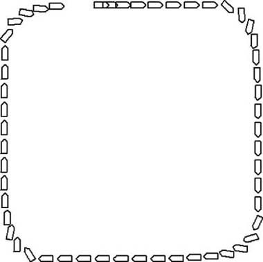
Figure 3-5 shows the zigzag pattern taken from the same example program. Again, notice the smooth turns. This gives the path a rather natural look. If this were an aircraft being simulated, one would also expect to see smooth turns.
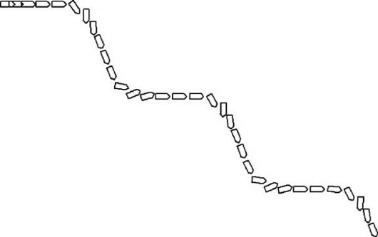
The pattern shown in Figure 3-6 consists of 10 instructions that tell the computer-controlled vehicle to go straight, turn 135 degrees right, go straight some more, turn 135 degrees left, and so on, until the pattern shown here is achieved.
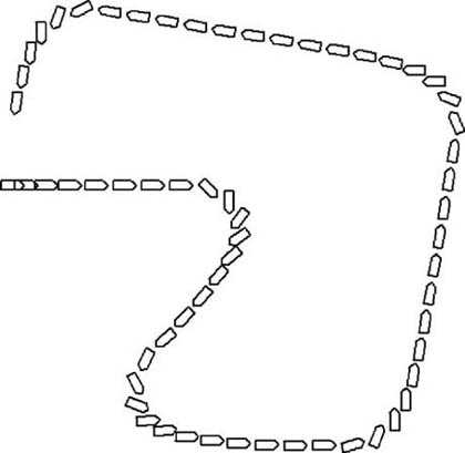
Just for fun, we included an arbitrary pattern in this example to show you that this algorithm does not restrict you to simple patterns such as squares and zigzags. You can encode any pattern you can imagine into a series of instructions in the same manner, enabling you to achieve seemingly intelligent movement.