
9. More Notebook Formatting
In This Chapter
• Adding color to text or the cell background
• Using color to highlight cells that meet specified criteria
• Working with gridlines
• Copying formatting from one cell to another
The last chapter introduced the basics of notebook formatting, and most of the techniques you learned focused on formatting that restructured your notebook. This chapter focuses on formatting that changes the appearance of your notebook to make it more attractive and easier to read. In this chapter, you’ll learn how to change fonts, use color, add borders and shadows to cells, and hide and display gridlines onscreen. Finally, I’ll show you how to copy formatting from one cell to another, which is a great timesaver because you don’t need to apply the same formatting multiple times.
Changing Fonts
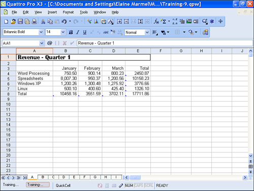
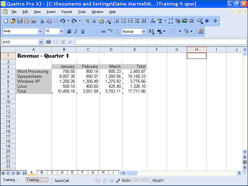
Changing fonts, particularly for spreadsheet titles or for headings, can make your spreadsheet more attractive and easier to read. For example, if you change the font of the spreadsheet title, you call attention to the title so that your reader immediately identifies the kind of information he or she is viewing. In Figure 9.1, you don’t immediately notice the spreadsheet title, but in Figure 9.2, the title jumps out at you.
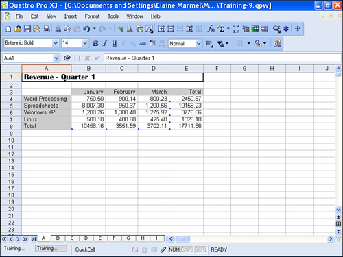
Figure 9.1. You don’t notice the spreadsheet title immediately in this spreadsheet.
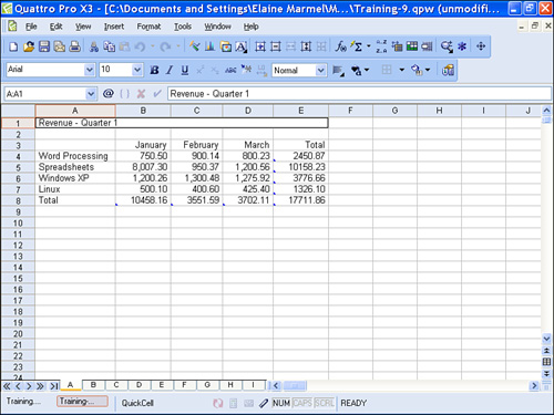
Figure 9.2. Because of the font difference, the spreadsheet title is immediately apparent.
To change fonts in a spreadsheet, follow these steps:
- Select the cell or cells for which you want to change fonts.
- Open the Font Face list and select the font you want to use (see Figure 9.3). Quattro Pro changes the cell’s font to the one you select.
Figure 9.3. Use these lists on the Property bar to change font face and size.
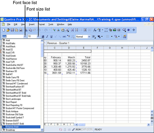
- Open the Font Size list and select the size for the font. Quattro Pro changes the font size of the selected cell(s).

Don’t get crazy changing fonts; too many different fonts on the same spreadsheet can make it harder to read, not easier. Limit the number of fonts on a spreadsheet to no more then three to maintain readability.
Using Color
Color can be another way you can enhance the readability and the appearance of a spreadsheet. In Quattro Pro, you can apply color to the text or values that appear in a cell or you can apply color to the background of a cell.
Although it may seem obvious, it’s important to note that color is effective only if your reader actually views the color, like on color printouts or on slides you create for a presentation.
Changing Text Color
Applying color to the text or values in a cell will call attention to that portion of the spreadsheet. To apply color to selected cells, follow these steps:
- Select the cell or cells to which you want to apply color to text or values.
- Open the Format menu and click Selection Properties. Quattro Pro displays the dialog box shown in Figure 9.4.
Figure 9.4. Use this dialog box to change the font of a cell or a selection of cells.
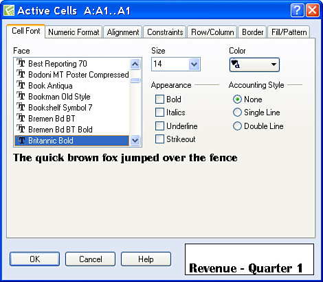
- Click the Cell Font tab.
- Click the Color button and select the color you want to apply to the selection. In the lower-right corner of the dialog box, Quattro Pro displays a sample of the cell using the color you applied.
- Click OK. Quattro Pro applies the color to the text or values in the selected cell(s).
Applying Color to Cell Backgrounds
Applying color to the background of cells is another technique you can use to enhance the appearance of your spreadsheet. In Figure 9.5, I’ve applied a light gray background to the cells that form the row and column headings for my data.
Figure 9.5. You can apply color to the background of a cell to enhance the appearance of your spreadsheet.
You’re probably wondering why you didn’t click the Background Color button. The Background Color button enables you to set the color of a pattern you might select from the pattern samples shown on the Fill/Pattern tab of the Active Cells dialog box. Although you can use patterns in the backgrounds of cells, be careful not to select a pattern that distracts from the readability of your spreadsheet.
To apply background color to cells, follow these steps:
- Select the cell or cells to which you want to apply background color.
- Open the Format menu and click Selection Properties. Quattro Pro displays the dialog box shown in Figure 9.6.
Figure 9.6. Select a background color for the cell using the Pattern Color button.
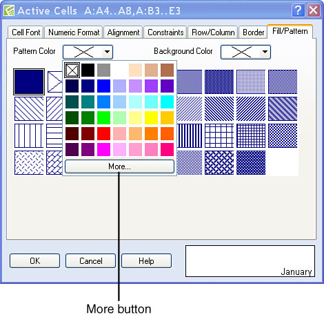
- Click the Fill/Pattern tab.
- Click the pattern you want to apply to the background of the cell; in this example, because I want to fill the entire background of the cell with color, but no pattern, I selected the pattern in the upper-left corner of the pattern choices.
- Click the Pattern Color button to select the color you want to apply to the selected cell(s). In the lower-right corner of the dialog box, Quattro Pro displays a sample of the cell(s) using the background color you selected.
- If you don’t see the color, click the More button. Quattro Pro displays the Select Color dialog box shown in Figure 9.7.
Figure 9.7. Use this dialog box to select a color variation.
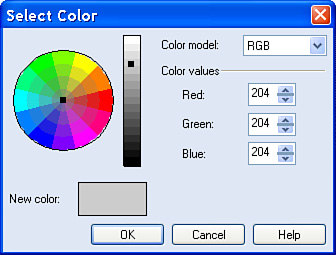
- Click the basic color in the color circle; then click in the list beside it to select the shade of the color you selected.
- Click OK. Quattro Pro redisplays the Fill/Pattern tab of the Active Cells dialog box.
- Click OK. Quattro Pro applies the color to the background of the selected cell(s).
Tip

From the Color model list, you can select RGB, HLS, or CMYK and then use the color value boxes to refine your selection even further. Using RGB, you set values for the amount of red, green, and blue in the color. Using HLS, you set the hue, luminosity, and saturation of the color. Using CMYK, you set the amount of cyan, magenta, and yellow in the color. Use whichever model makes you most comfortable.
Coloring Cells That Meet Certain Criteria
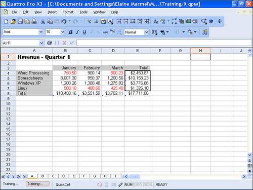
Here’s the situation: You want to call attention to some values in your spreadsheet but not others and you don’t want to manually apply color to the cells that meet your criteria. Further, the cells that meet your criteria either fall below or exceed a particular value. For example, in Figure 9.8, I’ve used the conditional coloring feature in Quattro Pro to display in red the values of the training classes for which revenue fell below $900.
Figure 9.8. When you conditionally color cells, Quattro Pro colors the values in cells that meet criteria you specify.
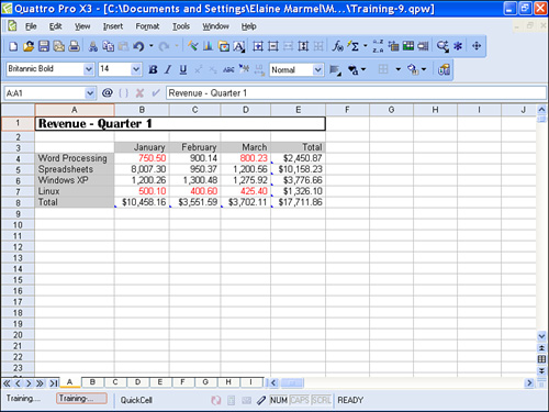
Because this book doesn’t show color, you can’t see the red, but if you examine the figure carefully, you’ll see that the values that meet the criteria—the ones that appear in red—appear lighter than the other values.
Follow these steps to use the Conditional Coloring feature in Quattro Pro:
- Open the Format menu and click Sheet Properties. Quattro Pro displays the Active Sheet dialog box shown in Figure 9.9.
Figure 9.9. Use this dialog box to set up the criteria Quattro Pro uses to color certain values in your spreadsheet.
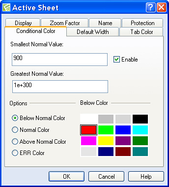
- Click the Conditional Color tab.
- In the Smallest Normal Value box, type the lowest value that Quattro Pro should not color. The smallest value you can specify is zero.
- In the Greatest Normal Value box, type the largest value Quattro Pro should not color. The largest value you can specify is 1e+300.
- In the Options section, select a color for each option. By default, Quattro Pro uses black for the Normal Color, red for the Below Normal Color and the ERR Color, and green for Above Normal Color.
- Click the Enable check box.
- Click OK. Quattro Pro applies colors to values in your spreadsheet according to the criteria you specified.
Adding Borders to Cells
Adding borders to cells is another way to draw attention to selected cells. And, although you can apply a colored border, using a black border can be particularly effective if color isn’t an option for you.
In Figure 9.10, I placed a black border around the totals for each training class.
Figure 9.10. You can use borders to call attention to selected cells.
To add borders to cells, follow these steps:
- Select the cell or cells around which you want to place borders.
- Open the Format menu and click Selection Properties. Quattro Pro displays the Active Cells dialog box.
- Click the Border tab.
- In the Segment Selection section, click the button that matches the type of border you want placed around the selected cells. In Figure 9.11, I clicked the Outline button.
Figure 9.11. Select the type of border you want to apply.
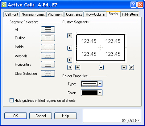
- In the Border Properties section, click the Type button to select the thickness of the border and click the Color button to select a color for the border.
- Click OK. Quattro Pro applies the border you selected to the cells you selected.
Hiding and Displaying Gridlines
By default, Quattro Pro displays vertical and horizontal gridlines onscreen. These gridlines don’t print unless you choose to print gridlines (see “Printing Gridlines” in Chapter 6, “Printing,” for details). But suppose that you intend to display your spreadsheet in a presentation you’re giving using an overhead projector and you really don’t want the gridlines to show. You can hide horizontal gridlines, vertical gridlines, or both by following these steps:
- Open the Format menu and click Sheet Properties. Quattro Pro displays the Active Sheet dialog box shown in Figure 9.12.
Figure 9.12. Use this dialog box to control the display of gridlines onscreen.
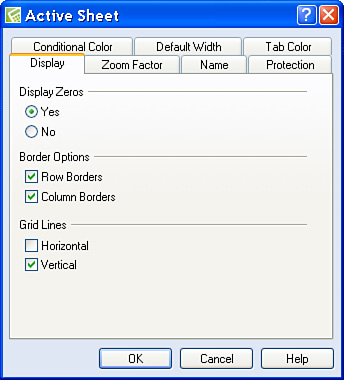
- Click the Display tab.
- Remove the checks from the Horizontal check box, the Vertical check box, or both.
- Click OK. Quattro Pro redisplays the spreadsheet with only the gridlines you specified. In Figure 9.13, I removed horizontal gridlines.
Figure 9.13. A spreadsheet with hidden horizontal gridlines.
Underlining Totals
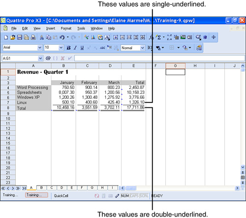
When your spreadsheet displays data that you sum to present totals, you may want to include the underline below the last number in the column you are totaling; you may also want to double-underline the total. In Quattro Pro, you can apply the appropriate accounting style to a selection, as I did in Figure 9.14.
Figure 9.14. Use Accounting Style to single-underline or double-underline values in a spreadsheet.
You can only apply one type of Accounting Style underlining to a selection. To apply single underlining to one selection and double underlining to a different selection, perform steps 1–5 twice.
To apply Accounting Style formatting, follow these steps:
- Select the cells to which you want to apply single underlining. In the sample spreadsheet shown in Figure 9.14, I selected B7.E7.
- Open the Format menu and click Selection Properties. Quattro Pro displays the Active Cells dialog box shown in Figure 9.15.
Figure 9.15. Use the options in the Accounting Style section to apply single or double underlining to the selected cells.
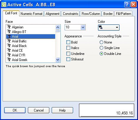
- Click the Cell Font tab.
- In the Accounting Style section, click the option appropriate for the type of underlining you want to apply.
- Click OK.
Copying Cell Formatting
The ability to copy cell formatting is one of my favorite timesaving techniques. You set up the formatting in one cell so that the cell looks just the way you want it to look. Then, you copy that formatting to any number of other cells.
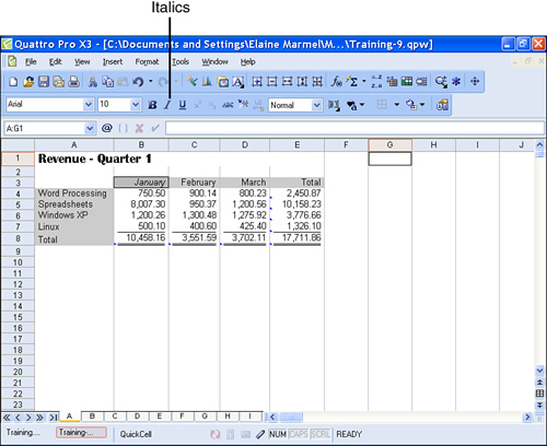
In Figure 9.16, I applied a slightly darker gray background to cell B3, used a light border, and then added italics by selecting the cell and clicking the Italics button on the Property bar.
Figure 9.16. Cell B3 looks the way I’d like cells C3.E3 to look.
I would like cells C3.E3 to look the way that cell B3 looks. I could manually apply the light gray background and the border to the cells the way I described earlier in this chapter in the sections, “Applying Color to Cell Backgrounds” and “Adding Borders to Cells,” and then I could apply italics to all the cells by clicking them and then clicking the Italics button.
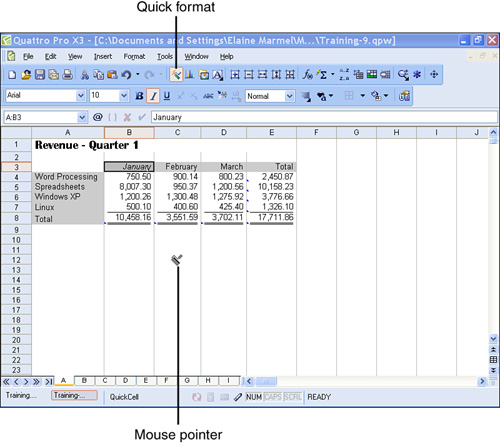
But it would be much faster to copy the formatting from B3 to the other cells. To copy formatting, select the cell that contains the formatting you want to apply and then click the QuickFormat button on the Notebook toolbar. Quattro Pro makes the button looks like it’s pressed in, and the mouse pointer shape changes to look like a roller you use to paint walls (see Figure 9.17). Behind the scenes, Quattro Pro “remembers” the formatting of the selected cell.
Figure 9.17. When you click the QuickFormat button, the mouse pointer shape changes to appear like a paint roller.
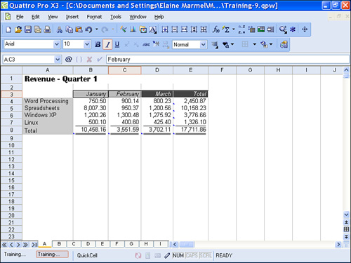
Click each cell to which you want to apply the formatting, or drag the mouse across the cells; Quattro Pro formats the cells you select to match the cell whose formatting you copied. In my example, I copied the formatting from B3 to C3.E3 (see Figure 9.18).
Figure 9.18. Quattro Pro copies the formatting of the cell you selected before clicking the QuickFormat button to the cells you select after clicking the QuickFormat button.
When you finish copying the formatting of the original cell, click the QuickFormat button to turn off the feature so that Quattro Pro doesn’t copy the formatting to every cell you click.