
Chapter 6. Queries That Select Records
In a typical database, with thousands or millions of records, you may find it quite a chore finding the information you need. In Chapter 3, you learned how to go on the hunt using the tools of the datasheet, including filtering, searching, and sorting. At first glance, these tools seem like the perfect solution for digging up bits of hard-to-find information. However, there’s a problem: The datasheet features are temporary.
To understand the problem, imagine you’re creating an Access database for a mail-order food company named Boutique Fudge. Using datasheet filtering, sorting, and column hiding, you can pare down the Orders table so it shows only the most expensive orders placed in the past month. (This information is perfect for targeting big spenders or crafting a hot marketing campaign.) Next, you can apply a different set of settings to find out which customers order more than five pounds of fudge every Sunday. (You could use this information for more detailed market research, or just pass it along to the Department of Health.) But every time you apply new datasheet settings, you lose your previous settings. If you want to jump back and forth from one view to another, you need to painstakingly reapply all your settings. If you’ve spent some time crafting the perfect view of your data, this process adds up to a lot of unnecessary extra work.
The solution to this problem is to use queries: readymade search routines that you store in your database. Even though the Boutique Fudge company has only one Orders table, it may have dozens (or more) queries, each with different sorting and filtering options. If you want to find the most expensive orders, you don’t need to apply the filtering, sorting, and column hiding settings by hand—instead, you can just fire up the MostExpensiveOrdersLastMonth query, which pulls out just the information you need. Similarly, if you want to find the fudge-aholics, you can run the LargeRepeatFudgeOrders query.
Queries are a staple of database design. In this chapter, you’ll learn all you need to design and fine-tune basic queries.
Query Basics
As the name suggests, queries are a way to ask questions about your data, like which products net the most cash, where do most customers live, and who ordered the monogrammed toothbrush? Access saves each query in your database, like it saves any other database object. Once you’ve saved a query, you can run it anytime you want to take a look at the live data that meets your criteria.
A query’s central ability is its amazing ability to reuse your hard work. Queries also introduce some new features that you don’t have with the datasheet alone:
Queries can combine related tables. This feature is insanely useful because it lets you craft searches that take related data into account. In the Boutique Fudge example, you can use this feature to create queries that find orders with specific product items or orders made by customers living in specific cities. Both these searches need relationships, because they branch out past the Orders table to take in information from other tables (like Products and Customers). You’ll see how this works on Joining Tables in a Query.
Queries can perform calculations. The Products table in the Boutique Fudge database lists price information, along with the quantity in stock. A query can multiply these details, and then add a column that lists the calculated value of the product you have on hand. You’ll try this trick in Chapter 7 (page 237).
Queries can perform summaries. To analyze large chunks of data, you can group together rows with similar information. You can group all the orders by customer to find out who is spending the most. Or you can group orders by products, to have a quick line-by-line list that compares the sales of Thermo-Nutcular Fudge against Vanilla Bean Dream. You’ll learn this technique in Chapter 8 (Grouping in a Totals Query).
Queries can automatically apply changes. If you want to find all the orders made by a specific person and reduce the cost of each one by 10 percent, a query can apply the entire batch of changes in one step. This action requires a different type of query, an action query, which you’ll consider in Chapter 9.
In this chapter, you’ll consider the simplest and most common type of query: the select query, which retrieves a subset of information from a table. Once you’ve retrieved this information, you can print or edit it using a datasheet, the same way you work with with a table.
Creating Queries
Access gives you three ways to create a query:
The query wizard gives you a quick-and-dirty way to build a simple query. However, this option also gives you the least control.
Design view offers the most common approach to query building. It provides a handy graphical tool that you can use to perfect any query.
SQL view gives you a behind-the-scenes look at the actual query command, which is a piece of text (ranging from one line to more than a dozen) that tells Access exactly what to do. The SQL view is where many Access experts hang out—and though it seems intimidating at first glance, it’s actually not that difficult to decipher (as you’ll see on Understanding the SQL View).
Creating a Query in Design View
The best starting point for query creation is the Design view. The following steps show you how it works. (To try this yourself, you can use the BoutiqueFudge.accdb database that’s included with the downloadable samples for this chapter.) The final result—a query that gets the results that fall in the first quarter of 2013—is shown in Figure 6-6.
Here’s what you need to do:
Choose Create→Queries→Query Design.
A new design window appears, where you can craft your query. But before you get started, Access pops open the Show Table window, where you can choose the tables that you want to work with (Figure 6-1).
Select the table that has the data you want, and then click Add (or just double-click the table).
In the Boutique Fudge example, you need the Orders table.
Access adds a box that represents the table to the design window. You can repeat this step to add several related tables, but for now stick with just one.
Click Close.
The Show Table dialog box disappears, giving you access to the Design view for the query.
Select the fields you want to include in your query.
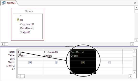
To select a field, double-click it in the table box (Figure 6-2). Take care not to add the same field more than once, or that column shows up twice in the results. If you’re using the Boutique Fudge example, make sure you choose at least the ID, DatePlaced, and CustomerID fields.
You can double-click the asterisk (*) to choose to include all the columns from a table. However, in most cases, it’s better to add each column separately. Not only does this help you more easily see at a glance what’s in your query, but it also lets you choose the column order and use the field for sorting and filtering.
Figure 6-2. Each time you double-click a field in the table box, Access adds it to the field list at the bottom of the window. You can then configure various settings to control filtering criteria and sorting for that column. If you don’t want to keep mousing back to the table box, you can add a field directly to the column list by choosing its name from the dropdown Field box.Arrange the fields from left to right in the order you want them to appear in the query results.
When you run the query, the columns appear in the same order as they’re listed in the column list in Design view. (Ordinarily, this system means the columns appear from left to right in the order you added them.) If you want to change the order, all you need to do is drag (as shown in Figure 6-3).
Figure 6-3. To reorder your columns, click the column header (the thin gray button at the top of the column), release the mouse button, and then drag the column to its new position. This technique is similar to the technique you use to arrange columns in the datasheet. In this example, the DatePlaced field is being moved to the far left side.If you want to hide one or more columns, clear the Show checkbox for those columns.
Ordinarily, Access shows every column you’ve added to the column list. However, in some situations you want to work with a column in your query, but not actually display its data. Usually, it’s because you want to use the column values for sorting or filtering.
Choose a sort order.
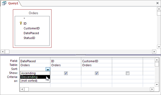
If you don’t supply a sort order, you’ll get the records right from the database in whatever order they happen to be. This convention usually (but not always) means the oldest records appear first, at the top of the table. To sort your table explicitly, choose the field you want to use to sort the results, and then, in the corresponding Sort box, choose a sorting option. In the current example, the table is sorted by date in descending order, so that the most recent orders are first in the list (Figure 6-4).
Set your filtering criteria.
Filtering (Filtering) is a tool that lets you focus on the records that interest you and ignore all the rest. Filtering cuts a large swath of data down to the information you need, and it’s the heart of many a query. (You’ll learn much more about building a filter expression in the next section.)
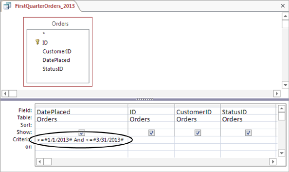
Once you have the filter expression you need, place it in the Criteria box for the appropriate field (Figure 6-5). In the current example, you can put this filter expression in the Criteria box for the DatePlaced field to get the orders placed in the first three months of the year:
>=#1/1/2013# And <=#3/31/2013#
You aren’t limited to a single filter—in fact, you can add a separate filter expression to each field. If you want to use a field for filtering but don’t want to display it in the results, then clear the Show checkbox for that field.
Figure 6-5. Here’s a filter that finds orders made in a date range (from January 1 to March 31, in the year 2013). Notice that when you use an actual hard-coded date as part of a condition (like January 1, 2013 in this example), Access brackets the date with # symbols. For a refresher about date syntax, refer to page 150.Choose Query Tools | Design→Results→Run.
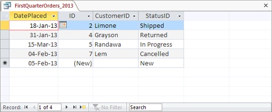
Now that you’ve finished the query, you’re ready to put it into action. When you run the query, you’ll see the results presented in a datasheet (complete with lookups on linked fields), just like when you edit a table. Figure 6-6 shows the result of the query on the Orders table.
You can switch back to Design view by right-clicking the tab title and then choosing Design View.
Figure 6-6. Here are the results of a query that shows orders placed within a specific date range. You can use the datasheet window to review or print your results, or you can edit information just as you would in a table datasheet.Note
The datasheet for your query acquires any formatting you applied to the datasheet of the underlying table. If you applied a hot-pink background and cursive font to the datasheet for the Orders table, the same settings apply to any queries that use the Orders table. However, you can change the datasheet formatting for your query just as you would with a table (see Datasheet Customization).
Save the query.
You can save your query anytime by using the keyboard shortcut Ctrl+S. If you don’t, Access automatically prompts you to save your query when you close the query tab (or your entire database). Of course, you don’t need to save your query. Sometimes you might create a query for a specific, one-time-only task. If you don’t plan to reuse the query, then there’s no point in cluttering up your database with extra objects.
The first time you save your query, Access asks for a name. Use the same naming rules that you follow for tables—refrain from using spaces or special characters, and capitalize the first letter in each word. A good query describes the view of data that it presents. One good choice for the example shown in Figure 6-6 is FirstQuarterOrders_2013.


Tip
Remember, when you save a query, you aren’t saving the query results—you’re just saving the query design, with all its settings. That way, you can run the query anytime to get the live results that match your criteria.
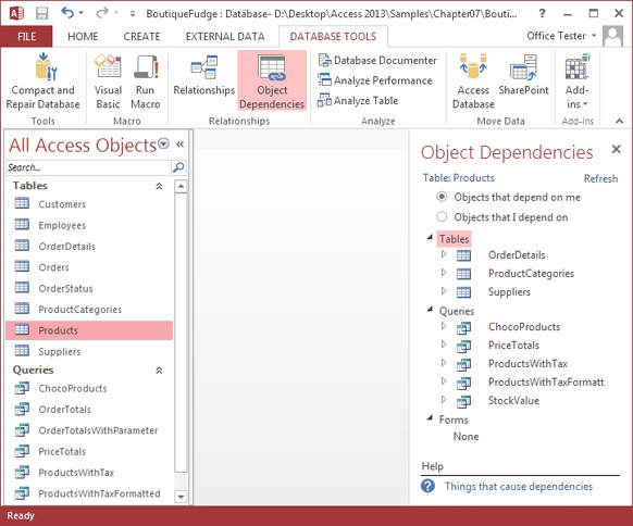
Once you’ve created a query, you’ll see it in your database’s navigation pane (Figure 6-7).

Tip
You can get this completed example, along with all the queries shown in this chapter, from the Missing CD page at www.missingmanuals.com/cds/access2013mm. Most of the queries, including FirstQuarterOrders_2013, are in the Boutique Fudge database.
You can launch the query anytime by double-clicking it. Suppose you’ve created a query named TopProducts that grabs all the expensive products in the Products table (using the filter criteria >50 on the Price field). Every time you need to review, print, or edit information about expensive products, you run the TopProducts query. To fine-tune the query settings, right-click the query in the navigation pane, and then choose Design View.
Access lets you open your table and any queries that use it at the same time; they all appear in separate tabs. However, you can’t modify the design of your table until you close all the queries that use it.
If you add new records to a table while a query is open, the new records don’t automatically appear in the query. Instead, you’ll need to run your query again. The quickest way is to choose Home→Records→Refresh→Refresh All. You can also close your query and open it again, or switch to Design view and then back to Datasheet view. Access runs your query every time it opens the Datasheet view.
Tip
Remember, a query is a view of some of the data in your table. If you edit some of the data in your query results, Access will change the corresponding records in the underlying table.
Building Filter Expressions
The secret to a good query is getting the information you want, and nothing more. To tell Access what records it should get (and which ones it should ignore), you need a filter expression.
The filter expression defines the records you’re interested in. If you want to find all the orders that were placed by a customer with the ID 1032, you could use this filter expression:
=1032
To put this filter expression into action, you need to put it in the Criteria box under the CustomerID field.
Technically, you could just write 1032 instead of =1032, but it’s better to stick to the second form, because that’s the pattern you’ll use for more advanced filter expressions. It starts with the operator (in this case, the equal sign) that defines how Access should compare the information, followed by the value (in this case, 1032) you want to use to make the comparison.
Note
If you’re using a multi-value field (Multi-Value Fields), Access includes the record in the query results if any value matches your filter. Imagine a Classes table that includes a multi-value InstructorID field (indicating that more than one teacher can team up to teach the same class). If you write the filter expression =1032 for the InstructorID field, Access includes any record where instructor 1032 teaches, whether or not other teachers are also assigned to the class.
Filter expressions are also called filter conditions—in fact, the two terms are interchangeable. This makes sense, because every filter sets out a condition that a record must match to be included in your results.
If filters seem uncannily familiar, there’s a reason. Filters have exactly the same syntax as the validation rules you used to protect a table from bad data (Validation Rules). The only difference is the way Access interprets the condition. A validation rule like <50 And >10 tells Access a value shouldn’t be allowed unless it falls in the desired range (10 to 50). But if you pop the same rule into a filter condition, it tells Access you aren’t interested in seeing the record unless it fits the range. Thanks to this similarity, you can use all the validation rules you saw earlier (starting on Writing a Field Validation Rule) as filter conditions.
Tip
In Chapter 7, you’ll learn how to beef up filter conditions with Access functions.
Getting the Top Records
If you’re matching text, you need to include quotation marks around your value. Otherwise, Access wonders where the text starts and stops.
="Harrington Red"
Instead of using an exact match, you can use a range. Add this filter expression to the OrderTotal field to find all the orders worth between $10 and $50:
<50 And >10
This filter expression actually contains two conditions (less than 50 and greater than 10), which are yoked together by the powerful And keyword. Alternatively, you can use the Or keyword if you want to see results that meet any one of the conditions you’ve included. (You can see examples of both on Combining Validation Conditions. In Chapter 7, you’ll consider some more powerful tools for crafting filter expressions.)
Date expressions are particularly useful. Just remember to bracket any hard-coded dates with the # character. If you add this filter condition to the DatePlaced field, it finds all the orders that were placed in 2013:
<#1/1/2014# And >#12/31/2012#
This expression works by requiring that dates are earlier than January 1, 2014, but later than December 31, 2012.
Note
With a little more work, you could craft a filter expression that gets the orders from the first 3 months of the current year, no matter what year it is. This trick requires the use of the functions Access provides for dates. You’ll see how to use them on Date Functions.
In some cases, filters are a bit more work than they should be. Suppose you want to see the 10 most expensive products. Using a filter condition, you can easily get the products that have prices above a certain threshold. Using sorting, you can arrange the results so the most expensive items turn up at the top. However, you can’t as easily tell Access to get just 10 records and then stop.
In this situation, the query Design view has a shortcut that can help you. Here’s how it works:
Open your query in Design view (or create a new query, and add the fields you want to use).
This example uses the Products table, and includes the ProductName and Price fields.
Sort your table so that the records you’re most interested in are at the top.
If you want to find the most expensive products, add a descending sort (Datasheet Navigation) on the Price field.
In the Query Tools | Design→Query Setup→Return box, choose a different option (Figure 6-8).
The standard option is All, which gets all the matching records. However, you can choose 5, 25, or 100 to get the top 5, 25, or 100 matching records, respectively. Or, you can use a percentage value like 25 percent to get the top quarter of matching records.
Figure 6-8. If you don’t see the number you want in the list, just type it into the Return box on your own. There’s no reason you can’t grab the top 27 most expensive products.Note
For the Query Tools | Design→Query Setup→Return box to work, you must choose the right sort order. To understand why, you need to know a little more about how this feature works. If you tell Access to get just five records, it actually performs the normal query, gets all the records, and arranges them according to your sort order. It then throws everything away except for the first five records in the list. If you’ve sorted your list so that the most expensive products are first (as in this example), you’re left with the top five budget-busting products in your results.
Run your query to see the results (Figure 6-9).


Creating a Simple Query with the Query Wizard
Design view is usually the best place to start constructing queries, but it’s not the only option. You can use the query wizard to give you an initial boost, and then refine your query in Design view.
The query wizard works by asking you a series of questions, and then creating the query that fits the bill. Unlike many of the other wizards in Access and other Office applications, the query wizard is relatively feeble. It’s a good starting point for query newbies, but not for an end-to-end performer.
Here’s how you can put the Query Wizard to work:
Choose Create→Queries→Query Wizard.
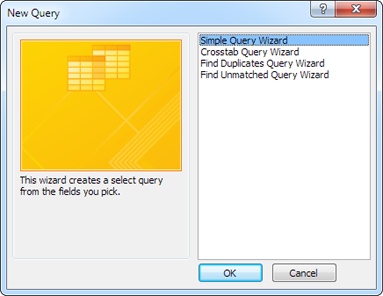
Access gives you a choice of several different wizards (Figure 6-10).
Choose a query type. The Simple Query Wizard is the best starting point for now.
The query wizard includes a few common kinds of queries. With the exception of the crosstab query, there’s nothing really unique about any of these choices. You’ll learn to create them all by using Design view:
Simple Query Wizard gets you started with an ordinary query, which displays a subset of data from a table. This query is the kind you created in the previous section.
Crosstab Query Wizard generates a crosstab query, which lets you summarize large amounts of data using different calculations. You’ll build one of your own on Crosstab Queries.
Find Duplicates Query Wizard is similar to the Simple Query Wizard, except it adds a filter expression that shows only records that share duplicated values. If you forgot to set a primary key or to create a unique index for your table, this option can help you clean up the mess.
Find Unmatched Query Wizard is similar to the Simple Query Wizard, except it adds a filter expression that finds unlinked records in related tables. You could use this to find an order that isn’t associated with any particular customer. You’ll learn how to find unmatched records on Finding Unmatched Records.
Click OK.
The first step of the query wizard appears.
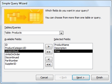
In the Tables/Queries box, choose the table that has the data you want. Then, add the fields you want to see in the query results, as shown in Figure 6-11.
For the best control, add the fields one at a time. Add them in the order you want them to appear from left to right in the query results.
You can add fields from more than one table. To do so, start by choosing one of the tables, add the fields you want, and then choose the second table and repeat the process. This process really makes sense only if the tables are related. You’ll learn more on Joining Tables in a Query.
Figure 6-11. To add a field, select it in the Available Fields list, and then click the > arrow button (or just double-click the field). You can add all fields at once by clicking the >> arrow button, and you can remove fields by selecting them in the Selected Fields list and then clicking <. In this example, three fields are included in the query.Click Next.
If your query includes a numeric field, the query wizard gives you the choice of creating a summary query that arranges rows into groups and that calculates information like totals and averages. You’ll learn about summary queries in Chapter 8. For now, if you get this choice, choose Detail and then click Next.
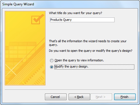
The final step of the query wizard appears (Figure 6-12).
Supply a query name in the “What title do you want for your query?” box.
If you want to fine-tune your query, choose “Modify the query design.” If you’re happy with what you’ve got, choose “Open the query to view information” to run the query.
One reason you may want to open your query in Design view is to add filter conditions (Building Filter Expressions) to pick out specific rows. Unfortunately, you can’t set filter conditions in the query wizard.
Your query opens in Design view or Datasheet view, depending on the choice you made in step 6. You can run it by choosing Query Tools | Design→Results→Run.
Understanding the SQL View
Behind the scenes, every query is actually a text command written in a specialized language called SQL (Structured Query Language). SQL is a staple of the database world, and it’s supported in all major database products, albeit with minor variations and idiosyncrasies.
Note
Database gurus still argue about whether SQL is pronounced “Es-Cue-El” (which is historically correct) or “Sequel” (which is how it’s used in the product name “Microsoft SQL Server”). In this book, we assume you’ll use the more hip “Sequel.”
As you craft a query in the design window (or using the query wizard), Access generates a matching SQL command. When you save your query, Access simply stores the text of this command in your database. That text is all Access needs to run the query later on.
Most of the time, you won’t spend much time contemplating the SQL that lurks under your queries’ surfaces. However, in some cases you may want to take a closer look. Here are some examples:
You want to perform an action that’s supported by SQL but isn’t available in the query designer. Of course, you’ll need to know more than a little about SQL to edit your command. Later in this chapter, you’ll see how to use SQL view to create a union query that combines the results from two similar tables.
You want to learn SQL. That’s a good skill to have if you’re planning a career as a database administrator, but it’s not really necessary if you’re sticking with Access.
You want to transplant a command into another type of database. Say you’re moving databases from Access to a high-powered Oracle database. This job is ambitious, and you’ll find that while you can move your data to its new home, you can’t move other database objects like queries. Instead, you need to take a closer look at the underlying SQL, which you can use to reconstruct the query in the new database.
You’re just plain curious. Looking at the SQL for your queries clears up a lot of the mystery behind how Access works.
You’re a SQL coding genius, and the query designer slows you down.
To take a look at the SQL command for a query, right-click the tab title, and then choose SQL view. Figure 6-13 shows what you see.

Analyzing a Query
Although SQL looks complex at first glance, all queries boil down to essentially the same ingredients. Consider the query for finding high-priced orders, which looks like this (with each line numbered for easy reference):
1 SELECT Products.ID, Products.ProductName, Products.Price
2 FROM Products
3 WHERE (((Products.Price)>50))
4 ORDER BY Products.Price;
Note
Sometimes, Access adds square brackets around field names. That means you might see Products. [ID] instead of Products.ID. Both variations are equivalent. However, you need the square brackets if your field name includes characters that have a specialized meaning in the SQL language, like the space. For example, if you have field called Product Name, the query must refer to it as Products.[Product Name] rather than Product. Product Name. Access always adds the square brackets when you need them, and it often adds them even when you don’t.
Here’s a breakdown of the first two lines:
Line 1 starts with the word SELECT, which indicates it’s a query that selects records (like all the queries you’ve seen in this chapter).
After the word SELECT is a comma-separated list of fields that you want to see. Each field is written out in the long format TableName.FieldName, just in case you decide to create a query that uses more than one table.
Line 2 starts with the word FROM, which indicates the table (or tables) that you’re searching. In this case, the Products table has the records you need.
These two lines represent a complete functioning query. However, you’ll often have more lines that apply filtering settings and sorting:
Line 3 starts with the word WHERE, which indicates the start of your filter conditions. In this case, there’s only one—a requirement that the product price be over $50. If you’ve defined more than one criteria on different fields, you see them all here, joined together using the AND operator.
Line 4 starts with the words “ORDER BY,” which define the sorting order. In this case, records are sorted from lowest to highest using the value in the Price field. In the case of a descending sort, you’d see the abbreviation “DESC” after the field name. If you’re sorting on multiple fields, you see a comma-separated field list.
The command ends with a final semicolon (;). Access doesn’t need this detail, but it’s a SQL-world convention.
The lesson is that every query you build is shaped out of a few common ingredients, represented by the SELECT, FROM, WHERE, and ORDER BY sections.
Access keeps all the different views of a query synchronized. If you make a change to the SQL text and then switch back to the Design view, you then see the newly modified version of the query (unless you’ve made a mistake, in which case Access delivers an error message).
To try it out, you can modify the SQL text so it selects an extra column and sorts on two fields, so products with the same price are arranged alphabetically (the new parts are highlighted in bold):
SELECT Products.ID, Products.ProductName, Products.Price,Products.DescriptionFROM Products WHERE (((Products.Price)>100)) ORDER BY Products.Price,Products.ProductName;
Right-click the tab title, and then choose Design View to see how these changes appear in the query designer.
Creating a Union Query
The query designer doesn’t recognize some rare SQL tricks. You can use them only by editing the SQL command in SQL view, and once you’ve made the change, you can’t look at your query in Design view any longer (unless you remove the unsupported change later on).
A union query merges the results from more than one table and then presents them in a single datasheet. This kind of query doesn’t fully work in the query designer, but that’s no reason you can’t use it.
Essentially, a union query is composed of two (or more) separate select queries. The trick is that the results from each select query must have the same structure. That means you need to retrieve similar columns from each table, in the same order. Assuming you can meet this standard, all you need to do is add the word “UNION” between the two queries.
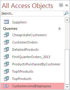
Here’s a union query that presents a list of names drawn from two tables—Customers and Employees:
SELECT Customers.FirstName, Customers.LastName
FROM Customers
UNION
SELECT Employees.FirstName, Employees.LastName
FROM Employees
This query works even though the structure of the Customers and Employees tables are different. The important part is that the query results from both tables—in this case, the FirstName and LastName fields—match up.
Note
You can create a union query even if the column names differ. In this example, that means that the query would still work if the columns in the Employees table were F_Name and L_Name. Access simply uses the column names from the first query when it displays the results in the datasheet.
In this example, when you view the query results, you see a list of customer names followed by a list of employee names, although you can’t necessarily tell where one table leaves off and the other begins. You also can’t edit any of the data—union queries are strictly for reviewing information, not changing it. Access doesn’t let you edit union queries in the query designer. If you right-click the tab title and then choose Design View, you wind up in SQL view instead.
Note
If there are any duplicates in the results, union queries show just one copy. You can change this behavior by replacing UNION with UNION ALL. In the previous example, this step causes a person who’s both an employee and a customer to show up twice in the combined results.
Access puts union queries in the Unrelated Objects section of the navigation pane and uses a different icon for them than for normal queries (Figure 6-14).
Union queries are a good way to link together similar tables that have been separated for reasons of performance, security, or distribution. (See the box on Approach One-to-One Relationships with Caution for the different reasons you might split a single set of data into different tables.) Union queries aren’t a good way to work with parent-child relationships. For this task you need join queries, which are described in the next section.
Queries and Related Tables
In Chapter 5, you learned how to split data into fundamental pieces and store it in distinct, well-organized tables. This sort of design’s only problem is that it’s more difficult to get the full picture when you have related data stored in separate places. Fortunately, Access has the perfect solution—you can bring the tables back together for display using a join.
A join is a query operation that pulls columns from two tables and fuses them together in one grid of results. You use joins to amplify child tables by adding information from the parent table. Here are some examples:
In the bobblehead database, you can show a list of bobblehead dolls (drawn from the child table Dolls) along with the manufacturer information for each doll (from the parent table Manufacturers).
In the Cacophoné music school database, you can get a list of available classes, with instructor information.
In the Boutique Fudge database, you can get a list of orders, complete with the details for the customer who placed the order.
Note
You’ve already learned how to create lookup tables to show just a bit of information from a linked table. A lookup can show the name of a product category in place of the ID number in the ProductID field. However, a join query is far more powerful. It can grab oodles of information from the linked table—far more than you could fit in a single field.
Figure 6-16 shows how a table join works.

Joining Tables in a Query
Access makes it remarkably easy to join two tables. The first step is adding both tables to your query, using the Show Table window. If you’re creating a new query in Design view, the Show Table window appears right away. If you’re working with a query you’ve already created, make sure you’re in Design view, right-click the window, and then choose Show Table.
Tip
You can add extra tables to a query without using the Show Table window. All you need to do is drag the table from the navigation pane and drop it on the query design surface.
If you’ve already defined a relationship between the two tables (using the Relationships window, as described on Defining a Relationship, or by creating a lookup, as described on Lookups with Related Tables), Access uses that relationship to automatically create a query join. You’ll see a line on the diagram that connects the appropriate fields, as shown in Figure 6-17.

If you add two unrelated tables, Access tries to help you out by guessing a relationship. If it spots a field with the same data type and the same name in both tables, it adds a join on this field. This action often isn’t what you want—for example, many tables share a common ID field. Also, if you’re following the database design rules from Six Principles of Database Design on page 89, your linked fields have slightly different names in each table, like ID and CustomerID. If you run into a problem where Access assumes a relationship that doesn’t exist, just remove the relationship before adding the join you really want.
If you haven’t already defined a relationship between the two related tables, you probably should, before you create your query (see Chapter 5 for full instructions). But if for some reason you’ve decided not to create the relationship (perhaps the database design was set in stone by another, less-savvy Access designer), you can manually define the join in the query window. To do so, just drag the linked field in one table to the matching field in the other table. You can also remove a join by right-clicking the line between the tables, and then choosing Delete.
Once you have your two tables in the query design window and you’ve defined the join, you’re ready to choose the fields you want. You can pick fields from both tables. You can also add filter conditions and supply a sort order, as you would with any other query. Figure 6-18 shows an example of a query that uses a join, and Figure 6-19 shows that same query in action.
Tip
When you have two linked tables, it’s easy to forget what you’re showing. If you join the Orders and Customers tables, and then select fields from each, what do you end up with: a list of customers or a list of orders? Easy—you get a list of orders, complete with customer information. Queries with linked tables always act on the child table and bring in additional information from the parent.


Note
When you perform a join, you see repeated information. If you join the Customers and Orders tables, you see the first and last name of a shopaholic customer appear next to several orders. However, this doesn’t violate the database rule against duplicate data. Even though the customer details appear in more than one place in the query results, they’re stored only once in the Customers table.
Remember, when you link a parent and child table with a join query, you’re really performing a query that gets all the records from the child table and then adds extra information from the parent table. For example, you can use a join query to get a list of orders (from the child table) and supplement each record with information about the customer that made the order. No matter how you create the join, you won’t ever get a list of customers with order information tacked on. That wouldn’t make sense, because every customer can make multiple orders.
Joins are one of the most useful features in any query writer’s toolkit. They let you display one table that has all the information you need.
Note
When using more than one table, there’s always a risk that two tables have a field with the same name. This possibility isn’t a problem if you don’t plan to show these fields in your query, but it can cause confusion if you do. One way to distinguish between the two fields is to rename one of them in the query datasheet. You’ll learn how to perform this trick with a calculated field on Calculated Fields.
Outer Joins
The queries you saw in the previous example use what database nerds call an inner join. Inner joins show only linked records—in other words, records that appear in both tables. If you perform a query on the Customers and Orders tables, you don’t see customers that haven’t placed an order. You also don’t see orders that aren’t linked to any particular customer (the CustomerID value’s blank) or aren’t linked to a valid record (they contain a CustomerID value that doesn’t match up to any record in the Customers table).
Outer joins are more accommodating—these joins include all the same results you’d see in an inner join, plus the leftover unlinked records from one of the two tables (it’s your choice which one). Obviously, these unlinked records show up in the query results with some blank values, which correspond to the missing information that the other table would supply.
Suppose you perform an outer join between the Orders and Customers tables, and then configure it so that all the order records are shown. Any orders that aren’t linked to a customer record have blank values in all the customer-related fields (like FirstName and LastName). In this example, there are two unlinked orders at the end of the listing:
FIRST NAME | LAST NAME | ID | DATE PLACED | STATUS ID |
Stanley | Lem | 7 | 13-Jun-2013 | Cancelled |
Toby | Grayson | 4 | 03-Nov-2012 | |
Toby | Grayson | 6 | 03-Nov-2012 | Shipped |
18 | 01-Jan-2011 | In Progress | ||
19 | 01-Jan-2011 | In Progress |
In this particular example, it doesn’t make sense for orders that aren’t linked to a customer to exist. In fact, it probably indicates an order that was entered incorrectly. However, if you suspect a problem, an outer join can help you track down the problem.
Tip
You can prevent orphaned order records altogether by making CustomerID a required value (Data Integrity Basics) and enforcing referential integrity (Defining a Relationship).
You can also perform an outer join between the Orders and Customers tables that shows all the customer records. In this case, at the end of the query results, you’ll see every unlinked customer record, with the corresponding order fields left blank:
FIRST NAME | LAST NAME | ID | DATE PLACED | STATUS ID |
Stanley | Lem | 7 | 13-Jun-2013 | Cancelled |
Toby | Grayson | 4 | 03-Nov-2012 | Returned |
Toby | Grayson | 6 | 03-Nov-2012 | Shipped |
Ben | Samatara | |||
Goosey | Mason | |||
Tabasoum | Khan |
In this case, the outer join query picks up three stragglers.
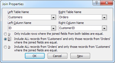
So how do you add an outer join to your query? You start with an inner join (which Access usually adds automatically), and then convert it to an outer join. To do so, just right-click the join line that links the two tables in the design window, and then choose Join Properties (or just double-click the line). The Join Properties window (Figure 6-20) appears and lets you change the type of join you’re using.
Finding Unmatched Records
Inner joins are by far the most common joins. However, outer joins let you create at least one valuable type of query: a query that can track down unmatched records.
You’ve already seen how an outer join lets you see a list of all your orders, plus the customers that haven’t made any orders. That combination isn’t terribly useful. But with a little fine-tuning, you can filter out the real customers and create a list with only those people who haven’t bought anything. The marketing department is already salivating over this technique, which could help them target potential customers for a first-time-buyer promotion.
To craft this query, you start with the outer-join query that includes all the customer records. Then, you simply add one more ingredient: a filter condition that matches records that don’t have an order ID. Technically, these are considered null (empty) values.
Here’s the filter condition you need, which you must place in the Criteria box for the ID field of the Orders table:
Is Null
Now, when Access performs the query, it includes only the customer records that aren’t linked to anything in the Orders table. Figure 6-21 shows the query in Design view.

Multiple Joins
Just as you’re getting comfortable with inner and outer joins, Access has another feature to throw your way. Many queries don’t stop at a single join. Instead, they use three, four, or more to bring multiple related tables into the mix.
Although this sounds complicated at first, it really isn’t. Multiple joins are simply ways of bringing more related information into your query. Each join works the same in a multiple-join situation as it does when you use it on its own. To use multiple joins, just add all the tables you want from the Show Table window, make sure the join lines appear, and then choose the fields you want. Access is almost always intelligent enough to figure out what you’re trying to do.
Figure 6-22 shows an example where a child table has two parents that can both contribute some extra information.

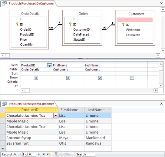
Sometimes, the information you want is more than one table away. Consider the OrderDetails table Boutique Fudge uses to list each item in a customer’s order. On its own, the OrderDetails table doesn’t provide a link to the customer who ordered the item, but it does provide a link to the related order record. (See Ordering Products for a discussion of this design.) If you want to get the information about who ordered each item, you need to add the OrderDetails, Orders, and Customers tables to your query, as shown in Figure 6-23.
Multiple joins are also the ticket if you have a many-to-many relationship with a junction table (Many-to-Many Relationship), like the one between teachers and classes. As you’ll remember from Chapter 5 (Identifying the Tables), the Cacophoné Studios music school uses an intermediary table to track teacher class assignment. If you want to get a list of classes, complete with instructor names, you need to create a query with three tables: Classes, Teachers, and Teachers_Classes (see Figure 6-24).
