
Texture Mapping Techniques
Texture mapping is a powerful building block of graphics techniques. It is used in a wide range of applications, and is central to many of the techniques used in this book. The basics of texture mapping have already been covered in Chapter 5 and serves as a background reference for texture-related techniques.
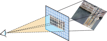
The traditional use of texture mapping applies images to geometric surfaces. In this chapter we’ll go further, exploring the use of texture mapping as an elemental tool and building block for graphics effects. The techniques shown here improve on basic texture mapping in two ways. First, we show how to get the most out of OpenGL’s native texturing support, presenting techniques that allow the application to maximize basic texture mapping functionality. Examples of this include rendering very large textures using texture paging, prefiltering textures to improve quality, and using image mosaics (or atlases) to improve texture performance.
We also re-examine the uses of texture mapping, looking at texture coordinate generation, sampling, and filtering as building blocks of functionality, rather than just a way of painting color bitmaps onto polygons. Examples of these techniques include texture animation, billboards, texture color coding, and image warping. We limit our scope to the more fundamental techniques, focusing on the ones that have potential to be used to build complex approaches. More specialized texturing techniques are covered in the chapters where they are used. For example, texture mapping used in lighting is covered in Chapter 15. Volumetric texturing, a technique for visualizing 3D datasets, is presented in Section 20.5.8.
14.1 Loading Texture Images into a Framebuffer
Although there is no direct OpenGL support for it, it is easy to copy an image from a texture map into the framebuffer. It can be done by drawing a rectangle of the desired size into the framebuffer, applying a texture containing the desired texture image. The rectangle’s texture coordinates are chosen to provide a one-to-one mapping between texels and pixels. One side effect of this method is that the depth values of the textured image will be changed to the depth values of the textured polygon. If this is undesirable, the textured image can be written back into the framebuffer without disturbing existing depth buffer values by disabling depth buffer updates when rendering the textured rectangle. Leaving the depth buffer intact is very useful if more objects need to be rendered into the scene with depth testing after the texture image has been copied into the color buffer.
The concept of transferring images back and forth between a framebuffer and texture map is a useful building block. Writing an image from texture memory to the framebuffer is often faster than transferring it from system memory using glDrawPixels. If an image must be transferred to the framebuffer more than once, using a texture can be the high-performance path. The texture technique is also very general, and can be easily extended. For example, when writing an image back into the framebuffer with a textured polygon, the texture coordinates can be set to arbitrarily distort the resulting image. The distorted image could be the final desired result, or it could be transferred back into the texture, providing a method for creating textures with arbitrarily warped images.
14.2 Optimizing Texture Coordinate Assignment
Rather than using it to create special effects, in some cases distorting a texture image can be used to improve quality. Sloan et al. (1997) have explored optimizing the assignment of texture coordinates based on an “importance map” that can encode both intrinsic texture properties as well as user-guided highlights. This approach highlights the fact that texture images can have separate “interesting” regions in them. These can be areas of high contrast, fine detail, or otherwise draw the viewer’s attention based on its content. A simple example is a light map containing a region of high contrast and detail near the light source with the rest of the texture containing a slowly changing, low-contrast image.
A common object modeling approach is to choose and position vertices to represent an object accurately, while maintaining a “vertex budget” constraint to manage geometry size and load bandwidth. As a separate step, the surface is parameterized with texture coordinates so surface textures can be applied. Adding the notion of textures with regions of varying importance can lead to changes in this approach.
The first step is to distort a high-resolution version of the texture image so the regions of interest remain large but the remainder shrinks. The resulting texture image is smaller than the original, which had high-image resolution everywhere, even where it wasn’t needed. The technique described in Section 5.3 can be used to generate the new image. The parameterization of the geometry is also altered, mapping the texture onto the surface so that the high and low importance regions aren’t distorted, but instead vary in texel resolution. This concept is shown in Figure 14.1.
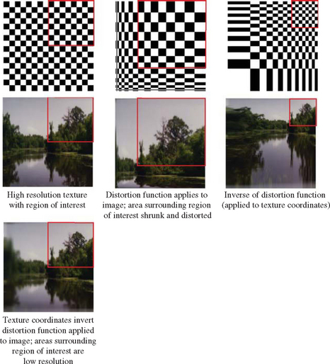
To do this properly both the texture, with its regions of high and low interest, and the geometry it is applied to must be considered. The tessellation of the model may have to be changed to ensure a smooth transition between high- and low-resolution regions of the texture. At least two rows of vertices are needed to transition between a high-resolution scaling to a low-resolution one; more are needed if the transition region requires fine control.
The idea of warping the texture image and altering the texture coordinate assignment can be thought of as a general approach for improving texture appearance without increasing texture size. If the OpenGL implementation supports multitexturing, a single texture can be segmented into multiple textures with distinct low and high interest regions.
14.3 3D Textures
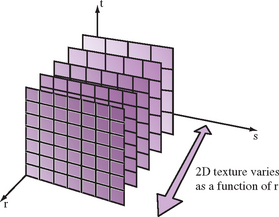
The classic application of 3D texture maps is to to use them to represent the visual appearance of a solid material. One example would be to procedurally generate a solid representation of marble, then apply it to an object, so that the object appears to be carved out of the stone. Although this 3D extension of the surface mapping application is certainly valuable, 3D texture maps can do more. Put in a more general context, 3D textures can be thought of as a 2D texture map that varies as a function of its r coordinate value. Since the 3D texture filters in three dimensions, changing the r value smoothly will linearly blend from one 2D texture image slice to the next (Figure 14.2). This technique can be used to create animated 2D textures and is described in more detail in Section 14.12.
Two caveats should be considered when filtering a 3D texture. First, OpenGL doesn’t make any distinction between dimensions when filtering; if GL_LINEAR filtering is chosen, both the texels in the r direction, and the ones in the s and t directions, will be linearly filtered. For example, if the application uses nearest filtering to choose a specific slice, the resulting image can’t be linearly filtered. This lack of distinction between dimensions also leads to the second caveat. When filtering, OpenGL will choose to minify or magnify isotropically based on the size ratio between texel and pixel in all dimensions. It’s not possible to stretch an image slice and expect minification filtering to be used for sampling in the r direction.
The safest course of action is to set GL_TEXTURE_MIN_FILTER and GL_TEXTURE_MAG_FILTER to the same values. It is also prudent to use GL_LINEAR instead of GL_NEAREST. If a single texture slice should be used, compute r to index exactly to it: the OpenGL specification is specific enough that the proper r value is computable, given the texture dimensions. Finally, note that using r for the temporal direction in a 3D texture is arbitrary; OpenGL makes no distinction, the results depend solely on the configuration set by the application.
3D textures can also be parameterized to create a more elaborate type of billboard. A common billboard technique uses a 2D texture applied to a polygon that is oriented to always face the viewer. Billboards of objects such as trees behave poorly when the object is viewed from above. A 3D texture billboard can change the textured image as a function of viewer elevation angle, blending a sequence of images between side view and top view, depending on the viewer’s position.
If the object isn’t seen from above, but the view around the object must be made more realistic, a 3D texture can be composed of 2D images taken around the object. An object, real or synthetic, can be imaged from viewpoints taken at evenly spaced locations along a circle surrounding it. The billboard can be textured with the 3D texture, and the r coordinate can be selected as a function of viewer position. This sort of “azimuth billboard” will show parallax motion cues as the view moves around the billboard, making it appear that the billboard object has different sides that come into view. This technique also allows a billboard to represent an object that isn’t as cylindrically symmetric about its vertical access.
This technique has limits, as changes in perspective are created by fading between still images taken at different angles. The number of views must be chosen to minimize the differences between adjacent images, or the object itself may need to be simplified. Using a billboard of any variety works best if the object being billboarded isn’t the focus of the viewer’s attention. The shortcuts taken to make a billboard aren’t as noticeable if billboards are only used for background objects.
The most general use of 3D textures is to represent a 3D function. Like the 2D version, each texel stores the result of evaluating a function with a particular set of parameter values. It can be useful to process the s, t, and r values before they index the texture, to better represent the function. This processing can be done with texgen or a texture transform matrix functionality. As with the previous two methods, using GL_LINEAR makes it possible to interpolate between arbitrary sample points. A non-linear function is often approximately linear between two values, if the function values are sampled at close enough intervals.
14.4 Texture Mosaics
Many complex scenes have a large number of “odds and ends” textures. These low-resolution textures are used to add diversity and realism to the scene’s appearance. Additionally, many small textures are often needed for multipass and multitexture surfaces, to create light maps, reflectance maps, and so forth. These “surface realism” textures are often low resolution; their pattern may be replicated over the surface to add small details, or stretched across a large area to create a slowly changing surface variation.
Supporting such complex scenes can be expensive, since rendering many small, irregularly sized textures requires many texture binds per scene. In many OpenGL implementations the cost of binding a texture object (making it the currently active texture) is relatively high, limiting rendering performance when a large number of textures are being used in each rendered frame. If the implementation supports multitexturing, the binding and unbinding of each texture unit can also incur a high overhead.
Beyond binding performance, there are also space issues to consider. Most implementations restrict texture map sizes to be powers of two to support efficient addressing of texels in pipeline implementations. There are extensions that generalize the addressing allowing non-power-of-two sizes, such as ARB_texture_non_power_of_two and EXT_texture_rectangle. Nevertheless, to meet a power-of-two restriction, small texture images may have to be embedded in a larger texture map, surrounded by a large boundary. This is wasteful of texture memory, a limited resource in most implementations. It also makes it more likely that fewer textures in the scene fit into texture memory simultaneously, forcing the implementation to swap textures in and out of the graphics hardware’s texture memory, further reducing performance.
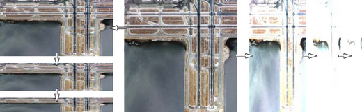
Both the texture binding and space overhead of many small textured images can be reduced by using a technique called texture mosaicing (or sometimes texture atlasing) (Figure 14.3). In this technique, many small texture images are packed together into a single texture map. Binding this texture map makes all of its texture images available for rendering, reducing the number of texture binds needed. In addition, less texture memory is wasted, since many small textures can be packed together to form an image close to power-of-two dimensions.
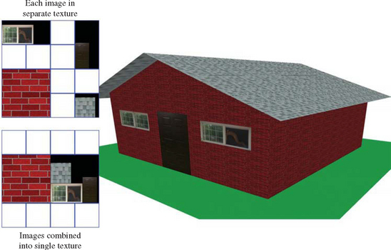
Texture mosaicing can also be used to reduce the overhead of texture environment changes. Since each texture often has a specific texture environment associated with it, a mosaic can combine images that use the same texture environment. When the texture is made current, the texture environment can be held constant while multiple images within the texture map are used sequentially. This combining of similar texture images into a single texture map can also be used to group textures that will be used together on an object, helping to reduce texture binding overhead.
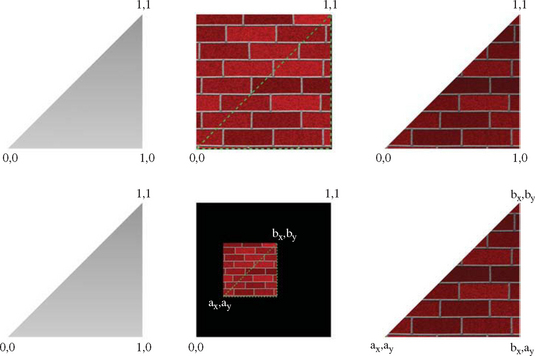
The individual images in the mosaic must be separated enough so that they do not interfere with each other during filtering. If two images are textured using nearest filtering, then they can be adjacent, but linear filtering requires a one-pixel border around each texture, so the adjacent texture images do not overlap when sampled near their shared boundaries.
Mosaicing mipmapped textures requires greater separation between images. If a series of mipmap layers contain multiple images, then each image must be enclosed in a power-of-two region, even if the image doesn’t have a power-of-two resolution. This avoids sampling of adjacent images when coarse mipmap levels are used. This space-wasting problem can be mitigated somewhat if only a subset of the mipmap levels (LODs) are needed. OpenGL 1.2 supports texture LOD clamping which constrains which LODs are used and therefore which levels need to be present. Blending of coarse images also may not be a problem if the adjacent textures are chosen so that their coarser layers are very similar in appearance. In that case, the blending of adjacent images may not be objectionable.
A primitive textured using mosaiced textures must have its texture coordinates modified to access the proper region of the mosaic texture map. Texture coordinates for an unmosaiced texture image will expect the texture image to range from 0 to 1. These values need to be scaled and biased to match the location of desired image in the mosaic map (Figure 14.4). The scaled and biased texture coordinates can be computed once, when the objects in the scene are modeled and the mosaiced textures created, or dynamically, by using OpenGL’s texgen or texture matrix functions to transform the texture coordinates as the primitives are rendered. It is usually better to set the coordinates at modeling time, freeing texgen for use in other dynamic effects.
14.5 Texture Tiling
There is an upper limit to the size of a texture map that an implementation can support. This can make it difficult to define and use a very large texture as part of rendering a high-resolution image. Such images may be needed on very high-resolution displays or for generating an image for printing. Texture tiling provides a way of working around this limitation. An arbitrarily large texture image can be broken up into a rectangular grid of tiles. A tile size is chosen that is supported by the OpenGL implementation. This texture tiling method is related to texture paging, described in Section 14.6.
OpenGL supports texture tiling with a number of features. One is the strict specification of the texture minification filters. On conformant implementations, this filtering is predictable, and can be used to seamlessly texture primitives applied one at a time to adjacent regions of the textured surface.
To apply a texture to these regions, a very large texture is divided into multiple tiles. The texture tiles are then loaded and used to texture in several passes. For example, if a 1024 × 1024 texture is broken up into four 512 × 512 images, the four images correspond to the texture coordinate ranges ![]() and
and ![]() .
.
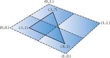
As each tile is loaded, only the portions of the geometry that correspond to the appropriate texture coordinate ranges for a given tile should be drawn. To render a single triangle whose texture coordinates are (0.1, 0.1), (0.1, 0.7), and (0.8, 0.8), the triangle must be clipped against each of the four tile regions in turn. Only the clipped portion of the triangle—the part that intersects a given texture tile—is rendered, as shown in Figure 14.5. As each piece is rendered, the original texture coordinates must be adjusted to match the scaled and translated texture space represented by the tile. This transformation is performed by loading the appropriate scale and translation onto the texture matrix.
Normally clipping the geometry to the texture tiles is performed as part of the modeling step. This can be done when the relationship between the texture and geometry is known in advance. However, sometimes this relationship isn’t known, such as when a tiled texture is applied to arbitrary geometry. OpenGL does not provide direct support for clipping the geometry to the tile. The clipping problem can be simplified, however, if the geometry is modeled with tiling in mind. For a trivial example, consider a textured primitive made up of quads, each covered with an aligned texture tile. In this case, the clipping operation is easy. In the general case, of course, clipping arbitrary geometry to the texture tile boundaries can involve substantially more work.
One approach that can simplify the clipping stage of texture tiling is to use stenciling (Section 6.2.3) and transparency mapping (Section 11.9.2) to trim geometry to a texture tile boundary. Geometry clipping becomes unnecessary, or can be limited to culling geometry that doesn’t intersect a given texture tile to improve performance. The central idea is to create a stencil mask that segments the polygons that is covered by a given texture tile from the polygons that aren’t. The geometry can be rendered with the proper tile texture applied, and the stencil buffer can be set as a side effect of rendering it. The resulting stencil values can be used in a second pass to only render the geometry where it is textured with the tile (Figure 14.6).
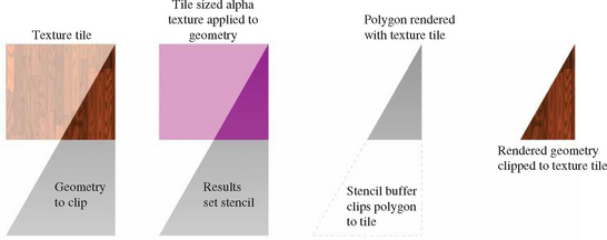
Creating the stencil mask itself can be done by using a “masking” texture. This texture sets an alpha value only where it’s applied to the primitive. Alpha test can then be used to discard anything not drawn with that alpha value (see Section 6.2.2). The undiscarded fragments can then be used with the proper settings of stencil test and stencil operation to create a stencil mask of the region being textured. Disabling color and depth buffer updates, or setting the depth test to always fail will ensure that only the stencil buffer is updated.
One area that requires care is clamping. Since the tiling scenario requires applying a masking texture that only covers part of the primitive, what happens outside the texture coordinate range of [0, 1] must be considered. One approach is to configure the masking texture to use the GL_CLAMP_TO_BORDER wrap mode, so all of the geometry beyond the applied texture will be set to the border color. Using a border color with zero components (the default) will ensure that the geometry not covered by the texture will have a different alpha value.
Here is a procedure that puts all of these ideas together:
1. Create a texture of internal type GL_ALPHA. It can have a single texel if desired.
2. Set the parameters so that GL_NEAREST filtering is used, and set the wrap mode appropriately.
3. Set the texture environment to GL_REPLACE.
4. Apply the texture using the same coordinate, texgen, and texture transform matrix settings that will be used in the actual texture tile.
5. Enable and set alpha testing to discard all pixels that don’t have an alpha value matching the masking texture.
6. Set up the stencil test to set stencil when the alpha value is correct.
7. Render the primitive with the masking texture applied. Disable writes to the color and depth buffer if they should remain unchanged.
8. Re-render the geometry with the actual tiled texture, using the new stencil mask to prevent any geometry other than the tiled part from being rendered.
If the tiled textures are applied using nearest filtering, the procedure is complete. In the more common case of linear or mipmap filtered textures, there is additional work to do. Linear filtering can generate artifacts where the texture tiles meet. This occurs because a texture coordinate can sample beyond the edge of the texture. The simple solution to this problem is to configure a one-texel border on each texture tile. The border texels should be copied from the adjacent edges of the neighboring tiles.
A texture border ensures that a texture tile which samples beyond its edges will sample from its neighbors texels, creating seamless boundaries between tiles. Note that borders are only needed for linear or mipmap filtering. Clamp-to-edge filtering can also be used instead of texture borders, but will produce lower quality results. See Section 5.1.1 for more information on texture borders.
14.6 Texture Paging
As applications simulate higher levels of realism, the amount of texture memory they require can increase dramatically. Texture memory is a limited, expensive resource, so directly loading a high-resolution texture is not always feasible. Applications are often forced to resample their images at a lower resolution to make them fit in texture memory,with a corresponding loss of realism and image quality. If an application must view the entire textured image at high resolution, this, or a texture tiling approach (as described in Section 14.5) may be the only option.
But many applications have texture requirements that can be structured so that only a small area of large texture has to be shown at full resolution. Consider a flight simulation example. The terrain may be modeled as a single large triangle mesh, with texture coordinates to map it to a single, very large texture map, possibly a mipmap. Although the geometry and the texture are large, only terrain close to the viewer is visible in high detail. Terrain far from the viewer must be textured using low-resolution texture levels to avoid aliasing, since a pixel corresponding to these areas covers many texels at once. For similar reasons, many applications that use large texture maps find that the maximum amount of texture memory in use for any given viewpoint is bounded.
Applications can take advantage of these constraints through a technique called texture paging. Rather than loading complete levels of a large image, only the portion of the image closest to the viewer is kept in texture memory. The rest of the image is stored in system memory or on disk. As the viewer moves, the contents of texture memory are updated to keep the closest portion of the image loaded.
Two different approaches can be used to implement this technique. The first is to use a form of texture tiling. The texture is subdivided into fixed sized tiles. Textured geometry is matched up with the tiles that cover it, and segmented to match the tile boundaries. This segmentation can happen when the geometry is modeled, by re-tessellating it into tile-sized pieces (with its texture coordinates changed to map the tile properly) or it can be done at runtime through clipping combined with texgen or the texture transform matrix.
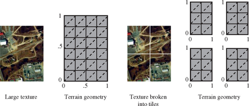
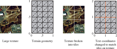
When tiled geometry is rendered, it is rendered one tile at a time, with texture coordinates set appropriately to apply the tile to the surface. Texture memory is reloaded when a new tile is needed. For geometry that is farther from the viewer, tiles containing lower resolution texture levels are used to avoid aliasing artifacts. Figure 14.7 shows a texture broken up into tiles, and its geometry tessellated and texture coordinates changed to match.
The tiling technique is conceptually straightforward, and is used in some form by nearly all applications that need to apply a large texture to geometry (see Section 14.5). There are some drawbacks to using a pure tiling approach, however. The part of the technique that requires segmenting geometry to texture tiles is the most problematic. Segmenting geometry requires re-tessellating it to match tile boundaries, or using techniques to clip it against the current tile. In addition, the geometry’s texture coordinates must be adjusted to properly map the texture tile to the geometry segment.
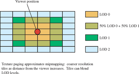
For linear filtering, tile boundaries can be made invisible by carefully clipping or tessellating the geometry so that the texture coordinates are kept within the tile’s [0.0, 1.0] range, and using texture borders containing a strip of texels from each adjacent tile (see Section 5.1.1 for more details on texture borders). This ensures that the geometry is textured properly across the edge of each tile, making the transition seamless. A clean solution is more elusive when dealing with the boundary between tiles of different texture resolution, however. One approach is to blend the two resolutions at boundary tiles, using OpenGL’s blend functionality or multitexturing. Figure 14.8 shows how tiles of different resolution are used to approximate mipmapping, and how tiles on each LOD boundary can be blended. Alternatively, linear filtering with mipmapping handles the border edges, at the expense of loading a full mipmap pyramid rather than a single level.
The process of clipping or re-tessellating dynamic geometry to match each image tile itself is not always easy. An example of dynamic geometry common to visual simulation applications is dynamic terrain tessellation. Terrain close to the viewer is replaced with more highly tessellated geometry to increase detail, while geometry far from the viewer is tessellated more coarsely to improve rendering performance. In general, forcing a correspondence between texture and geometry beyond what is established by texture coordinates should be avoided, since it increases complication and adds new visual quality issues that the application has to cope with.
Given sufficient texture memory, geometry segmentation can be avoided by combining texture tiles into a larger texture region, and applying it to the currently visible geometry. Although it uses more texture memory, the entire texture doesn’t need to be loaded, only the region affecting visible geometry. Clipping and tessellation is avoided because the view frustum itself does the clipping. To avoid explicitly changing the geometry’s texture coordinates, the texture transform matrix can be used to map the texture coordinates to the current texture region.
To allow the viewer to move relative to the textured geometry, the texture memory region must be updated. As the viewer moves, both the geometry and the texture can be thought of as scrolling to display the region closest to the viewer. In order to make the updates happen quickly, the entire texture can be stored in system memory, then used to update the texture memory when the viewer moves.
Consider a single level texture. Define a viewing frustum that limits the amount of visible geometry to a small area,—small enough that the visible geometry can be easily textured. Now imagine that the entire texture image is stored in system memory. As the viewer moves, the image in texture memory can be updated so that it exactly corresponds to the geometry visible in the viewing frustum:
1. Given the current view frustum, compute the visible geometry.
2. Set the texture transform matrix to map the visible texture coordinates into 0 to 1 in s and t.
3. Use glTexImage2D to load texture memory with the appropriate texel data, using GL_SKIP_PIXELS and GL_SKIP_ROWS to index to the proper subregion.
This technique remaps the texture coordinates of the visible geometry to match texture memory, then loads the matching system memory image into texture memory using glTexImage2D.
14.6.1 Texture Subimage Loading
While the technique described previously works, it is a very inefficient use of texture load bandwidth. Even if the viewer moves a small amount, the entire texture level must be reloaded to account for the shift in texture. Performance can be improved by loading only the part of the texture that’s newly visible, and somehow shifting the rest.
Shifting the texture can be accomplished by taking advantage of texture coordinate wrapping (also called torroidal mapping). Instead of completely reloading the contents of texture memory, the section that has gone out of view from the last frame is loaded with the portion of the image that has just come into view with this frame. This technique works because texture coordinate wrapping makes it possible to create a single, seamless texture, connected at opposite sides. When GL_TEXTURE_WRAP_S and GL_TEXTURE_WRAP_T are set to GL_REPEAT (the default), the integer part of texture coordinates are discarded when mapping into texture memory. In effect, texture coordinates that go off the edge of texture memory on one side, and “wrap around” to the opposite side. The term “torrodial” comes from the fact that the wrapping happens across both pairs of edges. Using subimage loading, the updating technique looks like this:
1. Given the current and previous view frustum, compute how the range of texture coordinates have changed.
2. Transform the change of texture coordinates into one or more regions of texture memory that need to be updated.
3. Use glTexSubImage to update the appropriate regions of texture memory, use GL_SKIP_PIXELS and GL_SKIP_ROWS to index into the system memory image.
When using texture coordinate wrapping, the texture transform matrix can be used to remap texture coordinates on the geometry. Instead of having the coordinates range from zero to one over the entire texture, they can increase by one unit when moving across a single tile along each major axis. Texture matrix operations are not needed if the geometry is modeled with these coordinate ranges. Instead, the updated relationship between texture and geometry is maintained by subimage loading the right amount of new texture data as the viewer moves. Depending on the direction of viewer movement, updating texture memory can take from one to four subimage loads. Figure 14.9 shows how the geometry is remodeled to wrap on tile boundaries.
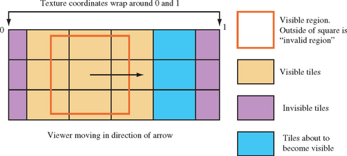
On most systems, texture subimage loads can be very inefficient when narrow regions are being loaded. The subimage loading method can be modified to ensure that only subimage loads above a minimum size are allowed, at the cost of some additional texture memory. The change is simple. Instead of updating every time the view position changes, ignore position changes until the accumulated change requires a subimage load above the minimum size. Normally this will result in some out of date texture data being visible around the edges of the textured geometry. To avoid this, an invalid region is specified around the periphery of the texture level, and the view frustum is adjusted so the that geometry textured from the texels from the invalid region are never visible. This technique allows updates to be cached, improving performance. A wrapped texture with its invalid region is shown in Figure 14.10.
The wrapping technique, as described so far, depends on only a limited region of the textured geometry being visible. In this example we are depending on the limits of the view frustum to only show properly textured geometry. If the view frustum was expanded, we would see the texture image wrapping over the surrounding geometry. Even with these limitations, this technique can be expanded to include mipmapped textures.
Since OpenGL implementations (today) typically do not transparently page mipmaps, the application cannot simply define a very large mipmap and not expect the OpenGL implementation to try to allocate the texture memory needed for all the mipmap levels. Instead the application can use the texture LOD control functionality in OpenGL 1.2 (or the EXT_texture_lod extension) to define a small number of active levels, using the GL_TEXTURE_BASE_LEVEL, GL_TEXTURE_MAX_LEVEL, GL_TEXTURE_MIN_LOD, and GL_TEXTURE_MAX_LOD with the glTexParameter command. An invalid region must be established and a minimum size update must be set so that all levels can be kept in sync with each other when updated. For example, a subimage 32 texels wide at the top level must be accompanied by a subimage 16 texels wide at the next coarser level to maintain correct mipmap filtering. Multiple images at different resolutions will have to be kept in system memory as source images to load texture memory.
If the viewer zooms in or zooms out of the geometry, the texturing system may require levels that are not available in the paged mipmap. The application can avoid this problem by computing the mipmap levels that are needed for any given viewer position, and keeping a set of paged mipmaps available, each representing a different set of LOD levels. The coarsest set could be a normal mipmap for use when the viewer is very far away from that region of textured geometry.
14.6.2 Paging Images in System Memory
Up to this point, we’ve assumed that the texel data is available as a large contiguous image in system memory. Just as texture memory is a limited resource that must be rationed, it also makes sense to conserve system memory. For very large texture images, the image data can be divided into tiles, and paged into system memory from disk. This paging can be kept separate from the paging going on from system memory to texture memory. The only difference will be in the offsets required to index the proper region in system memory to load, and an increase in the number of subimage loads required to update texture memory. A sophisticated system can wrap texture image data in system memory, using modulo arithmetic, just as texture coordinates are wrapped in texture memory.
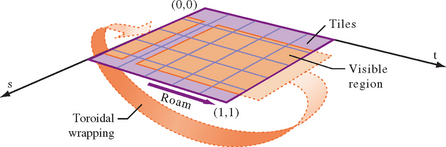
Consider the case of a 2D image roam, illustrated in Figure 14.11, in which the view is moving to the right. As the view pans to the right, new texture tiles must be added to the right edge of the current portion of the texture and old tiles are discarded from the left edge. Since texture wrapping connects these two edges together, the discarding and replacing steps can be combined into a single update step on the tiles that are no longer visible on the left edge, which are about to wrap around and become visible on the right.
The ability to load subregions within a texture has other uses besides these paging applications. Without this capability textures must be loaded in their entirety and their widths and heights must be powers of two. In the case of video data, the images are typically not powers of two, so a texture of the nearest larger power-of-two can be created and only the relevant subregion needs to be loaded. When drawing geometry, the texture coordinates are simply constrained to the fraction of the texture which is occupied with valid data. Mipmapping cannot easily be used with non-power-of-two image data, since the coarser levels will contain image data from the invalid region of the texture. If it’s required, mipmapping can be implemented by padding the non-power-of-two images up to the next power-of-two size, or by using one of the non-power-of-two OpenGL extensions, such as ARB_texture_non_power_of_two, if it is supported by the implementation. Note that not all non-power-of-two extensions support mipmappped non-power-of-two textures.
14.6.3 Hardware Support for Texture Paging
Instead of having to piece together the components of a mipmapped texture paging solution using torroidal mapping, some OpenGL implementations help by providing this functionality in hardware.
Tanner et al. (1998) describe a hardware solution called clip mapping for supporting extremely large textures. The approach is implemented in SGI’s InfiniteReality graphics subsystem. The basic clip mapping functionality is accessed using the SGIX_clipmap extension. In addition to requiring hardware support, the system also requires significant software management of the texture data as well. In part, this is simply due to the massive texture sizes that can be supported. While the clip map approach has no inherent limit to its maximum resolution, the InfiniteReality hardware implementation supports clip map textures to sizes up to 32, 768 × 32, 768 (Montrym et al., 1997).
The clip map itself is essentially a dynamically updatable partial mipmap. Highest resolution texture data is available only around a particular point in the texture called the clip center. To ensure that clip-mapped surfaces are shown at the highest possible texture resolution, software is required to dynamically reposition the clip center as necessary. Repositioning the clip center requires partial dynamic updates of the clip map texture data. With software support for repositioning the clip center and managing the off-disk texture loading and caching required, clip mapping offers the opportunity to dynamically roam over and zoom in and out of huge textured regions. The technique has obvious applications for applications that use very large, detailed textures, such as unconstrained viewing of high-resolution satellite imagery at real-time rates.
Hüttner (1998) describes another approach using only OpenGL’s base mipmap functionality to support very high-resolution textures, similar to the one described previously. Hüttner proposes a data structure called a MIPmap pyramid grid or MP-grid. The MP-grid is essentially a set of mipmap textures arranged in a grid to represent an aggregate high-resolution texture that is larger than the OpenGL implementation’s largest supported texture. For example, a 4×4 grid of 1024×1024 mipmapped textures could be used to represent a 4096×4096 aggregate texture. Typically, the aggregate texture is terrain data intended to be draped over a polygonal mesh representing the terrain’s geometry. Before rendering, the MP-grid algorithm first classifies each terrain polygon based on which grid cells within the MP-grid the polygon covers. During rendering, each grid cell is considered in sequence. Assuming the grid cell is covered by polygons in the scene, the mipmap texture for the grid cell is bound. Then, all the polygons covering the grid cell are rendered with texturing enabled. Because a polygon may not exist completely within a single grid cell, care must be taken to intersect such polygons with the boundary of all the grid cells that the polygon partially covers.
Hüttner compares the MP-grid scheme to the clip map scheme and notes that the MP-grid approach does not require special hardware and does not depend on determining a single viewer-dependent clip center, as needed in the clip map approach. However, the MP-grid approach requires special clipping of the surface terrain mesh to the MP-grid. No such clipping is required when clip mapping. Due to its special hardware support, the clip mapping approach is most likely better suited for the support of the very largest high-resolution textures.
Although not commonly supported at the time of this writing, clip mapping may be an interesting prelude to OpenGL support for dynamically updatable cached textures in future implementations.
14.7 Prefiltered Textures
Currently, some OpenGL implementations still provide limited or no support beyond 4-texel linear isotropic filtering.1 Even when mipmapping, the filtering of each mipmap level is limited to point-sampled (GL_NEAREST) or linear (GL_LINEAR) filtering. While adequate for many uses, there are applications that can greatly benefit from a better filter kernel. One example is anisotropic filtering. Textured geometry can be rendered so that the ideal minification is greater in one direction than another. An example of this is textured geometry that is viewed nearly edge-on. Normal isotropic filtering will apply the maximum required minification uniformly, resulting in excessive blurring of the texture.
If anisotropic texturing is not supported by the implementation,2 the application writer can approach anisotropic sampling by generating and selecting from a series of prefiltered textures. The task of generating and using prefiltered textures is greatly simplified if the application writer can restrict how the texture will be viewed. Prefiltered textures can also be useful for other applications, where the texel footprint isn’t square. If textures are used in such a way that the texel footprints are always the same shape, the number of prefiltered textures needed is reduced, and the approach becomes more attractive.
The technique can be illustrated using anisotropic texturing as an example. Suppose a textured square is rendered as shown in the left of Figure 14.12. The primitive and a selected fragment are shown on the left. The fragment is mapped to a normal mipmapped texture on the upper right, and a prefiltered one on the lower right. In both cases, the ideal texture footprint of the fragment is shown with a dark inner region.
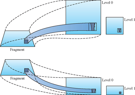
In the upper right texture, the isotropic minification filter forces the actual texture footprint to encompass the square enclosing the dark region. A mipmap level is chosen in which this square footprint is properly filtered for the fragment. In other words, a mipmap level is selected in which the size of this square is closest to the size of the fragment. The resulting mipmap is not level 0 but level 1 or higher. Hence, at that fragment more filtering is needed along t than along s, but the same amount of filtering is done in both. The resulting texture will be more blurred than the ideal.
To avoid this problem, the texture can be prefiltered. In the lower right texture of Figure 14.12, extra filtering is applied in the t direction when the texture is created. The aspect ratio of the texture image is also changed, giving the prefiltered texture the same width but only half the height of the original. The footprint now has a squarer aspect ratio; the enclosing square no longer has to be much larger, and is closer to the size to the fragment. Mipmap level 0 can now be used instead of a higher level. Another way to think about this concept: using a texture that is shorter along t reduces the amount of minification required in the t direction.
The closer the filtered mipmap’s aspect ratio matches the projected aspect ratio of the geometry, the more accurate the sampling will be. The application can minimize excessive blurring at the expense of texture memory by creating a set of resampled mipmaps with different aspect ratios (Figure 14.13).
14.7.1 Computing Texel Aspect Ratios
Once the application has created a set of prefiltered textures, it can find the one that most closely corresponds to the current texture scaling aspect ratio, and use that texture map to texture the geometry (Figure 14.14). This ratio can be quickly estimated by computing the angle between the viewer’s line of sight and a plane representing the orientation of the textured geometry. Using texture objects, the application can switch to the mipmap that will provide the best results. Depending on performance requirements, the texture selection process can be applied per triangle or applied to a plane representing the average of a group of polygons can be used.
In some cases, a simple line of sight computation isn’t accurate enough for the application. If the textured surface has a complex shape, or if the texture transform matrix is needed to transform texture coordinates, a more accurate computation of the texture coordinate derivatives may be needed. Section 13.7.2 describes the process of computing texture coordinate derivatives within the application. In the near future the programmable pipeline will be capable of performing the same computations efficiently in the pipeline and be able to select from one of multiple-bound texture maps.
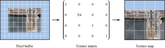
Since most OpenGL implementations restrict texture levels to have power-of-two dimensions, it would appear that the only aspect ratios that can be anisotropically pre-filtered are 1:4, 1:2, 1:1, 2:1, 4:1, etc. Smaller aspect ratio step sizes are possible, however, by generating incomplete texture images, then using the texture transform matrix to scale the texture coordinates to fit. For a ratio of 3:4, for example, fill a 1:1 ratio mipmap with prefiltered 3:4 texture images partially covering each level (the rest of the texture image is set to black). The unused part of the texture (black) should be along the top (maximum t coordinates) and right (maximum s coordinates) of the texture image. The prefiltered image can be any size, as long as it fits within the texture level. Other than prefiltering the images, the mipmap is created in the normal way.
Using this mipmap for textured geometry with a 3:4 ratio results in an incorrect textured image. To correct it, the texture transform matrix is used to rescale the narrower side of the texture (in our example in the t direction) by 3/4 (Figure 14.15). This will change the apparent size ratio between the pixels and textures in the texture filtering system, making them match, and producing the proper results. This technique would not work well with a repeated texture; in our example, there will be a discontinuity in the image if filtered outside the range of 0 to 1 in t. However, the direction that isn’t scaled can be wrapped; in our example, wrapping in s would work fine.
Generalizing from the previous example, the prefiltering procedure can be broken down as follows:
1. Look for textures that have elongated or distorted pixel footprints.
2. Determine the range of pixel footprint shapes on the texture of interest to determine the number of prefiltered images needed.
3. Using convolution or some other image processing technique (see Chapter 12), prefilter the image using the footprint shape as a filter kernel. The prefiltered images should be filtered from higher resolution images to preserve image quality.
4. Generate a range of prefiltered textures matching the range of footprint shapes.
5. Design an algorithm to choose the most appropriate prefiltered image for the texture’s viewing conditions.
6. The texture transform matrix can be used to change the relationship between texture and geometric coordinates to support a wider range of prefiltered images.
Prefiltered textures are a useful tool but have limitations compared to true anisotropic texturing. Storing multiple prefiltered images consumes a lot of texture memory; the algorithm is most useful in applications that only need a small set of prefiltered images to choose from. The algorithm for choosing a prefiltered texture should be simple to compute; it can be a performance burden otherwise, since it may have to be run each time a particular texture is used in the scene. Prefiltered images are inadequate if the pixel footprint changes significantly while rendering a single texture; segmenting the textured primitive into regions of homogeneous anisotropy is one possible solution, although this can add still more overhead. Dynamically created textures are a difficult obstacle. Unless they can be cached and reused, the application may not tolerate the overhead required to prefilter them on the fly.
On the other hand, the prefiltered texture solution can be a good fit for some applications. In visual simulation applications, containing fly-over or drive-through viewpoints, prefiltering the terrain can lead to significant improvements in quality without high overhead. The terrain can be stored prefiltered for a number of orientations, and the algorithm for choosing the anisotropy is a straightforward analysis of the viewer/terrain orientation. The situation is further simplified if the viewer has motion constraints (for example, a train simulation), which reduce the number of prefiltered textures needed.
Hardware anisotropic filtering support is a trade-off between filtering quality and performance. Very high-quality prefiltered images can be produced if the pixel footprint is precisely known. A higher-quality image than what is achievable in hardware can also be created, making it possible to produce a software method for high-quality texturing that discards all the speed advantages of hardware rendering. This approach might be useful for non-real-time, high-quality image generation.
14.8 Dual-Paraboloid Environment Mapping
An environment map parameterization different from the ones directly supported by OpenGL (see Section 5.4) was proposed by Heidrich and Seidel (1998b). It avoids many of the disadvantages of sphere mapping. The dual-paraboloid environment mapping approach is view-independent, has better sampling characteristics, and, because the singularity at the edge of the sphere map is eliminated, there are no sparkling artifacts at glancing angles. The view-independent advantage is important because it allows the viewer, environment-mapped object, and the environment to move with respect to each other without having to regenerate the environment map.
14.8.1 The Mathematics of Dual-Paraboloid Maps
The principle that underlies paraboloid maps is the same one that underlies a parabolic lens or satellite dish. The geometry of a paraboloid can focus parallel rays to a point.
The paraboloid used for dual-paraboloid mapping is:
Figure 14.16 shows how two paraboloids can focus the entire environment surrounding a point into two images.
Unlike the sphere-mapping approach, which encodes the entire surrounding environment into a single texture, the dual-paraboloid mapping scheme requires two textures to store the environment, one texture for the “front” environment and another texture for the “back”. Note that the sense of “front” and “back” is completely independent of the viewer orientation. Figure 14.17 shows an example of two paraboloid maps. Because two textures are required, the technique must be performed in two rendering passes.
If multitexturing is supported by the implementation, the passes can be combined into a single rendering pass using two texture units.
Because the math for the paraboloid is all linear (unlike the spherical basis of the sphere map), Heidrich and Seidel observe that an application can use the OpenGL texture matrix to map an eye-coordinate reflection vector R into a 2D texture coordinate (s, t) within a dual-paraboloid map. The necessary texture matrix can be constructed as follows:
where
is a matrix that scales and biases a 2D coordinate in the range [−1, 1] to the texture image range [0, 1]. This matrix
is a projective transform that divides by the z coordinate. It serves to flatten a 3D vector into 2D. This matrix
subtracts the supplied 3D vector from an orientation vector D that specifies a view direction. The vector is set to D either (0, 0, − 1)T or (0, 0, 1)T depending on whether the front or back paraboloid map is in use, respectively. Finally, the matrix (Ml)−1 is the inverse of the linear part (the upper 3×3) of the current (affine) modelview matrix. The matrix (Ml)−1 transforms a 3D eye-space reflection vector into an object-space version of the vector.
14.8.2 Using Dual-Paraboloid Maps
For the rationale for these transformations, consult Heidrich and Siedel (1998b). Since all the necessary component transformations can be represented as 4×4 matrices, the entire transformation sequence can be concatenated into a single 4×4 projective matrix and then loaded into OpenGL’s texture matrix. The per-vertex eye-space reflection normal can be supplied as a vertex texture coordinate via glTexCoord3f or computed from the normal vector using the GL_REFLECTION_MAP texture coordinate generation mode.3 When properly configured this 3D vector will be transformed into a 2D texture coordinate in a front or back paraboloid map, depending on how D is oriented.
The matrix Ml−1 is computed by retrieving the current modelview matrix, replacing the outer row and column with the vector (0, 0, 0, 1), and inverting the result. Section 13.1 discusses methods for computing the inverse of the modelview matrix.
Each dual-paraboloid texture contains an incomplete version of the environment. The two texture maps overlap as shown in Figure 14.17 at the corner of each image. The corner regions in one map are distorted so that the other map has better sampling of the same information. There is also some information in each map that is simply not in the other; for example, the information in the center of each map is not shared. Figure 14.18 shows that each map has a centered circular region containing texels with better sampling than the corresponding texels in the other map. This centered region of each dual-paraboloid map is called the sweet circle.
The last step is to segregate transformed texture coordinates, applying them to one of the two paraboloid maps. The decision criteria are simple; given the projective transformation discussed earlier, if a reflection vector falls within the sweet circle of one dual-paraboloid map, it will be guaranteed to fall outside the sweet circle of the opposite map.
Using OpenGL’s alpha testing capability, we can discard texels outside the sweet circle of each texture. The idea is to encode in the alpha channel of each dual-paraboloid texture an alpha value of 1.0 if the texel is within the sweet circle and 0.0 if the texel is outside the sweet circle. To avoid artifacts for texels that land on the circle edges, the circle ownership test should be made conservative.
In the absence of multitexture support, a textured object is rendered in two passes. First, the front dual-paraboloid texture is bound and the D value is set to (0, 0,−1)T when constructing the texture matrix. During the second pass, the back texture is bound and a D value of (0, 0, 1)T is used. During both passes, alpha testing is used to eliminate fragments with an alpha value less than 1.0. The texture environment should be configured to replace the fragment’s alpha value with the texture’s alpha value. The result is a complete dual-paraboloid mapped object.
When multiple texture units are available, the two passes can be collapsed into a single multitextured rendering pass. Since each texture unit has an independent texture matrix, the first texture unit uses the front texture matrix, while the second texture unit uses the back one. The first texture unit uses a GL_REPLACE texture environment while the second texture unit should use GL_BLEND. Together, the two texture units blend the two textures based on the alpha component of the second texture. A side benefit of the multitextured approach is that the transition between the two dual-paraboloid map textures is less noticeable. Even with simple alpha testing, the seam is quite difficult to notice.
If a programmable vertex pipeline is supported, the projection operation can be further optimized by implementing it directly in a vertex program.
14.8.3 OpenGL Dual-Paraboloid Support
Although OpenGL doesn’t include direct support for dual-paraboloid maps, OpenGL 1.3 support for reflection mapping and multitexture allows efficient implementation by an application. The view independence, good sampling characteristics, and ease of generation of maps makes dual-paraboloid maps attractive for many environment mapping applications.
Besides serving as an interesting example of how OpenGL functionality can be used to build up an entirely new texturing technique, dual-paraboloid mapping is also a useful approach to consider when the OpenGL implementation doesn’t support cube mapping. This technique provides some clear advantages over sphere mapping; when the latter isn’t adequate, and the rendering resources are available, dual-paraboloid mapping can be a good high-performance solution.
14.9 Texture Projection
Projected textures (Segal et al., 1992) are texture maps indexed by texture coordinates that have undergone a projective transform. The projection is applied using the texture transform matrix, making it possible to apply a projection to texture coordinates that is independent of the geometry’s viewing projection. This technique can be used to simulate slide projector or spotlight illumination effects, to apply shadow textures (Section 17.4.3), create lighting effects (Section 15.3), and to re-project an image onto an object’s geometry (Section 17.4.1).
Projecting a texture image onto geometry uses nearly the same steps needed to project the rendered scene onto the display. Vertex coordinates have three transformation stages available for the task, while texture coordinates have only a single 4×4 transformation matrix followed by a perspective divide operation. To project a texture, the texture transform matrix contains the concatenation of three transformations:
1. A modelview transform to orient the projection in the scene.
2. A projective transform (e.g., perspective or parallel).
3. A scale and bias to map the near clipping plane to texture coordinates, or put another way, to map the [−1, 1] normalized device coordinate range to [0, 1].
When choosing the transforms for the texture matrix, use the same transforms used to render the scene’s geometry, but anchored to the view of a “texture light", the point that appears to project the texture onto an object, just as a light would project a slide onto a surface. A texgen function must also be set up. It creates texture coordinates from the vertices of the target geometry. Section 13.6 provides more detail and insight in setting up the proper texture transform matrix and texgen for a given object/texture configuration.
Configuring the texture transformation matrix and texgen function is not enough. The texture will be projected onto all objects rendered with this configuration; in order to produce an “optical” projection, the projected texture must be “clipped” to a single area.
There are a number of ways to do this. The simplest is to only render polygons that should have the texture projected on them. This method is fast, but limited; it only clips the projected texture to the boundaries defined by individual polygons. It may be necessary to limit the projected image within a polygon. Finer control can be achieved by using the stencil buffer to control which parts of the scene are updated by a projected texture. See Section 14.6 for details.
If the texture is non-repeating and is projected onto an untextured surface, clipping can be done by using the GL_MODULATE environment function with a GL_CLAMP texture wrap mode and a white texture border color. As the texture is projected, the surfaces beyond the projected [0, 1] extent are clamped and use the texture border color. They end up being modulated with white, leaving the areas textured with the border color unchanged. One possible problem with this technique is poor support of texture borders on some OpenGL implementations. This should be less of a problem since the borders are a constant color. There are other wrap modes, such as GL_CLAMP_TO_BORDER, which can be used to limit edge sampling to the border color.
The parameters that control filtering for projective textures are the same ones controlling normal texturing; the size of the projected texels relative to screen pixels determines minification or magnification. If the projected image is relatively small, mipmapping may be required to get good quality results. Using good filtering is especially important if the projected texture is being applied to animated geometry, because poor sampling can lead to scintillation of the texture as the geometry moves.
Projecting a texture raises the issue of perspective correct projection. When texture coordinates are interpolated across geometry, use of the transformed w coordinate is needed to avoid artifacts as the texture coordinates are interpolated across the primitive, especially when the primitive vertices are projected in extreme perspective. When the texture coordinates themselves are projected, the same “perspective correct” issue (see Section 6.1.4) must be dealt with (Figure 14.19).
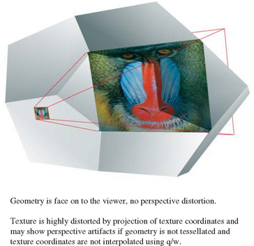
The problem is avoided by interpolating the transformed q coordinate, along with the other texture coordinates. This assures that the texture coordinates are interpolated correctly, even if the texture image itself is projected in extreme perspective. For more details on texture coordinate interpolation see Section 5.2. Although the specification requires it, there may be OpenGL implementations that do not correctly support this interpolation. If an implementation doesn’t interpolate correctly, the geometry can be more finely tessellated to minimize the difference in projected q values between vertices.
Like viewing projections, a texture projection only approximates an optical projection. The geometry affected by a projected texture won’t be limited to a region of space. Since there is no implicit texture-space volume clipping (as there is in the OpenGL viewing pipeline), the application needs to explicitly choose which primitives to render when a projected texture is enabled. User-defined clipping planes, or stencil masking may be required if the finer control over the textured region is needed.
14.10 Texture Color Coding and Contouring
Texture coordinate generation allows an application to map a vertex position or vector to a texture coordinate. For linear transforms, the transformation is texcoord = f(x, y, z, w), where texcoord can be any one of s, t, r, or q, and f(x, y, z, w) = Ax + By + Cz + Dw, where the coefficients are set by the application. The generation can be set to happen before or after the modelview transform has been applied to the vertex coordinates. See Section 5.2.1 for more details on texture coordinate generation.
One interesting texgen application is to use generated texture coordinates as measurement units. A texture with a pattern or color coding can be used to delimit changes in texture coordinate values. A special texture can be applied to target geometry, marking the texture coordinate changes across its surface visible. This approach makes it possible to annotate target geometry with measurement information. If relationships between objects or characteristics of the entire scene need to be measured, the application can create and texture special geometry, either solid or semitransparent, to make these values visible.
One or more texture coordinates can be used simultaneously for measurement. For example, a terrain model can be colored by altitude using a 1D texture map to hold the coloring scheme. The texture can map s as the distance from the plane y = 0, for example. Generated s and t coordinates can be mapped to the x = 0 and z = 0 planes, and applied to a 2D texture containing tick marks, measuring across a 2D surface.
Much of the flexibility of this technique comes from choosing the appropriate measuring texture. In the elevation example, a 1D texture can be specified to provide different colors for different elevations, such as that used in a topographic map. For example, if vertex coordinates are specified in meters, distances less than 50 meters can be colored blue, from 50 to 800 meters in green, and 800 to 1000 meters in white. To produce this effect, a 1D texture map with the first 5% blue, the next 75% green, and the remaining 20% of texels colored white is needed. A 64- or 128-element texture map provides enough resolution to distinguish between levels. Specifying GL_OBJECT_LINEAR for the texture generation mode and an GL_OBJECT_PLANE equation of (0, 1/1000, 0, 0) for the s coordinate will set s to the y value of the vertex scaled by 1/1000 (i.e., s = (0,1/1000,0, 0)· (x, y, z, w)).
Different measuring textures provide different effects. Elevation can be shown as contour lines instead of color coding, using a 1D texture map containing a background color, marked with regularly spaced tick marks. Using a GL_REPEAT wrap mode creates regularly repeating lines across the object being contoured. Choosing whether texture coordinate generation occurs before or after the modelview transform affects how the measuring textures appear to be anchored. In the contour line example, a GL_OBJECT_LINEAR generation function anchors the contours to the model (Figure 14.20). A GL_EYE_LINEAR setting generates the coordinates in eye space, fixing the contours in space relative to the viewer.
Textures can do more than measure the relative positions of points in 3D space; they can also measure orientation. A sphere or cube map generation function with an appropriately colored texture map can display the orientation of surface normals over a surface. This functionality displays the geometry’s surface orientation as color values on a per-pixel basis. Texture sampling issues must be considered, as they are for any texturing application. In this example, the geometry should be tessellated finely enough that the change in normal direction between adjacent vertices are limited enough to produce accurate results; the texture itself can only linearly interpolate between vertices.
14.11 2D Image Warping
OpenGL can warp an image by applying it to a surface with texturing. The image is texture mapped onto planar geometry, using non-uniform texture coordinates to distort it. Image warping takes advantage of OpenGL’s ability to establish an arbitrary relationship between texture coordinates and vertex coordinates. Although any geometry can be used, a common technique is to texture onto a uniform polygonal mesh, adjusting the texture coordinates at each vertex on the mesh. This method is popular because the mesh becomes a regular sampling grid, and the changes in texture coordinates can be represented as a function of the texture coordinate values. The interpolation of texture coordinates between vertices gives the warp a smooth appearance, making it possible to approximate a continuous warping function.
Warping may be used to change the framebuffer image (for example, to create a fish-eye lens effect), or as part of preprocessing of images used in texture maps or bitmaps. Repeated warping and blending steps can be concatenated to create special effects, such as streamline images used in scientific visualization (see Section 20.6.3). Warping can also be used to remove distortion from an image, undoing a preexisting distortion, such as that created by a camera lens (see Section 12.7.4).
A uniform mesh can be created by tessellating a 2D rectangle into a grid of vertices. In the unwarped form, texture coordinates ranging from zero to one are distributed evenly across the mesh. The number of vertices spanning the mesh determines the sampling rate across the surface. Warped texture coordinates are created by applying the 2D warping function warp(s, t) = (s + Δs, t + Δt) to the unwarped texture coordinates at each vertex in the mesh. The density of vertices on the mesh can be adjusted to match the amount of distortion applied by the warping function; ideally, the mesh should be fine enough that the change in the warped coordinate is nearly linear from point to point (Figure 14.21). A sophisticated scheme might use non-linear tessellation of the surface to ensure good sampling. This is useful if the warping function produces a mixture of rapidly changing and slowly changing warp areas.
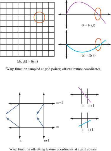
The warped texture coordinates may be computed by the application when the mesh is created. However, if the warp can be expressed as an affine or projective transform, a faster method is to modify the texture coordinates with the texture transform matrix.
This takes advantage of the OpenGL implementation’s acceleration of texture coordinate transforms. An additional shortcut is possible; texgen can be configured to generate the unwarped texture coordinate values. How the image is used depends on the intended application.
By rendering images as textured geometry, warped images are created in the framebuffer (usually the back buffer). The resultant image can be used as-is in a scene, copied into a texture using glCopyTexImage2D, or captured as an application memory image using glReadPixels.
The accuracy of the warp is a function of the texture resolution, the resolution of the mesh (ratio of the number of vertices to the projected screen area), and the filtering function used with the texture. The filtering is generally GL_LINEAR, since it is a commonly accelerated texture filtering mode, although mipmapping can be used if the distortion creates regions where many texels are to be averaged into a single pixel color.
The size of the rendered image is application-dependent; if the results are to be used as a texture or bitmap, then creating an image larger than the target size is wasteful; conversely, too small an image leads to coarse sampling and pixel artifacts.
14.12 Texture Animation
Although movement and change in computer graphics is commonly done by modifying geometry, animated surface textures are also a useful tool for creating dynamic scenes. Animated textures make it possible to add dynamic complexity without additional geometry. They also provide a flexible method for integrating video and other dynamic image-based effects into a scene. Combining animated images and geometry can produce extremely realistic effects with only moderate performance requirements. Given a system with sufficient texture load and display performance, animating texture maps is a straightforward process.
Texture animation involves continuously updating the image used to texture a surface. If the updates occur rapidly enough and at regular intervals, an animated image is generated on the textured surface. The animation used for the textures may come from a live external source, such as a video capture device, a pre-recorded video sequence, or pre-rendered images.
There are two basic animation approaches. The first periodically replaces the contents of the texture map by loading new texels. This is done using the glTexSubImage2D command. The source frames are transfered from an external source (typically disk or video input) to system memory, then loaded in sequence into texture memory. If the source frames reside on disk, groups of source frames may be read into memory. The memory acts as a cache, averaging out the high latency of disk transfers, making it possible to maintain the animation update rate.
The second animation approach is useful if the number of animated images is small (such as a small movie loop). A texture map containing multiple images is created; the texture is animated by regularly switching the image displayed. A particular image is selected by changing the texture coordinates used to map the texture onto the image. This can be done explicitly when sending the geometry, or by using texgen or the texture transform matrix.
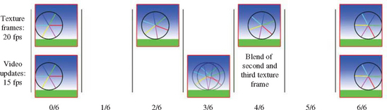
When discussing animation update rates, there are two parameters to consider: the rate at which an animated texture is updated, and the frame rate at which the graphics application updates the scene. The two are not necessarily the same. The animation frame rate may be higher or lower than the scene frame rate. Ideally, the updates to the texture map should occur at the scene frame rate. If the source animation was recorded at a different rate, it needs to be resampled to match the scene’s rate.
If the animation rate is an even multiple of each other, then the resampling algorithm is trivial. If for example, the animation rate is one half of the frame rate, then resampling means using each source animation image twice per frame. If the animation rates do not have a 1/n relationship, then the texture animation may not appear to have a constant speed.
To improve the update ratios, the animation sequence can be resampled by linearly interpolating between adjacent source frames (Figure 14.22). The resampling may be performed as a preprocessing step or be computed dynamically while rendering the scene. If the resampling is performed dynamically, texture environment or framebuffer blending can be used to accelerate the interpolation.
Note that resampling must be done judiciously to avoid reducing the quality of the animation. Interpolating between two images to create a new one does not produce the same image that would result from sampling an image at that moment in time. Interpolation works best when the original animation sequence has only small changes between images. Trying to resample an animation of rapidly changing, high-contrast objects with interpolation can lead to objects with “blurry” or “vibrating” edges.
Choosing the optimal animation method depends on the number of frames in the animation sequence. If the number of frames is unbounded, such as animation from a streaming video source, continuously loading new frames will be necessary. However, there is a class of texture animations that use a modest, fixed number of frames. They are played either as an endless loop or as a one-shot sequence. An example of the first is a movie loop of a fire applied to a texture for use in a torch. An example one-shot sequence is a short animation of an explosion. If the combined size of the frames is small enough, the entire sequence can be captured in a single texture.
Even when space requirements prohibit storing the entire image sequence, it can still be useful to store a group of images at a time in a single texture. Batching images this way can improve texture load efficiency and can facilitate resampling of frames before they are displayed.
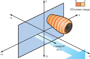
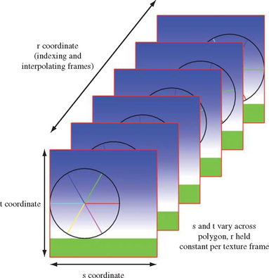
There are two obvious approaches to storing multiple frames in a single texture map. A direct method is to use a 3D texture map. The 3D texture is created from a stack of consecutive animation frames. The s and t coordinates index the horizontal and vertical axis of each image; the r coordinate represents the time dimension. Creating a 3D texture from stack of images is simple; load the sequence of images into consecutive locations in memory, then use glTexImage3D to create the 3D texture map from the data. OpenGL implementations limit the maximum dimensions and may restrict other 3D texture parameters, so the usual caveats apply.
Rendering from the 3D texture is also simple. The texture is mapped to the target geometry using s and t coordinates as if it’s a 2D texture. The r coordinate is set to a fixed value for all vertices in the geometry representing the image. The r value specifies a moment in time in the animation sequence (Figure 14.23). Before the next frame is displayed, r is incremented by an amount representing the desired time step between successive frames. 3D textures have an inherent benefit; the time value doesn’t have to align with a specific image in the texture. If GL_LINEAR filtering is used, an r value that doesn’t map to an exact animation frame will be interpolated from the two frames bracketing that value, resampling it. Resampling must be handled properly when a frame must sample beyond the last texture frame in the texture or before the first. This can happen when displaying an animation loop. Setting the GL_TEXTURE_WRAP_R parameter to GL_REPEAT ensures that the frames are always interpolating valid image data.
Although animating with 3D textures is conceptually simple, there are some significant limitations to this approach. Some implementations don’t support 3D texture mapping (it was introduced in OpenGL 1.2), or support it poorly, supporting only very small 3D texture maps. Even when they are supported, 3D textures use up a lot of space in texture memory, which can limit their maximum size. If more frames are needed than fit in a 3D texture, another animation method must be used, or the images in the 3D texture must be updated dynamically. Dynamic updates involve using the glTexSubImage command to replace one or more animation frames as needed. In some implementations, overall bandwidth may improve if subimage loads take place every few frames and load more than one animation frame at a time. However, the application must ensure that all frames needed for resampling are loaded before they are sampled.
A feature of 3D texture mapping that can cause problems is mipmap filtering. If the animated texture requires mipmap filtering (such as an animated texture display on a surface that is nearly edge on to the viewer), a 3D texture map can’t be used. A 3D texture mipmap level is filtered in all three dimensions (isotropically). This means that a mipmapped 3D texture uses much more memory than a 2D mipmap, and that LODs contain data sampled in three dimensions. As a result, 3D texture LOD levels resample frames, since they will use texels along the r-axis.
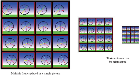
Another method for storing multiple animation frames is to mosaic the frames into a single 2D texture. The texture map is tiled into a mosaic of images, each frame is loaded into a specific region. To avoid filtering artifacts at the edges of adjacent images, some basic spacing restrictions must be obeyed (see Section 14.4 for information on image mosaicing). The texture is animated by adjusting the texture coordinates of the geometry displaying the animation so that it references a different image each frame. If the texture has its animation frames arranged in a regular grid, it becomes simple to select them using the texture matrix. There are a number of advantages to the mosaic approach: individual animation frames do not need to be padded to be a power-of-two, and individual frames can be mipmapped (assuming the images are properly spaced (Figure 14.24). The fact than any OpenGL implementation can support mosaicing, and that most implementations can support large 2D textures, are additional advantages.
Texture mosaicing has some downsides. Since there is no explicit time dimension, texturing the proper frame requires more texture coordinate computation than the 3D texture approach does. Texture mosaicing also doesn’t have direct support for dynamic frame resampling, requiring more work from the application. It must index the two closest images that border the desired frame time, then perform a weighted blend of them to create the resampled one, using weighting factors derived from the resampled frame’s relationship with the two parent images. The blending itself can be done using a multitexture or a multipass blend technique (see Section 5.4 and Section 6.2.4 for details on these approaches).
Even when using 2D textures, the amount of space required for the animation frames may exceed the capacity of the texture map. In this case, dynamic updates of the images in the texture are necessary. When incremental updates are required, and the animation uses frame resampling, care should be taken to ensure that all images required for resampling are completely loaded before they are displayed. In general, one texture (or two if frames are being resampled) is in use at any time during animation. If dynamic updates are required, it is important to only replace images that aren’t being used for texturing. To do this, a double buffering or multibuffering approach can be implemented. The images in the texture are grouped into two or more blocks, and only blocks not being used for texturing are candidates for updating. Again, care must be taken to ensure that an inactive block of images won’t be accessed before the load completes. In some cases, it can help to duplicate images at the borders of the blocks to ease load requirements at the cost of some additional texture memory.
14.13 Detail Textures
Textures, even mipmapped ones, appear unrealistic under strong magnification. When the viewer is close to a texture surface, a single texel color is filtered over multiple pixels. Under this strong magnification, linear filtering results in an unrealistically smoothed image with little surface detail. Not only do the magnified images look unrealistic, but the lack of high-frequency spatial information on the surface makes it difficult for a viewer to get realistic distance and motion cues when moving near the surface.
Ideally, a mipmapped texture will have enough high-resolution levels that any normal view of the textured surface will always have sufficient high-frequency spatial data. But providing extra high-resolution levels is expensive; they take up a disproportionate amount of texture memory. With mipmapping, each fine level requires four times as many texels as the next coarser one. In addition to the texture memory overhead, obtaining the high-resolution data can be expensive. For some applications, it is worth the effort. Finer levels may contain valuable visual details; they can provide useful information or add realism to the surface.
In many cases, however, the close-up details are not significant. A very high-resolution surface image will contain details, but these details may be of little value. An example may be a close-up view of an asphalt highway; the imperfections revealed may be of little interest to the viewer. Detail at this level can also be very self-similar; in our roadside example, one section of asphalt detail may look very similar to any other. Although the details may not be visually interesting, some fine level detail can provide important visual cues about the viewer’s distance and velocity relative to the surface, and keep the surface from looking blurry.
A detail texture can be a useful approach in these circumstances (Figure 14.25). Instead of making more high-resolution levels, a texture is created that contains only high-frequency details from the surface. The detail texture is not an entire high-resolution level, however. Instead a smaller image is used, and replicated across the surface to cover it. This approach takes advantage of some features of high-frequency details; the details are often self-similar, so a small patch can be replicated across the surface without looking too uniform. Since the detail texture contains only high-frequency image features, they change rapidly across the texture. There are no low-frequency components that would generate tiling artifacts when the texture is repeated.
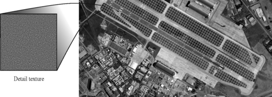
The pairing of a base mipmap with the appropriate detail texture is a powerful combination. The mipmapped texture contains levels that provide a realistic representation of the surface, but does not contain the highest frequency detail. The detail texture provides fine, high-frequency features, which are only needed when the viewer is close to the textured surface. When the viewer gets close enough, both textures are applied; the detail texture is scaled up to become more prominent as the viewer approaches.
The extra work in implementing detail textures comes from the controlled application of base and detail texture images. Detail textures should not contribute anything when the base texture is not magnifying. The high-frequency component intensity should be a function of the base texture’s magnification level.
The relative texture intensities can be implemented by blending, either by alpha blending fragments, or by using multitexturing. The relative intensities should be a function of base texture magnification. A less computationally expensive approach is is to estimate the magnification level by computing it as a function of viewer distance. Constraints specific to the application can simplify the problem in some cases. A flight simulator, for example, may use the height above ground and a precomputed scaling factor to estimate the texture magnification level of the terrain (Figure 14.26). If the simulator’s view frustum brings the entire visible textured surface into view at nearly the same magnification, this approximation will be sufficiently accurate to provide a realistic effect.
In the general case, however, computing texture magnification can be difficult. An accurate computation of texture magnification must consider the visible vertices of the textured surface, the texture coordinate scaling resulting from the current modelview and projection transformations, the current texture coordinate generation settings, and the values of the texture transformation matrix. Section 13.7.2 discusses the steps in the computation in more detail. The best place to perform these computations is in the OpenGL implementation; to some extent this can be achieved in the programmable pipeline within a fragment program. There is also a vendor-specific detail texture extension SGIS_detail_texture. This extension blends in the detail texture as a function of magnification, and allows the detail texture either to add to or modulate the base texture. Unfortunately, it’s unlikely to see widespread adoption, but the ideas present in it are or will be supportable using fragment programs.
14.13.1 Signed Intensity Detail Textures
Signed detail textures can be applied accurately without necessarily using separate texture magnification computations. A detail texture image is created that contains signed intensity values. The values are chosen so that the average value of the texel elements are zero. When combined with the base texture, the detail texture modifies its color values, adding high-frequency components to the textured image. Since the detail texture values average to zero intensity, a minified detail texture doesn’t contribute to the overall image. This feature makes the fade in of texture detail “automatic", so no special computations are needed to selectively blend in detail.
The detail texture is applied to the same geometry as the base texture. The texture coordinates applied to both textures are adjusted so that the detail texture minifies if the base texture is not magnifying. The minification filtering will cause the signed intensity components to blend together. One way of making the detail texture “average out” is to make a mipmap out of it. The coarser mipmap levels of the detail texture will average more of its components, causing it to gradually fade out. As both the detail and base texture are zoomed, the detail texture will filter to its finer LOD levels, and the signed intensity values stop canceling each other out.
The fixed-function OpenGL pipeline doesn’t support signed texture color components, but only values ranging from [0, 1]. To implement signed arithmetic, the implementation must use a representation of signed numbers that are biased (and possibly scaled) to remain in the [0, 1] range (Section 3.4.1). The detail texture is added to the base texture using either multiple texture units or multiple passes and framebuffer blending.
In the multipass solution, the surface is first rendered with the base texture. The texture is applied as normal; configured to modulate the polygon color to capture vertex lighting detail, for example. The second step applies the detail texture. Since the detail texture is smaller than the base texture, and is generally applied using GL_REPEAT wrapping, the texture coordinates used differ from those used with the base texture. This change in mapping can be accomplished by using a separate set of per-vertex texture coordinates, generating coordinates using texgen, or by modifying the texture transformation matrix.
Neither the texture environment nor alpha blend stages support signed values; in both cases, the color and alpha component values are expected to range from [0, 1]. Despite this limitation, both stages can be configured to handle signed quantities, by representing the signed numbers in a biased format. Besides offering only a limited range, OpenGL only supports a limited (implementation-dependent) precision for the color component values. Care must be taken not to overly reduce this precision while processing colors. For whatever color format is chosen, the algebra for combining textures must follow certain rules in order to produce the desired results. When the base texture color is modified by a signed detail texture color, a detail color of zero should not change the base color, while a positive or negative detail color should increase or decrease the intensity of the base color, respectively. If the resulting base color goes out of its [0, 1] range, it will be clamped.
Since the detail texture’s values are meant to modify the base color, there is some flexibility in specifying its range. The ideal range is [−1, 1], since that allows a detail texture color component to drive the base color component over the entire range of values, regardless of the base texture’s color. Mathematically, the detail texture’s [0, 1] range is scaled by 2 and biased by − 1 to put its values in the range [−1, 1]. This value is then added to the unmodified base texture, and the results are clamped to [0, 1]. These operations can be condensed to the equation:
Note that this approach assumes that intermediate results are not clamped to [0, 1], which is not generally true in all OpenGL implementations.
For many applications, the detail texture does not need to be able to drive the base texture to an arbitrary value, since the goal of the detail texture is to only pattern the base texture with detail, not replace it. In many cases, a more limited range of ![]() is sufficient. This range is particularly useful, since it can be derived from the normal [0, 1] texture representation without scaling. The detail needs only to be biased by
is sufficient. This range is particularly useful, since it can be derived from the normal [0, 1] texture representation without scaling. The detail needs only to be biased by ![]() . Mathematically, the two textures are combined with:
. Mathematically, the two textures are combined with:
As before, this approach runs into problems if intermediate results are clamped to [0, 1]. However, the GL_COMBINE texture environment function supports the ![]() range detail texture representation directly, with the GL_ADD_SIGNED texture function. It implements the equation Arg0+Arg1−0.5, and doesn’t clamp the intermediate results. This allows the signed detail sum to be implemented in a single pass using two texture units. The first unit applies the base texture to the geometry, the second adds the detail texture using the GL_ADD_SIGNED operation.
range detail texture representation directly, with the GL_ADD_SIGNED texture function. It implements the equation Arg0+Arg1−0.5, and doesn’t clamp the intermediate results. This allows the signed detail sum to be implemented in a single pass using two texture units. The first unit applies the base texture to the geometry, the second adds the detail texture using the GL_ADD_SIGNED operation.
Modulating Detail
A useful variation of the signed detail texture approach is to modulate rather than add the detail texture component to the base texture. This amplifies variation by scaling rather than adding and subtracting variation. Signed values aren’t very useful for the modulation case; instead, the detail texture values are greater than or less than one. A simple implementation uses a range of [0, 2], which can be derived from OpenGL texture values in the range [0, 1] with a scale value of two. This range of values makes it possible to force the base texture to a reasonable range of values. Note that detail texture values of ![]() are scaled to one, which will not modify the base texture. The detail texture should average out to this value, in order to fade out under minification.
are scaled to one, which will not modify the base texture. The detail texture should average out to this value, in order to fade out under minification.
As with additive detail textures, a modulating detail texture can be implemented with texture environment functionality partnered with multitexturing. The multitexturing case is straightforward. Unit 0 applies the base texture to the surface, unit 1 modulates the base by the detail texture, then scales the result by two using GL_RGB_SCALE. The results are implicitly clamped to the range [0, 1] after scaling.
Implementing this algorithm using framebuffer blending is awkward but possible. The base textured geometry, once rendered to the framebuffer, can be modulated by the detail texture using a blending function of GL_ZERO, GL_SRC_COLOR. Since there is no support for a scale factor greater than one, the results of combining the base and detail textures must be added to the framebuffer twice. This can be done by reading back the framebuffer, then blending it in again, using a blend function of GL_ONE, GL_ONE.
Modulating detail textures are very useful when the base texture modulates vertex-lighted geometry. Modulating ensures that the detail texture changes follow the shading imposed by the lighting model, just as the base texture does. Additive detail textures do not take base texture value changes into account and will appear unlighted.
14.13.2 Creating Detail Textures
While a detail texture can contain a high-frequency pattern that is independent of the base texture, the best results are obtained when it contains the high-frequency components derived from the original image. The first step toward extracting detail texture data is to obtain a high-resolution version of the base texture. This image need only be a subregion of the base texture, since the detail texture will be replicated over the surface.
Once the high-resolution image is obtained, the next step is to choose the size of the detail texture and select a region of the detailed image that contains high-frequency details representative of the entire image. Now the high-frequency components of the region are extracted. One method starts by removing the high-frequency components from a copy of the region by blurring it (Figure 14.27). This can be done with various image processing algorithms (see Chapter 12), or by using gluScaleImage to scale the image down, then up again.
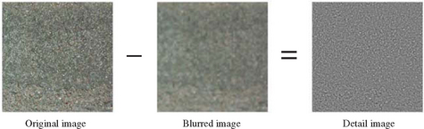
Once a blurred version of the high-resolution image has been created, the high-frequency components are extracted by subtracting the blurred image from the unprocessed one. The subtraction can be done using a subtractive blend mode, the accumulation buffer, or the appropriate texture environment function. The result is an image with signed color components that contains the high-frequency elements of the image. The input images must be scaled and biased so that the result of the subtraction is limited to the [0, 1] range, since negative pixel values will be clamped when the image is used as a texture. Checking the range of color values in the images makes it possible to maximize the range of the resulting subtracted image. If the implementation supports the imaging subset, the minmax function can be used to find the range of pixel values in both the high resolution and blurred copies of the detail texture image. The values can be used to scale and bias the inputs to the subtract operation to maximize the dynamic range of the resulting image. When the image is created, it should be biased so that the sum of the color values equals ![]() . This is necessary so that the detail texture will make no contribution when it’s minified.
. This is necessary so that the detail texture will make no contribution when it’s minified.
14.14 Texture Sharpening
Like detail textures, texture sharpening is another method for enhancing high-frequency detail on a magnified texture. Rather than creating a separate detail texture, however, texture sharpening augments high-frequency information by applying a sharpening operation to the texture similar to unsharp masking. This operation, a staple of image processing, increases the contrast of small details in the magnified texture. It has an advantage over detail textures in that is doesn’t require creating and applying a detail texture as a separate step. It does require that the magnified texture be mipmapped, since it combines multiple mipmap levels of the texture to create the sharpened image.
The sharpening operation computes the difference between the magnified finest level (level 0) and the next coarser level (level 1). A weighted version of the result is added to the magnified finest image to produce the sharpened result. The result is an extrapolation from the level 1 image to the level 0 image. The weighting factor applied to the difference, f, is a function of the magnification factor f(LOD). The equation to compute the texel color T from the top two texture levels and current magnification is:
where Tsharp is the new texel color, T0 is the magnified texel color at level 0, and T1 is the magnified texel color at level 1. The f(LOD) function takes an LOD value (which will be negative, since sharpening is only applied to magnified textures) and produces a weighting factor between 0 and 1. The resulting Tsharp color components are clamped to the range [0, 1]. Note that computing the T0 − T1 result is essentially the same technique used to create a signed intensity detail texture.
The texture sharpening functionality is available in some OpenGL implementations through the SGIS_sharpen_texture extension. Unfortunately, support for this extension is not widespread. At the time of this writing, there is no equivalent EXT or ARB extension, nor is texture sharpening supported as core functionality in any OpenGL specification. However, given the ability to approximate f(LOD) in a fragment program, the sharpening functionality can be readily implemented in the programmable pipeline.
Texture sharpening can be implemented at the application level using multitexture or multiple passes with the same caveats that apply to computing per-fragment values of f(LOD). If the LOD is constant across the polygon, the application can compute the constant f(LOD) value. One way to compute an approximate f (LOD) at each fragment is to create a mipmap texture with the values of f at each level. Texturing with this map generates a filtered version of f(LOD). The resulting image can be used as a weight within a multitexture operation or with framebuffer blending. Section 13.7.2 describes the steps in the LOD calculation in more detail. Section 12.3.2 describes a version of the extrapolation algorithm for still images using the accumulation buffer and framebuffer blending.
14.15 Mipmap Generation
OpenGL supports a modest collection of filtering algorithms, the highest quality filter being GL_LINEAR_MIPMAP_LINEAR, which does trilinear mipmapping. Mipmap filtering requires that the mipmap levels needed for filtering be loaded into texture memory. OpenGL does not specify a method for generating these individual mipmap level of details. Each level can be loaded individually; it is possible, but generally not desirable, to use a different filtering algorithm to generate each mipmap level. OpenGL 1.4 adds functionality to the pipeline to generate mipmaps automatically from the base level (GENERATE_MIPMAP), but does not precisely specify the filter algorithm.4
The OpenGL utility library (GLU) provides a simple command (gluBuild2DMipmaps) for generating all of the levels required for mipmapping a 2D or 1D texture. The algorithm employed by most implementations is a box filter. A box filter is a pragmatic choice; it is simple, efficient, and can be repeatedly applied to an LOD level to generate all coarser levels required in a mipmap. A frequency domain analysis shows, however, that the box filter has poor filtering characteristics, which can lead to excessive blurring and aliasing artifacts. A common example of these limitations occurs if a texture contains very narrow image features (such as narrow lines). Aliasing artifacts can be very pronounced in this case.
Although the limitations of box filtering are well known, finding the best mipmap filtering function is less obvious. The choice of filter is dependent on the manner in which the texture will be used and is somewhat subjective. The choice of filter is burdened with additional trade-offs if the mipmap must be generated at run time, and therefore must be filtered quickly. One possibility is the use of a bicubic filter—a weighted sum of 16 pixels for 2D images. Mitchell and Netravali (1988) propose a family of cubic filters for general image reconstruction which can be used for mipmap generation. The advantage of the cubic filter over the box filter is that the cubic filter can have negative side lobes (weights) which help maintain sharpness while reducing the image size. This can help reduce some of the blurring effect of filtering with mipmaps.
When crafting a new filtering algorithm for mipmap generation, it is important to keep a few guidelines in mind. To minimize accumulated error, the highest resolution (finest) image of the mipmap (level 0) should always be used as the input image source for each level to be generated. For the box filter, a particular level can be produced by repeating the filter to the results of the previous filtering operation. This works because the box filter can produce the correct result for a given level by using the preceding level as input. The filter parameters are independent of LOD level. This invariance is not always true for other filter functions. Each time a new (coarser) level is generated, the filter footprint may need to be scaled to four times its previous size.
Another constraint is that mipmap levels must maintain strict factor of two reductions in each dimension when filtering to a coarser level. Filters with input widths wider than two will be forced to sample outside the boundaries of the input image. Providing input values outside of the input image is commonly handled by using the value of the nearest edge pixel when sampling. This algorithm should be adjusted, however, if the mipmapped texture will be applied using the GL_REPEAT wrap mode. In this case, the levels will be filtered more accurately if sample values requested from outside the image should be wrapped to the appropriate texel from the opposite edge, effectively filtering from a repeating image.
While mipmaps can always be generated using the host processor, the OpenGL pipeline can be used to accelerate the process by performing the filtering operations. For example, the GL_LINEAR minification filter can be used to draw an image of exactly half the width and height of an image loaded into texture memory. This is done by drawing a rectangle with the appropriate transformation; it is sized so its pixel dimensions in screen space are exactly one half of the texture image’s dimensions. The rendered image produced has effectively been filtered to half of its dimensions using a box filter. The resulting image can then be read from the color buffer back to host memory for later use as a level. The read step can be eliminated and the the image can be copied directly into the texture using glCopyTexImage. If the implementation supports ARB_render_texture, even the copy step can be removed. The filtering process can be repeated using the newly generated mipmap level to produce the next level. The process can be continued until the coarsest level has been generated.
If the texture LOD extension SGIS_texture_lod (which became part of the core in OpenGL 1.2) is available, a further optimization to this process is possible. By clamping the mipmap to only the LOD levels that have been created, the mipmap can be built in place. The mipmap can be created with only level 0 in place. That level can be used to render an image for level 1, which can be used as the new texture source. This makes it possible to build up the mipmap texture without having to switch between two texture objects.
Although this method is very efficient, it is limited to creating new levels using the existing texture filters. There are other mechanisms within the OpenGL pipeline that can be used to produce higher-quality filtering. Convolution filtering can be implemented using the accumulation buffer (this discussed in detail in Section 12.6.2). An arbitrary filter kernel can be constructed using a special texture image applied to a rectangular geometry of the proper size and position. The texel color to be filtered is applied to geometry itself; the special texture modulates that color over the geometry. The accumulation buffer combines multiple passes with this technique to produce the final image. Combining point-sampled texturing with the accumulation buffer allows the application of nearly arbitrary filter kernels. This method does not handle the problem of sampling outside the image well, however, which limits its usefulness for wide filter kernels.
Convolution filters may also be implemented directly within fragment programs providing substantial flexibility in the types of filtering that can be performed within the pipeline. Typically custom fragment programs are written for each filter type. OpenGL implementations supporting the imaging subset also directly implement convolution operations in the pixel pipeline.
14.16 Texture Map Limits
Texture mapping is a versatile component for building graphics effects, but its very desirability can be its downside. It is common for an ambitious application to run into the limits to available texture memory. Most OpenGL implementations hardware accelerate texture mapping, but only if they are located within a finite texture memory storage area. OpenGL implementations often attempt to mitigate the finite size problem by virtualizing the texture memory resource. This allows an application to create an arbitrarily large set of texture maps; however, this virtualization isn’t free. As the texture memory resource becomes oversubscribed, performance will degrade. For the developer of an application that makes extensive use of texture, there is a tension between rationing available texture memory to maximize performance, and using texture lavishly to improve image quality.
The practical result of this limitation is that a well-designed application creates textures no larger than they need to be to meet image quality goals. An application designer needs to anticipate how textures will be used in each scene to determine the appropriate resolution to use. Using textures efficiently is always important. Where possible, images should be crafted to minimize wasted texels. For example, when faced with an image that doesn’t have power-of-two dimensions, the best choice is usually not simply rounding the texture size up to the next power-of-two. Besides such standard techniques as image tiling and mosaicing, many implementations support a special texture version that doesn’t require power-of-two dimensions. Vendor-specific extensions, such as NV_texture_rectangle and more widely adopted extensions such as ARB_texture_non_power_of_two, provide this functionality, although there are often limitations on the range of wrap modes or filtering that can be applied to such textures. Even the standard power-of-two dimension limitation doesn’t mean a texture has to be square. If a texture is typically used with an object that is projected to a non-square aspect ratio, then the aspect ratio of the texture can be scaled appropriately to make more efficient use of the available storage.
14.17 Summary
Texture mapping is undoubtedly the most powerful component in a graphics library. At least part of the reason is its ability to marry image-based and geometry-based processing with great flexibility. This chapter only provides a sampling of some of building block algorithms used to create sophisticated techniques. A survey of graphics “tricks and techniques” books, such as Graphics Gems (Goldman, 1990) and GPU Gems (Fernando, 2004), will reveal more ideas and are valuable references.
The best approach, however, is to have a through understanding of texture mapping. Nothing can replace a careful reading of the OpenGL core and extension specifications, augmented with some well-crafted test applications. With a deep understanding of OpenGL’s texture mapping capabilities, many opportunities for novel applications become apparent.