
GPU alignment of two and three sequences
J. Li; S. Ranka; S. Sahni University of Florida, Gainesville, FL, United States
Keywords
GPU; CUDA; Bioinformatics; Performance analysis; Sequence alignment
1 Introduction
1.1 Pairwise alignment
Sequence alignment is a fundamental bioinformatics problem. Algorithms for both pairwise alignment (ie, the alignment of two sequences) and the alignment of three sequences have been intensely researched deeply. In pairwise sequence alignment, we are given two sequences A and B and are to find their best alignment (either global or local). For DNA sequences, the alphabet for A and B is the 4 letter set {A, C, G, T} and for protein sequences, the alphabet is the 20 letter set {A, C−I, K−N, P−T, V WY}. The best global and local alignments of the sequences A and B can be found in O(|A|*|B|) time using the Needleman-Wunsch [1] and Smith-Waterman [2] dynamic programming algorithms. In this work, we consider only the local alignment problem, though our methods are readily extendable to the global alignment problem.
A variant of the pairwise sequence alignment problem asks for the best k, k > 0, alignments. In the database alignment problem, we are to find the best k alignments of a sequence A with the sequences in a database D. The database alignment problem can be solved by solving |D| pairwise alignment problems with each pair comprising A and a distinct sequence from D. This solution requires |D| applications of the Smith-Waterman algorithm.
When the sequences A and B are long or when the number of sequences in the database D is large, computational efficiency is often achieved by replacing the Smith-Waterman algorithm with a heuristic that trades accuracy for computational time. This is done, for example in the sequence alignment systems BLAST [3], FASTA [4], and Sim2 [5]. However, with the advent of low-cost parallel computers, there is renewed interest in developing computationally practical systems that do not sacrifice accuracy. Toward this end, several researchers have developed parallel versions of the Smith-Waterman algorithm that are suitable for graphics processing units (GPUs) [6–11]. The work of Khajej-Saeed et al. [9], Sriwardena and Ranasinghe [10], and Li et al. [12] is of particular relevance to us as this work specifically targets the alignment of two very long sequences, while the remaining research on GPU algorithms for sequence alignment focuses on the database alignment problem, and the developed algorithms and software are unable to handle very large sequences. For example, CUDASW++2.0 [8] cannot handle strings whose length is more than 70,000 on NVIDIA Tesla C2050 GPU.
As noted in Ref. [9], biological applications often have |A| in the range 104 to 105 and |B| in the range 107 to 1010. We refer to instances of this size as very large. Ref. [9] modified the Smith-Waterman dynamic programming equations to obtain a set of equations that were more amenable to parallel implementation. However, this modification introduced significant computational overhead. Despite this overhead, their algorithm was able to achieve a computational rate of up to 0.7 GCUPS (billion cell updates per second) using a single NVIDIA Tesla C2050. The instance sizes they experimented with had |A|*|B| up to 1011. Although Ref. [10] developed their GPU algorithms for pairwise sequence alignment specifically for the global alignment version, their algorithms are easily adapted to the case of local alignment. While their adaptations do not have the overheads of those of Ref. [9] that result from modifying the recurrence equations so as to increase parallelism, their algorithm is slower than that of Ref. [9]. The pairwise sequence alignment algorithms developed by Ref. [12] are currently the fastest GPU algorithms for very long sequences. We elaborate on these later in this chapter and benchmark these algorithms against those of Refs. [9, 10].
1.2 Alignment of Three Sequences
In the three-sequence alignment problem, we are given three sequences, S0, S1, and S2. We are to insert gaps into the sequences so that the resulting sequences are of the same length; in the resulting sequences, each character is said to be aligned with the gap or character in the corresponding position in each of the other sequences; and the alignment score is maximized. On a single-core CPU, the best alignment of the given three sequences (ie, the one with maximum score) can be found in O(|S0|*|S1|*|S3|) time using dynamic programming [13].
Several papers have been written on three-sequence alignment. We briefly mention a few here. Ref. [14] developed algorithms for the optimal alignment of three sequences using a constant gap weight. Ref. [15] developed algorithms to align three sequences using an affine gap penalty model. Ref. [16] reduced the memory requirement of these algorithms to be quadratic in the sequence length. Ref. [17] developed a faster three-sequence alignment algorithm using a speed-up technique based on Ukkonen’s greedy algorithm [18]. Ref. [19] used a position-specific gap penalty model for three-sequence alignment. Ref. [20] proposed a divide-and-conquer algorithm for three-sequence alignment, and Ref. [21] proposed a parallel algorithm for three-sequence alignment.
Besides being of interest in its own right, three-sequence alignment has been proposed as a base step in the alignment of a larger number of sequences. For example, Ref. [22] reported improved accuracy when three-sequence alignment was used instead of pairwise sequence alignment in their progressive multiple sequence alignment program aln3nn. Three-sequence alignment also helps in the tree alignment problem [23].
Two GPU algorithms to align three sequences were developed by Ref. [24]. These are described later in this chapter.
2 GPU architecture
The GPU algorithms described later in this chapter target the NVIDIA Tesla C2050 GPU, which is also known as Fermi. The C2050 has 14 streaming multiprocessors (SMs) and each SM has 32 streaming processors (SPs) giving the C2050 a total of 448 SPs or cores. Fig. 1 shows the architecture of a C2050 SM. Although each SP of a C2050 has its own integer, single- and double-precision units, the 32 SPs of an SM share 4 single-precision transcendental function units. An SM has 64 KB of on-chip memory that can be “configured as 48 KB of shared memory with 16 KB of L1 cache (default setting) or as 16 KB of shared memory with 48 KB of L1 cache” [25]. Additionally, there are 32K 32-bit registers per SM and 3 GB of off-chip device/global memory that is shared by all 14 SMs. The peak performance of a C2050 is 1288 GFlops (or 1.288 TFlops) of single-precision operations, and 515 GFlops of double-precision operations and the power consumption is 238 W [26]. Once again, the peak of 1288 GFlops requires that MADDs and SF instructions be dual-issued. When there are MADDs alone, the peak single-precision rate is 1.03 GFlops.
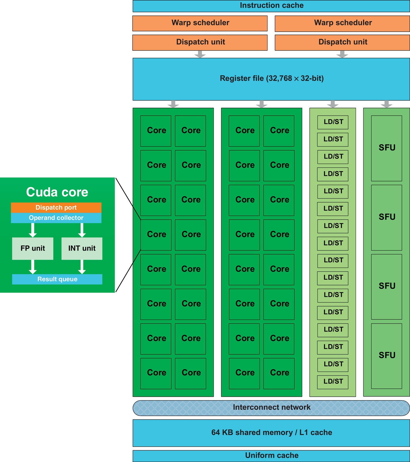
In NVIDIA parlance, the compute capability of the C2050 is 2.0. The key challenge in deriving high performance on CUDA GPUs is to be able to effectively minimize the memory traffic between the SMs and the global memory of the GPU. Data that is used repeatedly should go to registers or shared memory, while data that is used less frequently but of larger size should go to device memory.
3 Pairwise alignment
In this section, we describe the single-GPU parallelizations of the unmodified Smith-Waterman algorithm that were originally developed by us in Ref. [12]. These obtain a speedup of up to 17 relative to the single-GPU algorithm of Ref. [9] and a computational rate of 7.1 GCUPS. Our high-level parallelization strategy is similar to that used by Ref. [28, 29] to arrive at parallel algorithms for local alignment and syntenic alignment on a cluster of workstations, respectively. Both divide the scoring matrix into as many strips as there are processors, and each processor computes the scoring matrix for its strip row wise. Ref. [28] did the traceback needed to determine the actual alignment serially using a single processor, while Ref. [29] did the traceback in parallel using a strategy similar to the one we used. The essential differences between our work and that of Refs. [28, 29] are (a) our algorithms are optimized for a GPU rather than for a cluster, (b) we divide the scoring matrix into many more strips than the number of SMs in a GPU, and (c) the computation of a strip is done in parallel using many threads and the CUDA cores of an SM rather than serially.
3.1 Smith-Waterman Algorithm
Let A = a1a2…am and B = b1b2…bn be the two sequences that are to be locally aligned. Let c(ai, bj) be the score for matching or aligning ai and bj, and let α be the gap opening penalty and β the gap extension penalty. So the penalty for a gap of length k is α + kβ. Gotoh’s [30] variant of the Smith-Waterman dynamic programming algorithm with an affine penalty function uses the following three recurrences:
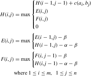
Here the score matrices H, E, and F have the following meaning:
1. H(i, j) is the score of the best local alignment for (a1…ai) and (b1…bj).
2. E(i, j) is the score of the best local alignment for (a1…ai) and (b1…bj) under the constraint that ai is aligned to a gap.
3. F(i, j) is the score of the best local alignment for (a1…ai) and (b1…bj) under the constraint that bj is aligned to a gap.
The initial conditions are H(0, 0) = H(i, 0) = H(0, j) = 0; ![]() ; E(i, 0) = −α − iβ;
; E(i, 0) = −α − iβ; ![]() ;
; ![]() ;
; ![]() ; F(0, j) = −α − jβ; 1 ≤ i ≤ m, 1 ≤ j ≤ n. The pseudocode is shown in Algorithm 1.
; F(0, j) = −α − jβ; 1 ≤ i ≤ m, 1 ≤ j ≤ n. The pseudocode is shown in Algorithm 1.

As mentioned in the introduction, the GPU adaptations of Refs. [9, 10] are most suited for the pairwise alignment of very long sequences. Ref. [9] enhanced parallelism by rewriting the recurrence equations. This rewrite eliminated the E terms and so their algorithm initially computed H values that differ from those computed by the original set of equations. Let ![]() be the computed H values. In a follow-up step, modified E values,
be the computed H values. In a follow-up step, modified E values, ![]() , were computed. The correct H values were then computed in a final step from
, were computed. The correct H values were then computed in a final step from ![]() and
and ![]() . Although the resulting three-step computation increased parallelism, it also increased I/O traffic between device memory and the SMs.
. Although the resulting three-step computation increased parallelism, it also increased I/O traffic between device memory and the SMs.
Ref. [10] proposed two GPU algorithms for global alignment using the Needleman-Wunsch dynamic programming algorithm [1]. These strategies can be readily deployed for local alignment using Gotoh’s variant of the Smith-Waterman algorithm. Both of the strategies of Ref. [10] are based on the observation that for any (i, j), the H, E, and F values depend only on values in the positions immediately to the north, northwest, and west of (i, j) (Fig. 2). Consequently, it is possible to compute all H, E, and F values on the same antidiagonal, in parallel, once these values have been computed for the preceding two antidiagonals. The first algorithm, Antidiagonal, of Ref. [10] does precisely this. The GPU kernel computes H, E, and F values on a single antidiagonal using values stored in device/global memory for the preceding two antidiagonals. The host program sends the two strings A and B to device memory and then invokes the GPU kernel once for each of the m + n − 1 antidiagonals. Additional (but minor) speedup can be attained by recognizing that the computation for the first and last few antidiagonals can be done faster on the host CPU and invoking the GPU kernel only for sufficiently large antidiagonals. When we want to determine the score of only the best alignment, the device memory needed by Antidiagonal is ![]() . However, when the best alignment also is to be reported, we need to save, for each (i, j), the direction (north, northwest, west) and the scoring matrices (H, E, F) that yielded the values for this position. O(mn) memory is required to save this information. Following the computation of the H, E, and F values, a serial traceback is done to determine the best alignment.
. However, when the best alignment also is to be reported, we need to save, for each (i, j), the direction (north, northwest, west) and the scoring matrices (H, E, F) that yielded the values for this position. O(mn) memory is required to save this information. Following the computation of the H, E, and F values, a serial traceback is done to determine the best alignment.

The second GPU algorithm, BlockedAntidiagonal, of Ref. [10] partitions the H, E, and F values into s × s square blocks (Fig. 3) and employs a GPU kernel to compute the values for a block. The host program allocates blocks to SMs, and each SM computes the H, E, and F values for its assigned block using values computed earlier and stored in device memory for the blocks immediately to its north, northwest, and west. Hence BlockedAntidiagonal attempts to enhance performance by utilizing both block-level parallelism and parallelism within an antidiagonal of a block. More importantly, it seeks to reduce I/O traffic to device memory and to utilize shared memory. Notice that device I/O is now needed only at the start and end of a block computation. The block assignment strategy of Fig. 3 does the computation in blocked antidiagonal order with the host invoking the kernel for all blocks on the same antidiagonal. The total number of blocks is O(mn/s2), and the I/O traffic between global memory and the SMs is O(mn). In contrast, the I/O traffic for Antidiagonal is O(mn). Experimental results reported in Ref. [10] demonstrate that BlockedAntidiagonal is roughly two times faster than Antidiagonal. Their research shows that BlockedAntidiagonal exhibits near-optimal performance when the block size s is 8. The BlockedAntidiagonal strategy of Fig. 3 may be enhanced for the case when we are interested only in the score of the best alignment. In this enhancement, we write to global memory only the computed values for the bottom and right boundaries of each block. This reduces the global memory I/O traffic to O(mn/s).

3.2 Computing the Score of the Best Local Alignment
In our GPU adaptation, StripedScore, of the Smith-Waterman algorithm, we assume that m ≤ n (in case this is not so, simply swap the roles of A and B) and partition the scoring matrices H, E, and F into ⌈n/s⌉m × s strips (Fig. 4). Here s is the strip width. Let p be the number of SMs in the GPU (for the C2050, p = 14). The GPU kernel is written so that SM i computes the H, E, and F values for all strips j such that j mod p = i, 0 ≤ j < ⌈n/s⌉, 0 ≤ i < p. Each SM works on its assigned strips serially from left to right. That is, if SM 0 is assigned strips 0, 14, 28, and 42 (this is the case, for example, when q = 14, s = 8, and n = 440), SM 0 first computes all H, E, and F values for strip 0, then for strip 14, then for strip 28, and finally for strip 42. When computing the values for a strip, the SM computes by antidiagonals confined to the strip with values along the same antidiagonal computed in parallel. The computed values for each antidiagonal are stored in shared memory. Each SM uses three one-dimensional arrays (preceding two antidiagonals and current antidiagonal) residing in shared memory and one for each of E and F and one for swapping purposes. The size of each of these arrays is ![]() . Additionally, each strip needs to communicate mH values and mF values to the strip immediately to its right. This communication is done via global memory. First, each strip accumulates, in a buffer, a threshold number, T, of H and F values needed by its right adjacent strip in shared memory. When this threshold is reached, the accumulated H and F values are written to global memory. The threshold T is chosen to optimize the total time. Each SM polls global memory to determine whether the next batch of H and F values it needs from its left adjacent strip are ready in global memory. If so, it reads this batch and computes the next T antidiagonals for its strip. If not, it waits in an idle state.
. Additionally, each strip needs to communicate mH values and mF values to the strip immediately to its right. This communication is done via global memory. First, each strip accumulates, in a buffer, a threshold number, T, of H and F values needed by its right adjacent strip in shared memory. When this threshold is reached, the accumulated H and F values are written to global memory. The threshold T is chosen to optimize the total time. Each SM polls global memory to determine whether the next batch of H and F values it needs from its left adjacent strip are ready in global memory. If so, it reads this batch and computes the next T antidiagonals for its strip. If not, it waits in an idle state.

Our striped algorithm therefore requires ![]() shared memory per SM and O(mn/s) global memory. The I/O traffic between global memory and the SMs is O(mn/s). To derive the computational time requirements (exclusive of the time taken by the global memory I/O traffic), we assume that the threshold value T is O(1). We note that the computation for the kth strip cannot begin until the top-right value of strip k − 1 has been computed. An SM with c processors takes Ta = O(s2/c) to compute the top-right value of the strip assigned to it and O(ms/c) time to complete the computation for the entire strip. So SM p − 1 cannot start working on the first strip assigned to it until time (p − 1)Ta. When an SM can go from the computation of one strip to the computation of the next strip with no delay, the completion time of SM p − 1, and hence the time taken by the GPU to do all its assigned work (exclusive of the time taken by global memory I/O traffic), is
shared memory per SM and O(mn/s) global memory. The I/O traffic between global memory and the SMs is O(mn/s). To derive the computational time requirements (exclusive of the time taken by the global memory I/O traffic), we assume that the threshold value T is O(1). We note that the computation for the kth strip cannot begin until the top-right value of strip k − 1 has been computed. An SM with c processors takes Ta = O(s2/c) to compute the top-right value of the strip assigned to it and O(ms/c) time to complete the computation for the entire strip. So SM p − 1 cannot start working on the first strip assigned to it until time (p − 1)Ta. When an SM can go from the computation of one strip to the computation of the next strip with no delay, the completion time of SM p − 1, and hence the time taken by the GPU to do all its assigned work (exclusive of the time taken by global memory I/O traffic), is ![]() =
= ![]() . When an SM takes less time to complete the computation for a strip than it takes to compute the data needed to commence on the next strip assigned to the SM (approximately,
. When an SM takes less time to complete the computation for a strip than it takes to compute the data needed to commence on the next strip assigned to the SM (approximately, ![]() ), an SM must wait
), an SM must wait ![]() time between the computation of successive strips assigned to it. So the time at which SM p finishes is
time between the computation of successive strips assigned to it. So the time at which SM p finishes is ![]() =
= ![]() . We see that while computation time exclusive of global I/O time increases as s increases, and global I/O time decreases as s increases. Our experiments in Section 3.4 show that for large m and n, the reduction in global I/O memory traffic that comes from increasing the strip size s more than compensates for the increase in time spent on computational tasks. Although using a larger strip size s reduces overall time, the size of the available shared memory per SM limits the value of s that may be used in practice.
. We see that while computation time exclusive of global I/O time increases as s increases, and global I/O time decreases as s increases. Our experiments in Section 3.4 show that for large m and n, the reduction in global I/O memory traffic that comes from increasing the strip size s more than compensates for the increase in time spent on computational tasks. Although using a larger strip size s reduces overall time, the size of the available shared memory per SM limits the value of s that may be used in practice.
In our GPU implementation of StripedScore, the substitution matrix is stored in the shared memory of each SM using 23 × 23 × size of(int) bytes. Additionally, each SM has an output buffer of length 32 for writing values on the boundary of each strip to global memory. This buffer takes 32 × size of(int) bytes. We also use 6 arrays of length ![]() each to hold the H values on 3 adjacent antidiagonals, E values and F values, and new E or F values to be swapped with old values. Another 1200 bytes are reserved by the CUDA compiler to store built-in variables and pass function parameters. The shared memory cache was configured as 48 KB shared memory and 16 KB L1 cache. So,
each to hold the H values on 3 adjacent antidiagonals, E values and F values, and new E or F values to be swapped with old values. Another 1200 bytes are reserved by the CUDA compiler to store built-in variables and pass function parameters. The shared memory cache was configured as 48 KB shared memory and 16 KB L1 cache. So, ![]() should be less than 1902. Since we are aligning very large sequences, we assume s < m. Hence s < 1902 for our implementation.
should be less than 1902. Since we are aligning very large sequences, we assume s < m. Hence s < 1902 for our implementation.
The following are some of the key differences between BlockedAntidiagonal and StripedScore:
1. BlockedAntidiagonal requires many kernel invocations from the host, while StripedScore requires just one kernel invocation. In other words, the synchronization of BlockedAntidiagonal is done on the host side, while in StripedScore the synchronization is done on the device side, which significantly reduces the overhead.
2. In BlockedAntidiagonal the assignment of blocks that are ready for computation to SMs is done by the GPU block scheduler, while in StripedScore the assignment of strips to SMs is programmed into the kernel code.
3. The I/O traffic of StripedScore is O(mn/s), while that of BlockedAntidiagonal is O(mn).
4. While for BlockedAntidiagonal near-optimal performance is achieved when s = 8, we envision much larger s values for StripedScore, which can be up to 1900. Consequently, there is greater opportunity for parallelism within a strip than within a block.
The preceding steps can lead to significant improvement in the overall performance.
3.3 Computing the Best Local Alignment
In this section, we describe three GPU algorithms for the case when we want to determine both the best alignment and its score.
3.3.1 StripedAlignment
With each position (u, v) of H, E, and F, we associate a start state, which is a triple (i, j, X), where (i, j) are the coordinates of the local start point of the optimal path to (u, v). This local start point is either a position in the current strip or a position on the right boundary of the strip immediately to the left of the current strip. X is one of H, F, and E and identifies whether the optimal path to (say) H(u, v) begins at H(i, j), F(i, j), or E(i, j). StripedAlignment is a three-phase algorithm. The first phase is an extension of StripedScore in which each strip stores, in global memory, not only the H and F values needed by the strip to its right but also the local start states of the optimal path to each boundary cell. For each boundary cell (u, v), three start states (one for each of H(u, v), F(u, v), and E(u, v)) are stored. So, for the four strips of Fig. 5, the boundary cells store, in global memory, the local start states of subpaths that end at the boundary cells (*, 4), (*, 8), (*, 12), and (*, 16). Additionally, we need to store the local start state and the end state for the overall best alignment. Since the highest H score is to (8, 9) and the local start state for H(8, 9) is (7, 8, H), (7, 8, H) is initially stored in registers and finally written along with (8, 9, H) to global memory. In Phase 1, the local start states for the optimal paths to all boundary cells (not just the boundary cells through which the overall alignment path traverses) are written to global memory.

In Phase 2, we serially determine, for each strip, the start state and end state of the optimal alignment subpath that goes through this strip. Suppose for our example in Fig. 5, we determine that the optimal alignment path comprises a subpath from (7, 8, H) to (8, 9, H), another subpath from (3, 4, F) to (7, 8, H), and one from (2, 3, H) to (3, 4, F).
Finally, in Phase 3, the optimal subpath for each strip the optimal path goes through is computed by recomputing the H, E, and F values for the strips the optimal alignment path traverses. Using the saved boundary H and F values, it is possible to compute the subpaths for all strips in parallel.
3.3.2 ChunkedAlignment1
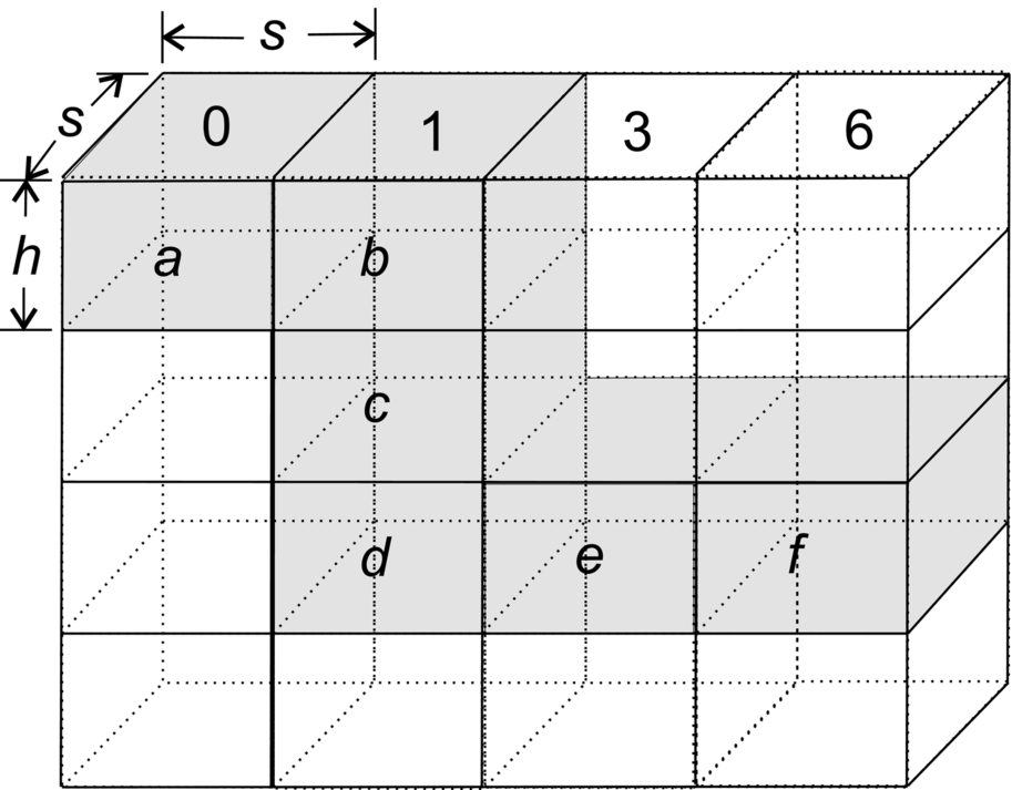
ChunkedAlignment1, like StripedAlignment, is a three-phase algorithm. In ChunkedAlignment1, each strip is partitioned into chunks of height h (Fig. 6). For each h × s chunk, we store, in global memory, the H, F, and local start states for positions on right vertical chunk boundaries (ie, vertical buffers, which are the same as boundary buffers in StripedAlignment) and the H and E values for horizontal buffers. The assignment of strips to SMs is the same as in StripedScore (and StripedAlignment).

In Phase 2, we use the data stored in global memory by the Phase 1 computation to determine the start and end states of the subpaths of the optimal alignment path within each strip. Finally, in Phase 3, the optimal subpaths are constructed by a computation within each strip through which the optimal alignment traverses. However, the computation with a strip can be limited to essential chunks, as shown by the shaded chunks in Fig. 6. The computation for these substrips can be done in parallel.
There are two major differences between StripedAlignment and Chunked Alignment1:
1. ChunkedAlignment1 generates more I/O traffic than does StripedAlignment and also requires more global memory on account of storing horizontal buffer data. Assuming that the height and width of the chunk are nearly equal, the I/O traffic and the global memory requirement are roughly twice the amount for StripedAlignment for the same strip size as the width of the chunk.
2. Unlike StripedAlignment, the computation begins at the start point of a chunk rather than at the first row of the strip. In practice, this should reduce the amount of computation significantly.
3.3.3 ChunkedAlignment2
ChunkedAlignmment2 is a natural extension of ChunkedAlignment1. Phase 1 is modified to additionally store, for the horizontal buffers, the local start state (local to the chunk) of the optimal path that goes through that buffer. Similarly, for vertical buffers the start state local to the chunk (rather than local to the strip) is stored. In Phase 2, we use the data stored in global memory during Phase 1 to determine the chunks through which the optimal alignment path traverses as well as the start and end states of the subpath through these chunks. In Phase 3, the subpath within each chunk is computed by using data stored in Phase 1 and the knowledge of the subpath end states determined in Phase 2. As was the case for StripedAlignment and ChunkedAlignment1, the subpaths for all identified chunks can be computed in parallel.
Unlike ChunkedAlignment1, additional computations and I/O need to be performed in Phase 1. The advantage is that the computation for all the chunks can be performed in parallel in Phase 3. So, for a given data set, if a large number of chunks corresponding to the shortest path are present in a given strip, this work will be assigned to a single SP for ChunkedAlignment1 and will effectively be performed sequentially. However, these chunks can potentially be assigned to multiple SPs. For example, in Fig. 6, strip 2 has three chunks. These will be assigned to the same SP using ChunkedAlignment1, but can be assigned to three different SPs using ChunkedAlignment2. Thus the amount of parallelism available is significantly increased.
3.3.4 Memory requirements
The code of Ref. [9] to find the actual alignment stores three m × n matrices in global memory. Since each matrix element is a score, each is a 4-byte int, so the code of Ref. [9] needs 12mn bytes of global memory. The code of Ref. [10] when extended to affine cost functions also needs 12mn bytes of global memory. The global memory required by our methods is instance-dependent. For each position encountered in Phase 3, we store direction information for all three matrices. For H, six possibilities exist for one cell, which are NEW (this cell starts a new alignment), DIAGONAL (this cell comes from diagonal direction), E_UP (this cell comes from the above cell in matrix E), H_UP (this cell comes from the above cell in matrix H), F_LEFT (this cell comes from the left cell in matrix F), and H_LEFT (this cell comes from the left cell in matrix H). Three bits are enough to store this information for each cell. For E, two possibilities exist, E_UP and H_UP. One bit is enough for this information. For F, one bit is enough to distinguish F_LEFT and H_LEFT. So, in the worst-case scenario, StripedAlignment requires 5mn/8 bytes of global memory while ChunkedAlignment1 and ChunkedAlignment2 require 5(ms + nh)/8 bytes. Hence StripedAlignment, for example, can handle problems with an mn value about 19 times as large as that handled by Refs. [9, 10]. Besides, when more memory space is required, Phase 3 can be split into multiple iterations. The same memory space required for one SM to compute part of the alignment within one strip can be reused in different iterations while computing for different strips.
3.4 Experimental Results
In this section, we present experimental results for scoring and alignment, respectively. All of these experiments were conducted on a NVIDIA Tesla C2050 GPU.
StripedScore
First, we measured the running time of StripedScore as a function of strip width s (Table 1 and Fig. 7). lenQuery is the length of the query sequence, and lenDB is the length of the subject sequence. As predicted in the analysis of Section 3.2, for sufficiently large sequences, the running time decreases as s increases. However, if sequences are relatively small, when s increases, the running time decreases first and then increases.

Table 1
Running Time (ms) of StripedScore for Different s Values
| lenQuery | 5103 | 10,206 | 20,412 | 30,618 | 51,030 |
| lenDB | 7168 | 14,336 | 28,672 | 43,008 | 71,680 |
| s = 64 | 67.2 | 260.2 | 1031.7 | 2316.7 | 6427.1 |
| s = 128 | 36.2 | 132.9 | 518.9 | 1161.4 | 3216.0 |
| s = 256 | 23.1 | 72.6 | 269.8 | 597.5 | 1645.2 |
| s = 512 | 22.3 | 50.1 | 160.9 | 344.9 | 932.3 |
| s = 1024 | – | 59.4 | 135.5 | 261.7 | 664.4 |
| s = 1900 | – | – | 175.0 | 279.9 | 625.7 |

Next we compared the relative performance of StripedScore with s = 1900, PerotRecurrence (the code of Ref. [9] modified to report the best score rather than the best 200 scores), BlockedAntidiagonal [10], EnhancedBA (our enhancement of BlockedAntidiagonal in which only the values on the right and bottom boundaries of each block are stored in global memory thus reducing global memory usage significantly), and CUDASW++2.0 [8]. Table 2 and Fig. 8 give the runtime for these algorithms. As can be seen, PerotRecurrence takes 13–17 times the time taken by StripedScore. The speedup ranges of StripedScore relative to BlockedAntidiagonal, EnhancedBA, and CUDASW++2.0 are, respectively, 20–33, 2.8–9.3, and 7.7–22.8. BlockedAntidiagonal and CUDASW++2.0 were unable to solve large instances because of the excessive memory they required.

Table 2
Running Time (ms) of Scoring Algorithms
| lenQuery | 1 × 10⁴ | 2 × 10⁴ | 3 × 10⁴ | 5 × 10⁴ | 1 × 10⁵ |
| lenDB | 1 × 10⁴ | 2 × 10⁴ | 3 × 10⁴ | 5 × 10⁴ | 1 × 10⁵ |
| PerotRecurrence | 815.3 | 1917.7 | 3061.7 | 7014.9 | 20,437.3 |
| StripedScore | 48.4 | 113.0 | 216.3 | 449.8 | 1543.1 |
| BlockedAntidiagonal | 957.2 | 3719.9 | – | – | – |
| EnhancedBA | 137.4 | 527.0 | 1185.9 | 3438.6 | 14,327.4 |
| CUDASW++2.0 | 374.5 | 1530.4 | 3404.0 | 10,259.1 | – |

StripedAlignment
For ease of coding, our implementation uses a char to store the direction information at each position encountered in Phase 3 rather than three bits as in the analysis of Section 3.3.4. We tested StripedAlignment with different s values, and the results are shown in Table 3 and Fig. 9. Using a similar analysis as used in Section 3.2, we determine the maximum strip size, which is limited by the amount of shared memory per SM, to be 410. The time for Phase 2 is negligible and is not reported separately. The time for all three phases generally decrease as s increases. For a really large s, the number of strips is comparable to or smaller than the number of SPs leading to idle time on some processors. Generally, choosing s = 256 gives the best overall performance for sequences of size up to 37,000. Choosing a larger s allows for larger sequences to be aligned (as I/O is inversely proportional to s).

Table 3
Running Time (ms) of StripedAlignment for Different s Values
| lenQuery | 10,430 | 15,533 | 20,860 | ||||||
| lenDB | 14,560 | 21,728 | 29,120 | ||||||
| Phase | 1 | 3 | Total | 1 | 3 | Total | 1 | 3 | Total |
| s = 64 | 616.9 | 440.1 | 1066.4 | 1352.9 | 973.5 | 2343.5 | 2402.4 | 1745.1 | 4176.5 |
| s = 128 | 328.6 | 298.9 | 633.5 | 707.4 | 650.2 | 1367.2 | 1245.4 | 1147.0 | 2408.1 |
| s = 256 | 183.9 | 318.0 | 505.6 | 384.0 | 715.7 | 1104.5 | 670.4 | 1273.5 | 1952.6 |
| s = 410 | 136.4 | 380.9 | 520.7 | 264.6 | 827.3 | 1096.0 | 484.2 | 1531.8 | 2020.9 |

We do not compare StripedAlignment with the algorithms of Refs. [8–10] for the following reasons (a) in Ref. [10], the traceback is done serially in the host CPU, (b) CUDASW++2.0 [8] does not have a traceback capability, and (c) the traceback of [9] is specifically designed for the benchmark suite SSCA#1 [31] and so aligns only multiple but small subsequences of length less than 128.
ChunkedAlignment1
There are two parameters in ChunkedAlignment1, s representing the width of one strip, and h representing the height of one chunk. Effectively, the scoring matrix is divided into blocks of size h×s. The data in Tables 4 through 6 show that, as was the case for StripedAlignment, performance improves as we increase s. Large values of h and s have the potential to reduce the amount of parallelism in Phase 3. A good choice from our experimental results is s = 410 and h = 128.
Table 4
Running Time (ms) of ChunkedAlignment1 (lenQuery = 10, 430 and lenDB = 14, 560)
| 64 | 128 | 256 | 410 | |||||||||
| Phase | 1 | 3 | Total | 1 | 3 | Total | 1 | 3 | Total | 1 | 3 | Total |
| 64 | 728.5 | 8.9 | 742.3 | 390.0 | 10.8 | 404.7 | 220.1 | 11.6 | 235.3 | 159.2 | 21.1 | 183.7 |
| 128 | 702.7 | 10.7 | 718.0 | 376.9 | 12.5 | 393.1 | 212.8 | 13.0 | 229.2 | 154.5 | 23.8 | 181.5 |
| 256 | 689.4 | 14.6 | 708.7 | 368.7 | 15.5 | 387.9 | 208.3 | 15.7 | 227.4 | 152.2 | 30.0 | 185.4 |
| 512 | 682.9 | 20.1 | 707.7 | 364.8 | 19.0 | 387.6 | 205.5 | 20.7 | 229.7 | 151.0 | 38.4 | 192.5 |
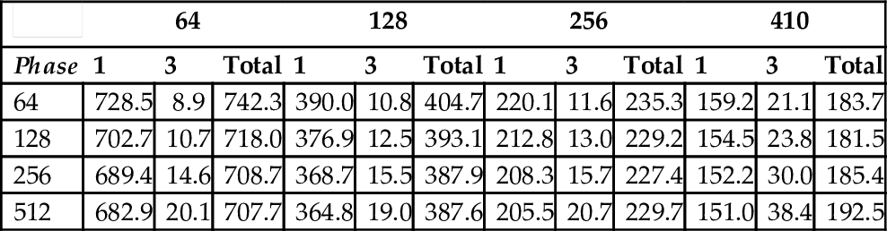
Table 5
Running Time (ms) of ChunkedAlignment1 (lenQuery = 15, 533 and lenDB = 21, 728)
| 64 | 128 | 256 | 410 | |||||||||
| Phase | 1 | 3 | Total | 1 | 3 | Total | 1 | 3 | Total | 1 | 3 | Total |
| 64 | 1596.6 | 13.1 | 1616.7 | 838.7 | 16.0 | 859.9 | 459.0 | 16.3 | 479.9 | 309.2 | 31.2 | 344.5 |
| 128 | 1540.4 | 15.9 | 1562.8 | 810.1 | 18.2 | 833.1 | 443.5 | 18.4 | 465.8 | 300.0 | 34.5 | 338.2 |
| 256 | 1511.3 | 21.6 | 1539.4 | 792.9 | 22.8 | 820.5 | 434.2 | 23.5 | 461.5 | 295.5 | 44.8 | 344.0 |
| 512 | 1497.0 | 30.3 | 1533.9 | 784.6 | 28.3 | 817.6 | 428.6 | 30.7 | 463.1 | 293.0 | 56.3 | 352.9 |

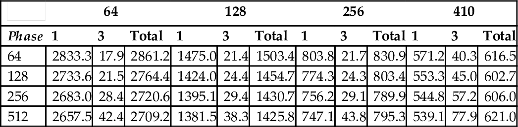
Table 6
Running Time (ms) of ChunkedAlignment1 (lenQuery = 20, 860 and lenDB = 29, 120)
| 64 | 128 | 256 | 410 | |||||||||
| Phase | 1 | 3 | Total | 1 | 3 | Total | 1 | 3 | Total | 1 | 3 | Total |
| 64 | 2833.3 | 17.9 | 2861.2 | 1475.0 | 21.4 | 1503.4 | 803.8 | 21.7 | 830.9 | 571.2 | 40.3 | 616.5 |
| 128 | 2733.6 | 21.5 | 2764.4 | 1424.0 | 24.4 | 1454.7 | 774.3 | 24.3 | 803.4 | 553.3 | 45.0 | 602.7 |
| 256 | 2683.0 | 28.4 | 2720.6 | 1395.1 | 29.4 | 1430.7 | 756.2 | 29.1 | 789.9 | 544.8 | 57.2 | 606.0 |
| 512 | 2657.5 | 42.4 | 2709.2 | 1381.5 | 38.3 | 1425.8 | 747.1 | 43.8 | 795.3 | 539.1 | 77.9 | 621.0 |
As expected, the Phase 3 time for ChunkedAlignment1 is significantly less than for StripedAlignment. Although this reduction comes with additional computational and I/O cost in Phase 1, the overall time for ChunkedAlignment1 is much less than for StripedAlignment. For sequences of size 20,860 and 29,120, the best time for StripedAlignment is 1952.6 ms, while that for ChunkedAlignment1 is 602.7 ms (s = 410, h = 128); the ratio is slightly more than 3.
The major advantage of ChunkedAlignment2 is better parallelism in Phase 3. However, the additional overhead in Phases 1 and 3 (in terms of I/O) result in performance that is slightly worse than that of ChunkedAlignment1, as shown in Tables 7–10 and Fig. 10. ChunkedAlignment2 is better than ChunkedAlignment1 only for strings in which, for the shortest distance, there are many chunks in one strip. For the strip sizes and the data sets that we used, we did not find this to be the case.
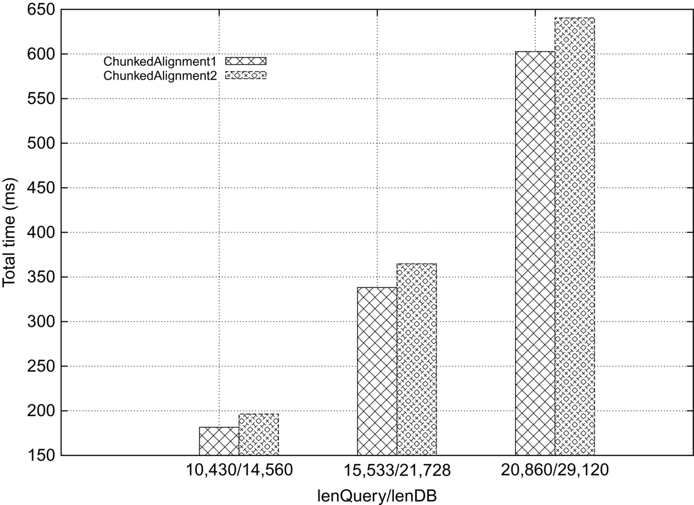
Table 7
Running Time (ms) of ChunkedAlignment2 (lenQuery = 10, 430 and lenDB = 14, 560)
| 64 | 128 | 256 | 410 | |||||||||
| Phase | 1 | 3 | Total | 1 | 3 | Total | 1 | 3 | Total | 1 | 3 | Total |
| 64 | 797.3 | 13.2 | 817.0 | 426.4 | 18.8 | 451.0 | 241.7 | 26.4 | 273.4 | 174.2 | 38.7 | 218.3 |
| 128 | 739.8 | 15.1 | 760.7 | 403.4 | 17.4 | 425.8 | 229.2 | 21.2 | 255.0 | 164.1 | 27.9 | 196.3 |
| 256 | 710.2 | 21.7 | 737.5 | 383.1 | 22.0 | 409.8 | 219.8 | 23.7 | 247.7 | 158.6 | 35.1 | 197.6 |
| 512 | 695.8 | 36.5 | 737.9 | 373.6 | 30.1 | 408.2 | 211.8 | 40.2 | 255.8 | 154.7 | 53.9 | 212.4 |

Table 8
Running Time (ms) of ChunkedAlignment2 (lenQuery = 15, 533 and lenDB = 21, 728)
| 64 | 128 | 256 | 410 | |||||||||
| Phase | 1 | 3 | Total | 1 | 3 | Total | 1 | 3 | Total | 1 | 3 | Total |
| 64 | 1745.0 | 19.6 | 1774.2 | 916.8 | 28.0 | 952.8 | 504.2 | 39.5 | 550.9 | 338.4 | 56.3 | 401.9 |
| 128 | 1619.8 | 22.6 | 1650.5 | 866.2 | 26.2 | 898.9 | 477.2 | 32.3 | 515.2 | 318.7 | 40.5 | 364.8 |
| 256 | 1555.6 | 32.8 | 1595.9 | 823.7 | 32.5 | 862.0 | 457.7 | 34.5 | 497.2 | 308.2 | 51.9 | 364.8 |
| 512 | 1524.0 | 55.8 | 1587.4 | 802.9 | 44.0 | 852.5 | 441.2 | 58.2 | 504.0 | 300.2 | 81.5 | 386.0 |

Table 9
Running Time (ms) of ChunkedAlignment2 (lenQuery = 20, 860 and lenDB = 29, 120)
| 64 | 128 | 256 | 410 | |||||||||
| Phase | 1 | 3 | Total | 1 | 3 | Total | 1 | 3 | Total | 1 | 3 | Total |
| 64 | 3105.7 | 1.6 | 3119.3 | 1612.1 | 37.6 | 1660.7 | 880.8 | 53.2 | 943.7 | 629.5 | 2.6 | 640.4 |
| 128 | 2886.5 | 1.7 | 2898.0 | 1521.3 | 35.0 | 1564.7 | 831.1 | 42.2 | 880.6 | 592.6 | 53.8 | 653.3 |
| 256 | 2762.9 | 43.6 | 2817.0 | 1449.4 | 43.7 | 1500.5 | 796.7 | 45.2 | 848.1 | 574.1 | 65.9 | 645.7 |
| 512 | 2706.2 | 73.6 | 2790.3 | 1413.3 | 58.1 | 1478.4 | 771.2 | 76.5 | 853.2 | 557.2 | 108.7 | 670.9 |

Table 10
Best Running Time (ms) of ChunkedAlignment1 and ChunkedAlignment2
| lenQuery/lenDB | 10,430/14,560 | 15,533/21,728 | 20,860/29,120 | ||||||
| Phase | 1 | 3 | Total | 1 | 3 | Total | 1 | 3 | Total |
| ChunkedAlignment1 | 154.5 | 23.8 | 181.5 | 300.0 | 34.5 | 338.2 | 553.3 | 45.0 | 602.7 |
| ChunkedAlignment2 | 164.1 | 27.9 | 196.3 | 318.7 | 40.5 | 364.8 | 629.5 | 2.6 | 640.4 |

Since StripedScore is an order of magnitude faster than PerotRecurrence and ChunkedAlignment1 is not an order of magnitude slower than StripedScore, we conclude, without experiment, that ChunkedAlignment1 is faster than the code of Ref. [9] modified to find the best alignment.
4 Alignment of three sequences
In this section, we describe two single-GPU algorithms for the optimal alignment of three sequences. These algorithms were originally presented by us in Ref. [24]. The first of these uses a layering approach, while the second uses a sloped approach. Experimental results using a NVIDIA GPU show that the sloped approach results in a faster algorithm and that this algorithm is an order of magnitude faster than a single-core alignment algorithm running on the host computer.
4.1 Three-Sequence Alignment Algorithm
The input to the three-sequence alignment problem is a set {S0, S1, S2} of three sequences and a substitution matrix sub such as BLOSUM [32] or PAM [33], which defines the score for character pairs xy. The output is a 3 × l matrix M where ![]() . Row i of M is Si, 0 ≤ i < 3, with gaps possibly inserted at various positions and such that each column of M has at least one nongap character. M defines an alignment whose score is
. Row i of M is Si, 0 ≤ i < 3, with gaps possibly inserted at various positions and such that each column of M has at least one nongap character. M defines an alignment whose score is

In this section, we define obj to be the sum-of-pairs function [13]:

The alignment M is optimal if it maximizes score(M). The dynamic programming algorithm to construct M first computes an (|S0| + 1) × (|S1| + 1) × (|S2| + 1) matrix H using the following recurrences [13]:
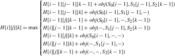
Here “−” denotes a GAP and β is the GAP penalty. The initial conditions are (i > 0, j > 0, k > 0):

The score of the optimal alignment is H[|S0|][|S1|][|S2|], and the corresponding alignment matrix M may be constructed using a backtrace process that starts at H[|S0|][|S1|][|S2|]. The time required to compute the H values is O(|S0||S1||S2|). An additional O(l) time is required to construct the optimal alignment matrix. The pseudocode to compute the optimal alignment score is shown in Algorithm 2.


4.2 Computing the Score of the Best Alignment
4.2.1 Layered algorithm
GPU computational strategy
In this algorithm, which is called LAY ERED, the three-dimensional matrix H is partitioned into s × s × (|S2| + 1) chunks (cuboids), as shown in Fig. 11, where s is an algorithm design parameter.

Let d be the number of chunks in the partitioning of H. These chunks form an (|S1| + 1)/s × (|S0| + 1)/s matrix whose elements may be numbered from 0 through d − 1 in antidiagonal (ie, top-right to bottom-left) order as in Fig. 11. Let p be the number of SMs in the GPU (for the C2050, p = 14). SM i of the GPU will compute the H values for all chunks j such that j mod p = i, 0 ≤ j < c, 0 ≤ i < p.
Each SM works on its assigned chunks serially. For example, when p = 3 and d = 12, SM 0 is assigned chunks 0, 3, 6, and 9. This SM will first compute the H values for chunk 0, then for chunk 3, then for chunk 6, and finally for chunk 9. In general, SM i computes chunk i, followed by i + p and so on.
The H values of a chunk are computed by the SM to which the chunk is assigned one layer at a time, where a layer is comprised of all H values in an s × s horizontal slice of the chunk. As can be seen, the total number of layers is |S2| + 1. Within a layer, the computations are done in antidiagonal order beginning with the antidiagonal that is composed of the top-left element of the layer (or slice). All values on the same antidiagonal of the layer are computed in parallel in a single instruction multiple data fashion. After one layer is computed, the SM moves to the next layer. After all layers are computed, the SM moves to the next chunk assigned to it. In order to achieve high performance, the computed H values for a layer are stored in the shared memory of the SM until the computation of the next layer is complete because the current layer’s H values are needed to compute those of the next layer. At any time during the computation, only two layers of H values are kept in shared memory, and the memory space for these two layers is used in a round-robin fashion to save shared memory.
From the dynamic programming recurrence for H, we see that the H values in a chunk depend only on those on the shared boundary (east vertical face) of the chunks to its west and northwest and those on the shared boundary (south vertical face) of the chunks to its north and northwest. With respect to the (|S1| + 1)/s × (|S0| + 1)/s matrix of chunks, it is necessary for the SM that computes the H values for chunk (i, j) to communicate the computed H values on its east vertical face to the SM that will compute the chunks (i, j + 1) and (i + 1, j + 1) (the top-left corner of this matrix is indexed (0, 0)), and the values on its south vertical face to the SM that will compute the chunks (i + 1, j) and (i + 1, j + 1). The s × (|S2| + 1)H values on each of these vertical faces are communicated to the appropriate SMs via the GPU’s global memory. Each SM writes the H values on its east and south faces to global memory. When an SM completes the computation for its current layer, it polls the global memory to determine whether the boundary values needed for the next layer are ready. If so, it proceeds to the next layer. If not, it idles. In case there is not a next layer in the current chunk, the SM proceeds to its next assigned chunk.
Analysis
To run the layered algorithm, each SM requires O(s2) shared memory to store the values associated with a layer and O(|S0||S1||S2|/s) global memory to communicate the H values on its east and south faces. Since shared memory is very small on current GPUs, the available shared memory constrains the chunk size s. Because of the high cost of data transfer between SMs and global memory (relative to the cost of arithmetic), the runtime performance of a GPU algorithm is often correlated to the volume of data transferred between the SMs and global memory. The layered algorithm transfers a total of O(|S0||S1||S2|/s) data between the GPU’s global memory and the SMs.
The computational time (excluding time taken by the global memory I/O traffic) is computed by first noting that the c cores of an SM can do the computation for one layer in O(s2/c) time computing the H values on each antidiagonal of a layer in parallel. So the time to do the computation for one chunk is O(s2|S2|/c). Since the computation for the ith chunk cannot begin until the first layers of its west, north, and northwest neighbor chunks have been computed, each SM, other than SM 0, experiences a startup delay. Because the antidiagonal from which the first chunk assigned to the last SM, SM p − 1, is ![]() , the startup delay for SM p − 1 is
, the startup delay for SM p − 1 is ![]() . When |S2| is sufficiently large (larger than
. When |S2| is sufficiently large (larger than ![]() ), SMs experience (almost) no further delay in working on their assigned SMs. The number of chunks assigned to an SM is O(|S0||S1|/(ps2)). So the total computation time (exclusive of global memory I/O time) is
), SMs experience (almost) no further delay in working on their assigned SMs. The number of chunks assigned to an SM is O(|S0||S1|/(ps2)). So the total computation time (exclusive of global memory I/O time) is ![]() .
.
While computation time exclusive of global I/O time increases as s increases (because the startup delay for SMs increases), global I/O time decreases as s increases. Our experiments show that for large |S0|, |S1|, and |S2|, the reduction in global I/O memory traffic that comes from increasing s is substantially higher than the increase in time spent on computational tasks. Thus, within limits, choosing a large s will reduce the overall time requirements. As noted earlier, the value of s is, however, upper-bounded by the amount of shared memory per SM.
4.2.2 Sloped algorithm
GPU computational strategy
In this algorithm, which is called SLOPED, we partition H into s × s × (|S2| + 1) chunks and assign these chunks to SMs as in the layered algorithm. However, instead of computing the H values in a chunk by horizontal layers and within a layer by antidiagonals, the H values are computed by “sloped” planes composed of H[i][j][k]s for which q = i + j + k is the same. The first sloped plane has q = 0, the next has q = 1, and the last has q = 2s + |S2|− 2. The computation for the plane q + 1 begins after that for the plane q completes. Within a plane q, the H values for all i, j, and k for which i + j + k = q can be done in parallel. The number of parallel steps in the computation of a chunk is therefore 2s + |S2|− 1. In contrast, the layered algorithm cannot compute all H values in a chunk’s layer in parallel. The computation of a layer is done by antidiagonals in 2s − 1 steps with each step computing the values on one antidiagonal in parallel. The total number of parallel steps employed by the layered algorithm in the computation of a chunk is (2s − 1) * (|S2| + 1). Hence when both the layered and sloped algorithms use the same s, the sloped algorithm uses fewer steps with each step encompassing more work that can be done in parallel. Under these conditions, the sloped algorithm is expected to perform better than the layered algorithm. However, as noted earlier, the value of s is constrained by the amount of local SM memory available. As we presently show, the sloped algorithm requires more SM memory and so must use a smaller s.
Analysis
To compute the H values on a sloped plane q, we need the H values from the planes q − 1, q − 2, and q − 3. For efficient computation, we must therefore have adequate SM memory for four sloped planes. Because a sloped plane may have up to (s+1)2H values, each SM must have sufficient memory to accommodate 4(s+1)2H values, which is twice the number of H values that the layered algorithm stores in the shared memory of an SM. The sloped algorithm generates the same amount of I/O traffic between the SMs and global memory as does the layered algorithm. The two algorithms also require the same amount of global memory.
Proceeding as for LAY ERED, we see that the delay time for SM p − 1 is ![]() where O(s3/c) is the time taken to compute the small pyramid. The time to compute all the chunks assigned to an SM is O(|S0||S1||S2|/(pc). So the total time (exclusive of global I/O traffic time) is
where O(s3/c) is the time taken to compute the small pyramid. The time to compute all the chunks assigned to an SM is O(|S0||S1||S2|/(pc). So the total time (exclusive of global I/O traffic time) is ![]() . Although the analysis shows the total time for SLOPED is larger than that for LAY ERED, because of the larger delay to start SM p − 1 when S0, S1, and S2 are large, the greater parallelism afforded by SLOPED coupled with the need for fewer synchronization steps dominates, and the measured runtime is smaller for SLOPED.
. Although the analysis shows the total time for SLOPED is larger than that for LAY ERED, because of the larger delay to start SM p − 1 when S0, S1, and S2 are large, the greater parallelism afforded by SLOPED coupled with the need for fewer synchronization steps dominates, and the measured runtime is smaller for SLOPED.
4.3 Computing the Best Alignment
The layered and sloped algorithms may be extended to compute not only the score of the best alignment but also the best alignment. We describe three possible extensions for the layered algorithm. These extensions represent a tradeoff among conceptual and implementation simplicity, computational requirements for the traceback done to compute the best alignment from the scores, and the amount of parallelism. Identical extensions may be made to the sloped algorithm.
4.3.1 LAY ERED-BT1
To compute the best alignment, we need to maintain additional information that can be used during the traceback. In particular, for each position (i, j, k) of H, we associate the coordinates (is, js, ks) of the local start point of the optimal path to (i, j, k). This local start point is a position on the boundary of north, northwest, or west neighbor chunk of the chunk that contains the position (i, j, k). LAY ERED-BT1 is a three-phase algorithm, as shown here:
1. Phase 1: This is an extension of LAY ERED in which each chunk stores, in global memory, not only the H values needed by its neighboring chunks but also the local start point of the optimal path to each boundary cell.
2. Phase 2: For each chunk, we sequentially determine the start point and end point of the subpath of the best alignment that goes through this chunk. This is done by tracing the best path backward from position (|S0|, |S1|, |S2|) to position (0, 0, 0) using the local start points of boundary cells computed in Phase 1. This traceback goes from the boundary of one chunk to the boundary of a neighbor chunk without actually entering any chunk.
3. Phase 3: The subpath of the best path within each chunk is computed by recomputing the H values for the chunks through which the best alignment path traverses. Note that Phase 2 determines which chunks the best path goes through. Using the saved boundary H values, it is possible to compute the subpaths for all chunks in parallel.
The global memory required by LAY ERED-BT1 is more than that required by LAY ERED because Phase 1 stores a 3D position with H value saved. Assuming 4 bytes for each coordinate of a 3D position and 4 bytes for an H value, LAY ERED-BT1 requires 16 bytes per boundary cell, while LAY ERED requires only 4. Additionally, in the Phase 3 computation, with every position in a chunk, we need to store which of the seven options on the right-hand side of the dynamic programming recurrence for H resulted in the max value. This can be done using 3 bits (or more realistically, 1 byte) per position in a chunk.
4.3.2 LAY ERED-BT2
Although LAY ERED-BT2 is also a three-phase algorithm, LAY ERED-BT2 partitions each chunk into subchunks of height h (Fig. 12). The three phases are as follows:
1. Phase 1: Chunks are assigned to SMs as in LAY ERED. In addition to the H and local start points stored in global memory by LAY ERED-BT1, we store the H values of the positions on the bottom face of each subchunk.
2. Phase 2: Use the local start point data stored in global memory by the Phase 1 computation to determine the start and end points of the subpaths of the best alignment path within each chunk. This phase computes the same start and end points as computed in Phase 2 of LAY ERED-BT1.
3. Phase 3: The subpath of the best path within each chunk is computed by recomputing the H values for the chunks through which the best alignment path traverses. For each chunk through which this path passes, the computation begins at the first layer of the topmost subchunk through which the path passes (Fig. 12, shaded subchunks are the subchunks through which the best alignment path passes). The computation for the different chunks through which the best alignment path passes can be done in parallel as in LAY ERED-BT1.
The major differences between LAY ERED-BT1 and LAY ERED-BT2 are as follows:
1. Since LAY ERED-BT2 saves H values on the bottom face of each subchunk in addition to data saved by LAY ERED-BT1, it generates more I/O traffic than LAY ERED-BT1 and also requires more global memory. The amount of additional I/O traffic and global memory required is O(S1||S2||S3|/h).
2. For each chunk through which the best alignment path passes, LAY ERED-BT1 begins the Phase 3 computations at layer 1 of that chunk while LAY ERED-BT2 begins this computation at the first layer of the topmost subchunk through which this path passes.
4.3.3 LAY ERED-BT3
For LAY ERED-BT3, the local start points are defined to be positions on neighboring subchunks of the subchunk that contains the position (i, j, k) (rather than points on neighboring chunks of the chunk that contains (i, j, k)). Here are the three phases of LAY ERED-BT3:
1. Phase 1: Chunks are assigned to SMs as in LAY ERED. For each subchunk, we store in global memory, the H values on its south, east, and bottom faces as well as the local start point of the optimal path to each of the positions on these faces.
2. Phase 2: For each subchunk, we sequentially determine, the start point and end point (if any) of the subpath of the best alignment path that goes through this subchunk.
3. Phase 3: The subpath (if any) of the best path within each subchunk is computed by recomputing the H values for those subchunks through which the best alignment path traverses. Note that Phase 2 determines the subchunks through which the best path goes. Using the saved boundary H values, it is possible to compute the subpaths for all subchunks in parallel.
LAY ERED-BT3 has more global I/O traffic than LAY ERED-BT2 in Phase 1 and also requires more global memory. Phase 2 of both algorithms do the same amount of work. We expect Phase 3 of LAY ERED-BT3 to be faster than that of LAY ERED-BT2 because of better load balancing resulting from the finer granularity of the per-subchunk work and the fact that there are more subchunks than chunks, which leads to more parallelism. For example, suppose one chunk has 50 subchunks through which the best alignment path passes and another chunk has only 1 such subchunk. Phase 3 of LAY ERED-BT2 can use at most 2 SMs with 1 working on all 50 subchunks of the first chunk and the other working on the single subchunk of the second chunk. The workload over the two assigned SMs is unbalanced and the degree of parallelism is only two. Phase 3 of LAY ERED-BT3, however, is able to use up to 51 SMs assigning 1 subchunk to each SM resulting in better workload balancing and a higher degree of parallelism.
4.4 Experimental Results
We benchmarked the GPU three-sequence alignment algorithms against a single-core algorithm running on the host machine, which had an Intel i7-980x 3.33 GHz CPU and 12 GB DDR3 RAM.
4.4.1 Computing the score of the best alignment
We fixed s = 67 for LAY ERED and s = 47 for SLOPED and experimented with real instances of different sizes. These two s values were determined from our experimental results that produced the least running time. The sequences used were retrieved from NCBI Entrez Gene [34], and their sizes are represented as a tuple (|S0|, |S1|, |S2|). The running time is shown in Table 11. The running time of the single-core scoring method and the single-core traceback method running on our host CPU is referred to as Scoring and Traceback in Table 11, respectively, for comparison purpose. As can be seen, SLOPED is about three times as fast as LAY ERED for large instances and is up to 90 times as fast as the single-core CPU algorithm! In our tests speedup increases with instance size.

4.4.2 Computing the alignment
Because of memory limitations, our scoring algorithms can handle sequences whose size is up to approximately (2500, 2500, 2500), while our alignment algorithms can handle sequences of size up to approximately (1500, 1500, 1500). We used s = 47, h = 40 for layered algorithms and s = 31, h = 100 for the sloped algorithms that were determined by experiments to be the optimal values.
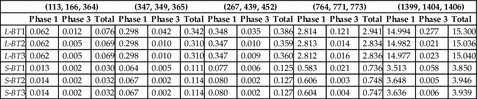
We tested our alignment algorithms, set with the preceding parameters, on the real instances used earlier for the scoring experiments. The measured runtimes are reported in Table 12 and Fig. 13 (L- for LAY ERED, S- for SLOPED). We do not report the time for Phase 2 because it is negligible compared to that for the other phases. Although BT2 and BT3 reduce the runtime of the third phase, the overall time is dominated by that for Phase 1. Again, the SLOPED algorithms are about three times as fast as the LAY ERED algorithms. The SLOPED algorithms provide a speedup between 21 and 56 relative to the single-core algorithm running on our host CPU.

Table 12
Running Time (s) of Traceback Methods for Real Instances
| (113, 166, 364) | (347, 349, 365) | (267, 439, 452) | (764, 771, 773) | (1399, 1404, 1406) | |||||||||||
| Phase 1 | Phase 3 | Total | Phase 1 | Phase 3 | Total | Phase 1 | Phase 3 | Total | Phase 1 | Phase 3 | Total | Phase 1 | Phase 3 | Total | |
| L-BT1 | 0.062 | 0.012 | 0.076 | 0.298 | 0.042 | 0.342 | 0.348 | 0.035 | 0.386 | 2.814 | 0.121 | 2.941 | 14.994 | 0.277 | 15.300 |
| L-BT2 | 0.062 | 0.005 | 0.069 | 0.298 | 0.010 | 0.310 | 0.347 | 0.010 | 0.359 | 2.813 | 0.014 | 2.834 | 14.982 | 0.021 | 15.036 |
| L-BT3 | 0.062 | 0.005 | 0.069 | 0.298 | 0.010 | 0.310 | 0.347 | 0.009 | 0.360 | 2.812 | 0.016 | 2.836 | 14.977 | 0.023 | 15.040 |
| S-BT1 | 0.013 | 0.002 | 0.030 | 0.064 | 0.005 | 0.111 | 0.077 | 0.006 | 0.125 | 0.583 | 0.021 | 0.736 | 3.513 | 0.058 | 3.850 |
| S-BT2 | 0.014 | 0.002 | 0.032 | 0.067 | 0.002 | 0.114 | 0.080 | 0.002 | 0.127 | 0.606 | 0.003 | 0.748 | 3.648 | 0.005 | 3.946 |
| S-BT3 | 0.014 | 0.002 | 0.032 | 0.067 | 0.002 | 0.114 | 0.080 | 0.002 | 0.127 | 0.604 | 0.004 | 0.747 | 3.636 | 0.006 | 3.939 |
5 Conclusion
GPUs are well suited to solve bioinformatics problems such as sequence alignment. However, performance is very dependent on the strategy used to map the underling serial algorithm to the GPU. For example, our GPU parallelizations of the unmodified Smith-Waterman algorithm for pairwise sequence alignment, StripedScore, achieves a speedup of 13–17 relative to the GPU algorithm of Ref. [9]. The speedup ranges relative to BlockedAntidiagonal [10] and CUDASW++2.0 [8] are, respectively, 20–33 and 7.7–22.8. Our algorithms achieve a computational rate of 7.1 GCUPS on a single GPU.
The sloped scoring algorithm for three-sequence alignment, which is three times as fast as the layered algorithm, provides a speedup of up to 90 relative to a single-core algorithm running on our host CPU. The sloped alignment algorithm is also three times as fast as the layered one and provides a speedup between 21 and 56 relative to the single-core algorithm.
As demonstrated in this chapter, GPUs have the potential to provide orders of magnitude speedup over the host CPU.