
Power management of mobile GPUs
T. Mitra; A. Prakash; A. Pathania* National University of Singapore, Singapore, Singapore
Abstract
The graphics processing units (GPUs) in mobile devices have come a long way in terms of their capabilities to accelerate both graphics- and general-purpose applications. However, they also consume a significant amount of power when executing such applications. This necessitates sophisticated power management techniques for the GPUs in order to save power and energy in mobile devices that typically have limited power budget and battery capacity.
In this chapter, we first discuss the advantages and limitations of the state-of-the-art power management techniques for both gaming- and general-purpose applications running on GPUs. In particular, existing approaches suffer from lack of coordination in power management between the central processing unit (CPU) and the GPU coinciding on the same chip in the mobile application processors. We present our recently proposed power management solutions to address these shortcomings through synergistic CPU-GPU execution and power management. Finally, we identify and elaborate on the open problems that provide further opportunities for reduction in power consumption of mobile GPUs.
Keywords
Low power; Mobile GPU; GPGPU; OpenGL; OpenCL; Mobile games
Acknowledgments
This work was partially supported by Singapore Ministry of Education Academic Research Fund Tier 2 MOE2012-T2-1-115 and CSR research funding.
1 Introduction
The system-on-chip (SoC) for mobile devices initially contained only a central processing unit (CPU), which would be considered very rudimentary by today’s standard. As the CPUs became more capable over time, they also started rendering graphic applications (mostly games) by a process known as “software rendering.” The CPU being designed for execution of sequential workloads was both performance-wise and power-wise inefficient when processing highly parallel graphic workloads. Nvidia introduced the first graphics processing unit (GPU) named SC10 [1] for mobile devices in 2004. GPUs were later etched on the same die as the CPUs leading to the emergence of heterogeneous multiprocessor system-on-chips (HMPSoCs) [2]. Since then GPUs have continued to improve and in the process transformed the mobile landscape. For example, Fig. 1 shows how much mobile gaming has advanced over the years, from one of the first mobile games Tetris released in 1989 for Nintendo Gameboy devices to Need for Speed No Limit released in 2015 for Android devices.

This performance came at the price of high power consumption. At time of this writing, one of the most advanced HMPSoCs available is Samsung’s Exynos 7 Octa (7420) fabricated on 14 nm technology. The ARM Mali-760 GPU in this HMPSoC with eight cores can consume up to 6 W of power when operating at the highest frequency level, comparable to 7 W consumed by the octa-core ARM big.Little CPU on the same chip [3]. A mobile device is battery powered and high power consumption can quickly drain its limited-capacity battery [4]. High power consumption also leads to high die temperature, which can cause permanent damage to the mobile device given its restricted heat dissipation capacity [5]. Inevitably, many power management technologies, such as digital voltage and frequency scaling (DVFS) and dynamic power management (DPM), that are available for PC-class GPUs have now made their way to mobile GPUs [3].
DVFS scales the frequency (and voltage) of the GPU to reduce its power consumption. GPU consumes less power at lower frequencies but also provides less performance. DVFS thereby allows a power-performance trade-off. DPM allows idle cores of the GPU to be power-gated eliminating their idle power consumption. The operating system (OS) subroutines that use DVFS and/or DPM to reduce power consumption of devices are called “governors.”
HMPSoCs, though similar in purpose to PC-class CPU-GPU systems, differ significantly in their architecture. Fig. 2 shows the abstracted block diagrams for both architectures. CPU and GPU are fabricated on separate dies in PC-class CPU-GPU systems, while in HMPSoCs they are on the same die. CPU and GPU have a different independent power supplies in PC-class CPU-GPU systems, while in HMPSoCs they share the power supply. Finally, CPU and GPU have their own private last-level memories (DRAM and graphics DRAM, respectively), while the last level memory is shared by them in HMPSoCs.

In addition to architecture, PC-class CPU-GPU systems also differ significantly in the management goals for their governors compared to the HMPSoCs. PC-class CPU-GPU systems are several times larger in size than HMPSoCs and are often accompanied by sophisticated cooling systems. They are also connected to a power supply and hence face no energy or thermal concerns. Governors designed for these systems mostly fixate on extracting maximum performance. On the other hand, HMPSoCs, being limited by their battery and cooling capacity, need their governors to provide acceptable performance in an energy/power-efficient fashion with no thermal violation. In HMPSoC, CPU and GPU share a common power budget called thermal dissipation power (TDP). Combined CPU and GPU power should not exceed beyond TDP. Without external cooling, TDP of most mobile platform is only 2–4 W, whereas the Exynos HMPSoC mentioned earlier (Samsungs Exynos 7 Octa 7420) can consume up to 13 W when both CPU and GPU are operating at their peak capacity.
The initial role for GPU in mobile devices was to unburden the CPU from the graphic processing for games. The ability to process highly parallel graphic workloads in a power-efficient manner turned out to be perfect for handling highly parallel general-purpose mobile workloads such as vision and image processing. Mobile GPUs also have now become sophisticated enough to run general-purpose computation on graphics processing unit (GPGPU) applications, similar to their PC-class counterparts. This capability allows them to help the CPU in tasks such as voice recognition and image processing, and even more interestingly opens up the possibility for large numbers of HMPSoCs to be put together to form low-power servers. Though GPU processing is similar for both games and GPGPU applications, the roles CPU plays in them are completely different.
While executing games, CPU and GPU need to work synergistically. Games use CPU for the general-purpose computation, for example, game physics and artificial intelligence (AI), while GPU is used for parallel 2D/3D graphics rendering. For games, CPU and GPU are in a producer-consumer relationship. To produce a game frame, the CPU first generates a frame, which it then passes on to the GPU for rendering. Games are also highly dynamic workloads that can change its requirements unpredictably depending on changes in the complexity of the scene being rendered. Thus games require a lightweight online governor that synchronously manages both the CPU and the GPU. In addition, being inherently user-interactive, games vary extensively from each other and provide infinite different paths of execution. As a result, profiling them a priori for power management is not viable.
On the other hand, in GPGPU applications, CPU and GPU act either as competitors or collaborators because a workload can be executed on any of them or both of them in parallel. Some workloads work better on CPU, while others work better on GPU, and for some both CPU or GPU are equally viable. Therefore GPGPU applications subject the system to an additional challenge of efficient workload partitioning among CPUs and GPUs. The behaviors of GPGPU applications are also mostly static; therefore an offline algorithm can be sufficient for the partitioning of workloads between CPU and GPU.
Linux or Android OS, which HMPSoCs often come installed with, comes with a set of default governors for CPU [6]. Among the default governors, Conservative is the governor designed for attaining power-efficiency on the CPU. Conservative is a general-purpose application agnostic governor that works on system-defined thresholds to perform DVFS. It increases or decreases CPU frequency by a step of freq_step when CPU utilization is above up_threshold or below down_threshold, respectively. The interval at which CPU utilization is measured is defined by sampling_down_factor. On the other hand, GPU DVFS is performed by a closed-source GPU driver, and it is not known what governor (or algorithm) the driver employs.
The separate CPU and GPU governor approach that Linux employs lacks synergy and does not reflect the complex interrelationships they have when executing games or GPGPU workloads. The problem, however, has been addressed in recent research in the form of specialized gaming or GPGPU governors. In this chapter, we characterize gaming and GPGPU workloads and present some of the current state-of-the-art governors designed for them. Finally, we discuss some of the open research problems that provide opportunities for further reduction in power consumption of a mobile GPU.
2 GPU Power Management for Mobile Games
We first measure the power consumption while executing gaming workloads on an Odroid XU+E board with Exynos 5 Octa (5410) HMPSoC as shown in Fig. 3. Exynos 5 Octa (5410) HMPSoC combines a powerful quad-core Cortex-A15 CPU with a sophisticated tri-core PowerVR SGX544 GPU. Both CPU and GPU support DVFS but neither CPU nor GPU can perform DPM. In the Samsung Exynos series HMPSoCs, DPM arrived in CPU and GPU with the introduction of Exynos 5 Octa (5422) and Exynos 7 Octa (7420), respectively [3].

As expected, the games turn out to be extremely power hungry. Fig. 4 shows the average power consumption of some of the latest mobile games, while running at peak performance with the highest CPU-GPU frequency setting. Fig. 4 shows that the games use both CPU and GPU for execution. Still some games consume more CPU power, while others consume more GPU power. This is indicative of substantial variation in the workloads that different games produce and the challenges involved in their power management.

We begin by describing some of the state-of-the-art gaming governors proposed in research. We then present our in-depth characterization of mobile gaming workloads, followed by details of our approach to reducing the power consumption of mobile games running on HMPSoCs.
2.1 State-of-the-Art Techniques
Power consumption during mobile gaming was a concern even before HMPSoCs were introduced [7]. Early works [8, 9] focused on reducing power consumption of a mobile CPU running open-source games through software rendering. These works are now obsolete as the introduction of mobile GPUs radically changed the way the games are executed on current mobile devices. Furthermore, most of the games played today are closed-source games. Therefore, in this section, we present details of only those works that can be applied to closed-source games running on HMPSoCs.
Texture-directed gaming governor
Sun et al. [10] show that there is a strong positive correlation between the texture operations performed on a CPU with rendering operations performed on a GPU in a HMPSoC. Based on this observation, the authors present a gaming governor that sets the frequency of the GPU reactively based on the texture processing load that a game places on the CPU.
Texture processing load is calculated from the number of times a call is made to the OpenGL function glBindTexture () by the game. The call count of this function showed a strong correlation of 0.87 with GPU utilization in six games. The gaming governor they propose calculates the texture processing load for each frame and then sets GPU frequency for the next frame based on a load-frequency table. The governor is provided with a load-frequency table for each playable scene in the game. The values in load-frequency tables are empirically determined and fine-tuned manually.
This gaming governor was evaluated on an Exynos 4 Quad (4412) HMPSoC and reduces power consumption of the GPU by 7.16% on an average for six games. It performed best on GPU-intensive games with high workload variations.
Control-theoretic gaming governor
Kadjo et al. [11] presented a gaming governor based on control theory. They model the CPU-GPU interaction in HMPSoC as a queuing system. Their proposed governor uses a multiinput multioutput state space controller to perform CPU-GPU DVFS in the queuing system so as to achieve a target frame rate for a game.
There are two queues in the system. The first queue is between the CPU and the GPU, while the second queue is between the GPU and the display. CPU injects the work in CPU-GPU queue, which is ejected by the GPU. The injection rate in CPU-GPU queue is determined by CPU frequency, while the ejection rate is determined by GPU frequency. Similarly, the GPU acts as an injector in the GPU-display queue, and the display acts as an ejector. Injection rate in GPU-display queue is determined by GPU frequency, while ejection rate is determined by the display’s refresh rate. The controller takes a game’s frame rate as an input parameter and ensures that there is sufficient work in both queues at all times by adjusting injection and ejection rates using CPU-GPU DVFS to prevent any stall.
This control-theoretic gaming governor was implemented on Intel Baytrail HMPSoC. The governor operated at a granularity of 50 ms and achieves an average power savings of 20% and 17% on the CPU and GPU, respectively.
Regression-based gaming governor
We presented a regression-based gaming governor in Ref. [12]. In our work [13], we extensively characterized the producer-consumer relationships between CPU and GPU when games are executed on an HMPSoC. Based on this characterization, we developed a power-performance model using linear regression and employed this model to drive CPU-GPU DVFS to run a game at target performance with minimal power consumption. We cover this governor in detail in this chapter.
2.2 CPU-GPU Relationship
The performance of a game is measured in frames per second (FPS). To produce a frame, the game requires both CPU and GPU to perform substantial calculations. CPU performs the game’s physics and AI-associated calculations based on which location of objects in a playable 3D scene is generated. This information is then sent to GPU for processing that creates a 2D image (frame) from the 3D scene, visually reflecting the current state of the scene. The frame produced by the GPU is then displayed on the screen.
Fig. 5 shows a simplified abstraction of how a game’s code is written. In the code, there is a one major loop that performs most of the processing. CPU’s part of the code is performed first, followed by GPU’s part of the code in the loop. Each iteration of the loop produces a single frame for the game. Fig. 5 clearly shows the producer-consumer relationship between CPU and GPU. Until CPU finishes processing a frame, GPU cannot start frame processing. Similarly, until GPU finishes processing the last frame, CPU cannot start processing the next frame.

CPU’s part of a game’s code works on real-system clock time, and an object in the game will always behave similarly on the screen in a given time interval irrespective of how fast the game loop executes (provided no user interaction happens in between and game code is deterministic). But, if the loop executes faster, then more frames are produced to reflect the behavior of the object. For example, Fig. 5 shows movement of a ball from points A to B separated by a distance of 100 pixels on the display. Assume that the ball is moving at 100 pixels/s. If the loop runs at 100 ms, then the movement of the ball will be shown to the user using 10 frames in a second. If the same loop runs at 200 ms, then the ball’s movement will be displayed using 5 frames in a second. Understandably, quality of service (QoS) experienced by the user will be superior in 10 FPS than 5 FPS as the user will visually perceive a smoother animation.
2.3 Power-Performance Trade-Off
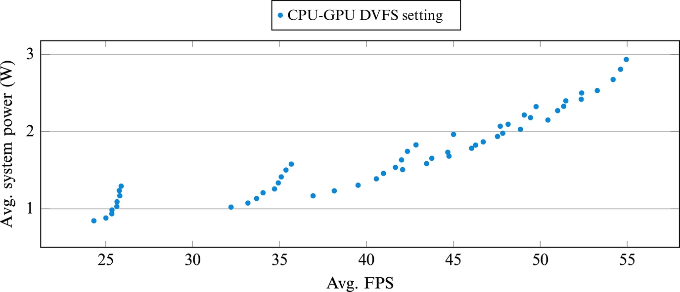
Exynos 5 Octa (5410) can perform CPU DVFS from 800 to 1600 MHz in nine discrete steps and GPU DVFS from 177 to 640 MHz in six discrete steps. In total, a game can be run on 54 static CPU-GPU DVFS settings. We run the Asphalt 7 racing game deterministically on each setting for 5 min and report the observed average FPS and power consumption in Fig. 6. The Asphalt 7 game loop runs at different speeds in different settings, resulting in a different average FPS for the game at each setting. Fig. 6 shows that a game can achieve the same level of FPS with different settings, whose power consumption can differ substantially. Fig. 6 also shows that reducing the FPS of a game can significantly reduce its power consumption. The challenge for a gaming governor is to choose the most power-efficient CPU-GPU DVFS setting for a given FPS among all settings. The most power-efficient setting will change over time as a game scene changes in complexity during the gameplay, but not substantially.
We chose FPS per unit CPU power and FPS per unit GPU power as a measure for CPU and GPU power-efficiency, respectively. Fig. 7A (or Fig. 7B) shows the power-efficiency of a CPU (or GPU) for the Asphalt 7 game when CPU (or GPU) frequency is increased, while keeping GPU (or CPU) at the highest frequency. Fig. 7 shows that the power-efficiency of both CPU and GPU decreases as their frequency is increased. We made a similar observation for almost all games. This observation greatly simplifies the power management algorithm for the gaming governor, since we know that if the desired FPS can be met by multiple different CPU (or GPU) frequencies, then the lowest among them will prove to be the most power-efficient.

2.4 Gaming Bottlenecks
Producer-consumer relationships between CPU and GPU in games as shown in Fig. 5 are subject to bottlenecks like any other producer-consumer relationship. If either CPU or GPU becomes a bottleneck, game performance cannot be increased irrespective of how fast the other component operates. The nonbottleneck component just ends up wasting power. In addition to resource bottlenecks, OS on HMPSoCs also limits the performance of the game to the refresh rate of the display (generally 60 Hz). If the game produces more than 60 FPS, then either CPU or GPU or both are operating faster than necessary, thereby wasting power. A game’s FPS can be directly measured from the OS kernel. For detecting resource bottlenecks, we found CPU and GPU utilizations as sufficient measures that are available on all platforms. We now show how these bottlenecks manifest themselves in real games.
Fig. 8 shows the effect of increasing GPU frequency for the CPU-bound game Edge of Tomorrow, when CPU is fixed at its highest frequency. Fig. 8A shows that FPS first increases with increase in GPU frequency, but then stops responding to GPU DVFS after 480 MHz and beyond. Fig. 8B shows that CPU utilization for the game reaches 100% at 480 MHz making CPU a bottleneck, and further performance gain from GPU DVFS beyond 480 MHz impossible. Fig. 9 similarly shows that saturation of GPU (100% utilization) is responsible for a GPU-bound game Bike Rider’s FPS to never respond to CPU DVFS. Finally, Fig. 10 shows the relatively simple FPS-bound game Deer Hunter whose FPS hits 60 FPS at the lowest CPU-GPU DVFS settings, leaving no further scope of increase in FPS with either CPU or GPU DVFS.


2.5 Performance Modeling
Based on Section 2.4, a game’s FPS will increase with increase in a component’s frequency (CPU or GPU) as long as it does not reach the upper limit of 60 FPS or the other component (GPU or CPU) becomes a bottleneck. We capture this behavior in the form of a linear mathematical model. All the constants in the model are determined using linear regression on data obtained from ten games.
Let FC and FG represent the current CPU and GPU frequency, respectively. ![]() ,
, ![]() , and
, and ![]() represent the FPS, CPU utilization, and GPU utilization at the CPU-GPU DVFS setting (FC, FG), respectively. We now attempt to estimate FPS at a higher frequency setting (FC′, FG′) from the current frequency setting (FC, FG). We assume a linear relationship between FPS and different CPU/GPU frequencies in the absence of a bottleneck. The relationship is captured using
represent the FPS, CPU utilization, and GPU utilization at the CPU-GPU DVFS setting (FC, FG), respectively. We now attempt to estimate FPS at a higher frequency setting (FC′, FG′) from the current frequency setting (FC, FG). We assume a linear relationship between FPS and different CPU/GPU frequencies in the absence of a bottleneck. The relationship is captured using
where γ1 and γ2 are constants obtained through linear regression.
Now we add the FPS bottleneck to the model. Let ![]() represent the maximum FPS a game can attain on the HMPSoC. Theoretically, it is the same as the display refresh rate (60 FPS) but some games also employ internal FPS control, which can limit a game’s FPS to a much lower value.
represent the maximum FPS a game can attain on the HMPSoC. Theoretically, it is the same as the display refresh rate (60 FPS) but some games also employ internal FPS control, which can limit a game’s FPS to a much lower value. ![]() for a game scene can be easily obtained by setting CPU and GPU together at their highest frequency, while the game scene is executing. The following equations model the FPS bottleneck.
for a game scene can be easily obtained by setting CPU and GPU together at their highest frequency, while the game scene is executing. The following equations model the FPS bottleneck.
Now we add the resource bottlenecks to the model. Let ![]() and
and ![]() represent the maximum CPU and GPU utilization for a game, respectively. Theoretically, maximum value of utilization is 100% but in practice the value can be much lower due to memory access latency or memory bandwidth saturation.
represent the maximum CPU and GPU utilization for a game, respectively. Theoretically, maximum value of utilization is 100% but in practice the value can be much lower due to memory access latency or memory bandwidth saturation. ![]() and
and ![]() can be obtained by sampling at the extreme CPU-GPU DVFS settings. We obtain
can be obtained by sampling at the extreme CPU-GPU DVFS settings. We obtain ![]() (or
(or ![]() ) for a game scene by setting CPU (or GPU) at the lowest frequency, while keeping GPU (or CPU) at the highest frequency. The following equations model the resource bottlenecks.
) for a game scene by setting CPU (or GPU) at the lowest frequency, while keeping GPU (or CPU) at the highest frequency. The following equations model the resource bottlenecks.


2.6 Utilization Models
We also need a utilization model to predict bottlenecks before they happen. When a component’s frequency is increased and the FPS remains unchanged, then the component’s utilization must decrease. This will be true only if the component is not itself a bottleneck and holding the FPS back. Utilization of a component will remain unchanged if it is the bottleneck because the component will be able to process more frames (and hence more utilization) with an increase in its clock frequency. This is captured mathematically by


where α1 and β1 are constants.
Utilization of a component (CPU or GPU) is also affected by a change in frequency of the other component (GPU or CPU) even if the frequency of the component of interest (CPU or GPU) is kept constant. This is because if the other component (GPU or CPU) frequency is increased, then the fixed frequency component (CPU or GPU) will have more work to do in the form of more frames to process at the same frequency. This behavior is captured by
where α2 and β2 are constants.
2.7 Gaming Governor
Based on our models presented in previous sections, we design a governor for mobile games. The goal of the gaming governor we design is to execute a game at a target FPS provided by the user with minimal power consumption. It was already shown in Section 2.3 that a game consumes less power at a lower FPS, but an acceptable level of FPS will differ from one user to another. For a professional gamer with eyes very attuned to a high refresh rate, anything less than 60 FPS will be unacceptable. On the other hand, for a casual gamer, 30 FPS will be sufficient. Therefore it is best for the user to provide the desired level of performance manually.
Further, it was also shown in Section 2.3 that the lowest power-consuming CPU-GPU DVFS setting for a given FPS is the setting in which CPU and GPU frequencies are the lowest possible under the FPS constraint. Thus the goal of our gaming governor is to find the lowest CPU-GPU DVFS setting where the user-defined FPS can be met. Our gaming governor operates at a granularity of 1 Hz.
When a game scene starts, we take three samples (each of duration 1 s) to obtain game-specific upper-bound constants ![]() ,
, ![]() , and
, and ![]() . Game scenes generally last a long time, and the benefits of taking these samples in the beginning far outweighs the momentary drop in user experience. These samples greatly enhance the accuracy of our models and also avoid any requirement of prior offline profiling.
. Game scenes generally last a long time, and the benefits of taking these samples in the beginning far outweighs the momentary drop in user experience. These samples greatly enhance the accuracy of our models and also avoid any requirement of prior offline profiling.
Initially in the models, we use coefficients that are obtained from our regression analysis. This provides a good estimate to set initial CPU-GPU frequencies for achieving the target FPS. As the game progresses, a sample is taken from the game every second. These samples from additional data to further refine our regression models online and tailor the models to the scene currently being rendered. This runtime regression has a very low overhead of approximately 0.08% on the CPU. The governor’s total overhead on the CPU is 2%, attributed mostly to the complex process of extracting FPS information from kernel log dumps.
Our governor can target any FPS, but to simplify the explanation, we assume the highest FPS ![]() as our target. At the present CPU-GPU DVFS setting (FC, FG), we can either be below the maximum FPS (
as our target. At the present CPU-GPU DVFS setting (FC, FG), we can either be below the maximum FPS (![]() ) or at it (
) or at it (![]() ).
).
Meeting FPS
If ![]() , then either CPU is the bottleneck (
, then either CPU is the bottleneck (![]() ) or GPU is the bottleneck (
) or GPU is the bottleneck (![]() ). We need to identify the bottleneck component and increase its frequency to increase FPS. Let us assume the required DVFS setting is (FC′, FG′), where FC′≥ FC and FG′≥ FG.
). We need to identify the bottleneck component and increase its frequency to increase FPS. Let us assume the required DVFS setting is (FC′, FG′), where FC′≥ FC and FG′≥ FG.
If CPU is the bottleneck, then we need to increase CPU frequency using the following equation derived from Eq. (3).

This increased CPU frequency should increase the FPS, but it may happen that we may still not see ![]() because bottlenecks switch, and GPU now becomes a bottleneck at its current frequency FG. GPU utilization at FC′ is given by the following equation derived from Eq. (10).
because bottlenecks switch, and GPU now becomes a bottleneck at its current frequency FG. GPU utilization at FC′ is given by the following equation derived from Eq. (10).
If ![]() , then GPU will become a bottleneck that has to be widened to realize FPS
, then GPU will become a bottleneck that has to be widened to realize FPS ![]() by increasing GPU frequency to FG′. FG′ is given by the following equation derived from Eq. (8).
by increasing GPU frequency to FG′. FG′ is given by the following equation derived from Eq. (8).

Similarly, if GPU were the bottleneck instead of CPU to begin with, then we would have evaluated FG′ first using Eq. (4). We would have checked for a possible CPU bottleneck using Eq. (9) and if required set it to a higher frequency FC′, based on Eq. (7).
Saving power
Now we focus on the other possibility where we are meeting the maximum FPS requirement on our current DVFS setting itself ![]() . This setting, though meeting our demand, may still be wasting power if CPU and/or GPU are not at their maximum utilization. If
. This setting, though meeting our demand, may still be wasting power if CPU and/or GPU are not at their maximum utilization. If ![]() , then we can save power by reducing CPU frequency to FC″ using the following equation derived from Eq. (7).
, then we can save power by reducing CPU frequency to FC″ using the following equation derived from Eq. (7).

Similarly, if ![]() , then we can save power by reducing the GPU frequency to FG″ using following equation derived from Eq. (8).
, then we can save power by reducing the GPU frequency to FG″ using following equation derived from Eq. (8).

2.8 Results
We use 20 games in our work. We divide them into two equal sets of 10 games each. We use the first set as the learning set to train our regression model. The second set is used as the testing set to evaluate the model in making predictions on unseen games. Tables 1 and 2 show the average error of our model in predicting performance at all DVFS setting for games in the learning and the test set, respectively. Average error in predicting FPS is only 3.87%.
Table 1
FPS Prediction Errors for Games in the Learning Set
| Edge of Tomorrow | Deer Hunter | Call of Duty | Jet Ski | Dhoom 3 | Bike Rider | D-Day | Turbo | MC3 | Godzilla |
| 2.39% | 0.08% | 2.11% | 3.63% | 3.48% | 11.41% | 3.32% | 13.91% | 11.41% | 1.30% |

Table 2
FPS Prediction Errors for Games in the Testing Set
| Farmville | Contract Killer | RoboCop | Dark Meadow | Revolt | AVP | Asphalt | I, Gladiator | Call of Dead | B&G |
| 0.26% | 0.21% | 5.23% | 5.48% | 4.58% | 0.02% | 0.09% | 7.64% | 4.90% | 1.02% |

We then test our approach against the default Linux Conservative governor [6] on a set of 10 games, chosen equally from the learning and the test set. The results are presented in Fig. 11. Linux always aims for the highest performance, so we also set maximum FPS as the target for our gaming governor. Both governors result in the same performance (≈ 60 FPS) for the games but consume different amounts of power. Therefore HMPSoC’s power-efficiency under the two approaches when measured as FPS per unit power is directly comparable. Evaluations show our proposed gaming governor can provide on average 29% additional power-efficiency.

3 GPU Power Management for GPGPU Applications
In the previous section, we discussed the state-of-the-art power management techniques to reduce power consumption of mobile games running on HMPSoCs. Recent advancements in the mobile GPUs have empowered the user to run not only games but also GPGPU applications. This section discusses the state-of-the-art techniques proposed for executing such applications on mobile GPUs.
3.1 State-of-the-Art Techniques
There has been tremendous interest in optimization techniques for performance and power-efficiency in heterogeneous platforms containing GPUs [14–17]. Conventionally, the multicore CPUs in these heterogeneous systems are used for general-purpose tasks, while the data-parallel tasks in the applications exploit the integrated or discrete GPU for accelerated execution [15]. However, most of the research in the past focused on PC-class CPU-GPU systems [14–18]. Unlike PC-class CPU-GPU systems, GPGPU applications executing on HMPSoCs also need to deal with the effects of resource sharing between CPU and GPU [19–21]. This necessitates appropriate consideration to coordinate both the CPU and the GPU so as to maximize performance. Wang et al. [19] took the total chip power budget of the AMD Trinity single-chip heterogeneous platform into consideration to propose a runtime algorithm that partitions the workload as well as the power budget between the CPU and the GPU to improve throughput. Wang et al. [21] also showed that in coordinated CPU-GPU runs on a similar AMD platform, there is a higher possibility of the CPU and the GPU accessing the same bank because of the similarity of memory access patterns, resulting in memory contention. Paul et al. [20] proposed techniques to address the issue of shared resources in integrated GPUs in AMD platforms. Additionally, DVFS techniques were used to achieve energy-efficient executions.
In the context of targeting GPGPU workloads toward mobile platforms, several early works [22–26] only explored image processing and computer vision applications on mobile GPUs [27]. Work presented in Refs. [22, 23] explored the implementation, optimization, and evaluation of image processing and computer vision applications, such as cartoon-style nonphotorealistic rendering, and stereo matching, on the PowerVR SGX530 and PowerVR SGX540 mobile GPUs. Ref. [24] executed a face recognition application on the Nvidia Tegra mobile GPU and achieved 4.25× speedup by using a CPU-GPU design rather than a CPU-only implementation. Ref. [25] presented the first implementation of local binary pattern feature extraction on a mobile GPU using a PowerVR SGX535 GPU. The authors concluded that, although GPU alone was not enough to achieve high performance, a combination of CPU and GPU improved performance as well as energy-efficiency. Work presented in Ref. [26] showcased an efficient implementation of the scale-invariant feature transform (SIFT) feature detection algorithm on several mobile platforms such as the Snapdragon S4 development kit, Nvidia Tegra 3-based Nexus 7 among others. The authors partitioned the SIFT application so as to execute different parts of the application in CPU and GPU in a producer-consumer fashion. They achieved considerable speedup for CPU-only optimized design, while also improving energy-efficiency.
While all of these early works focused only on image processing and related algorithms as GPGPU applications, the current mobile GPUs have advanced to the point of implementing a wide range of parallel applications [27]. Moreover, the growing popularity and support for OpenCL in mobile GPUs has also simplified GPU computing, thereby enabling several other types of GPGPU applications [27, 28].
Maghazeh et al. [28] explored GPGPU applications on a low power Vivante GC2000-embedded GPU on the i.MX6 Sabre Lite development board and compared it to a PC-class Nvidia Tesla GPU. Their platform supports OpenCL Embedded Profile 1.1, which implements a subset of the OpenCL Full Profile 1.1 APIs. The authors demonstrated that different applications behave differently on CPU and GPU and argued for the benefit of using CPU and GPU simultaneously for performance and energy-efficiency.
Grasso et al. [27] focused on examining the performance of the Mali GPU for high-performance computing workloads. They identified several OpenCL optimization techniques for both the host and the device kernel code so as to use the GPU more efficiently. In order to exploit the unified memory system in the HMPSoC, they optimized the memory allocations and mappings in the host code. They also proposed to manually tune the work-group size of the OpenCL kernels in order to maximize the resource utilization of the GPU, thereby achieving higher performance. Several other optimization techniques for the kernel code, such as vectorization based on the GPU architecture and thread divergence issue for GPUs, were also proposed in their work to improve performance of the GPU. This work mainly targeted the GPU, without considering the CPU to further improve performance.
Chandramohan et al. [29] presented a workload partitioning algorithm for HMPSoCs, while considering shared resources and synchronization. Their HMPSoC contained dual-core Cortex-A9 processor, dual-core Cortex M3 processor, and C64X+ digital signal processor (DSP). They tested several workload partitioning policies on these compute devices based on the individual throughput, frequency, and so on, and ultimately proposed an iterative partitioning technique based on load balancing to achieve high performance. However, they missed the opportunity to use the mobile GPU for executing any part of the workload. Furthermore, their iterative technique is shown to perform worse than the best possible results achievable on their platform, as found from exhaustive design space exploration.
Jo et al. [30] designed their OpenCL framework to support specifically ARM CPUs. A similar open-source framework, FreeOCL [31], was also developed for ARM CPUs to enable the CPU to act as the host processor as well as an OpenCL compute device. In an effort to improve cache utilization and load balancing, Seo et al. [32] proposed a technique to automatically select the optimum work-group size for OpenCL kernels on multicore CPUs. The ideas proposed in their work can also be used to improve performance in mobile GPUs.
Existing literature on exploiting mobile GPUs for general-purpose computing is quite sparse. They also do not consider the DVFS capabilities of the latest HMPSoCs in order to save power and energy. Moreover, with the increasing number of cores in the accompanying CPUs, it is equally important to exploit CPU and GPU concurrently for a single kernel in order to achieve increased performance as well as energy-efficiency. However, it is a nontrivial task to obtain optimal load partitioning of a single kernel on the CPU and GPU, especially while considering the effect of resource contention in a HMPSoC.
We now proceed to discuss techniques proposed in our recent work [33] to exploit the GPU along with the accompanying CPU in HMPSoCs to achieve high performance for diverse GPGPU kernels. Furthermore, we demonstrate a way to obtain the best DVFS settings for GPU and CPU in order to improve energy-efficiency.
3.2 Background
3.2.1 Hardware environment
While the gaming workloads were evaluated on the Odroid XU+E development platform, we explore the GPGPU applications on the Odroid XU3 [34] mobile application development platform as shown in Fig. 12. This platform features the Exynos 5 Octa (5422) HMPSoC comprising a quad-core Cortex- A15 CPU cluster, a quad-core Cortex- A7 CPU cluster, and a hexa-core (arranged in two clusters of 4-core and 2-core) Mali-T628 GPU. Unlike the Exynos 5 Octa (5410) HMPSoC in the Odroid XU+E platform, the Exynos 5 Octa (5422) HMPSoC allows all the eight CPU cores to function simultaneously. This feature is extremely important for GPGPU applications in order to employ all eight cores of the two CPU clusters for OpenCL execution, unlike only one CPU cluster being available at any given time in the Exynos 5 Octa (5410) HMPSoC. Furthermore, all eight cores of the CPU and four cores (only the four-core cluster of this GPU supports OpenCL) of the GPU support concurrent execution of OpenCL kernels.

Each of the CPU clusters, namely the A15 and A7, allows extensive DVFS settings for power and thermal management. The frequency of the A15 cluster, for example, can be set between 200 and 2000 MHz, while the A7 cluster can be clocked between 200 and 1400 MHz, both at an interval of 100 MHz. The accompanying Mali-T628 MP6 GPU on this platform is based on the ARM’s Midgard architecture and implements six shader cores that can execute both graphics and general-purpose computing workloads. However, the OpenCL runtime uses only four shader cores during OpenCL execution. The GPU L2 cache (128 KB) is shared between the shader cores. However, the GPU L2 cache is not kept coherent with the CPU L2 cache, even though the GPU is allowed to read from the CPU cache. The main component of the shader core is a programmable massively multithreaded tri-pipe processing engine. Each tri-pipe consists of a load-store pipeline, two arithmetic pipelines and one texture pipeline. The texture pipelines are not used during OpenCL execution. The arithmetic pipeline is a very long instruction word (VLIW) design with single-instruction multiple-data (SIMD) vector characteristics that operate on registers of 128-bit width. This means that the arithmetic pipeline contains a mixture of scalar and vector (SIMD) arithmetic logic units that can execute a single long instruction word. The load-store pipeline of each shader core has 16 KB L1 data cache. The tri-pipe is capable of concurrently executing hundreds of hardware threads. The memory latency of threads that are waiting on memory can be effectively hidden by executing other threads in the arithmetic pipeline. The ARMMidgard architecture used in this GPU differs significantly from other GPU architectures in the sense that the arithmetic pipelines are independent and can execute threads that are different, for example, in case of divergent branches and memory stalls. The available voltage-frequency settings for this GPU are shown in Table 3.

3.2.2 Software environment
In our work we heavily rely on OpenCL, a parallel programming language, to exploit the heterogeneity in our platform to achieve energy-efficiency. In this section, we briefly explain the OpenCL programming model followed by our technique of partitioning the application across the CPU and GPU cores.
OpenCL background
OpenCL is an open-source programming language for cross-platform parallel programming in modern heterogeneous platforms. It can be used develop applications that are portable across devices with varied architectures such as CPU, GPU, field-programmable gate array (FPGA), etc. Device vendors are responsible for providing OpenCL runtime as well as compilation tools to support OpenCL on their devices. Moreover, multiple OpenCL runtime software can coexist on a single platform, thereby allowing applications to concurrently exploit various devices in the platform.
The OpenCL programming model allows a host code segment that runs on the CPU to schedule the computations using the OpenCL kernels on one or more compute devices. A CPU, GPU, DSP, or even FPGA can act as a compute device. The initialization and setup of these compute devices is performed by the host code, which then uses OpenCL API functions to schedule kernels for execution. The host code is also responsible for transferring the data to and from the compute devices before and after the kernel execution, respectively. The kernel or device code is built on the host CPU with the help of OpenCL APIs during runtime before getting scheduled on the compute device for execution.
Each of the compute devices (e.g., GPU) consist of several compute units (e.g., shader cores in Mali), whereas the compute units consist of processing elements (e.g., arithmetic pipelines). A work-item refers to a kernel instance that operates on a single data point and is executed on a processing element. A work-group contains a group of work-items that are simultaneously executed on the processing elements of a single compute unit. The term NDRange refers to the index space of the input data for data-parallel applications. All work-items of an OpenCL program operate along this NDRange and execute identical codes. However, they may follow different control paths based on the input data instance on which they operate. The OpenCL execution model can be related to the popular Compute Unified Device Architecture (CUDA) model by visualizing the OpenCL work-item as a CUDA thread, work-group as a thread-block, and NDRange as the grid. The OpenCL work-items have a private memory, whereas every work-group has a local memory that is shared by all the work-items within the work-group. The work-groups also have access to a global memory that can also be accessed by the host. The memory model defined in OpenCL mandates memory consistency across work-items within a work-group; however, this is not required among various work-groups. This feature allows different work-groups to be scheduled on different compute devices (e.g., CPU and GPU) without a need to ensure memory consistency among the devices.
OpenCL runtime
ARM supplies the OpenCL runtime software for the Mali GPU to promote the usage of the GPU for GPGPU applications. On the other hand, current HMPSoCs typically do not ship with OpenCL support for their ARM CPUs [30]. Hence, in order to explore the concurrent execution of OpenCL applications on CPU alongside the GPU, we compile and install an open-source OpenCL runtime called FreeOCL [31] on our HMPSoC. This enables usage of all the eight CPU cores (four big and four small cores) as OpenCL compute units. From the perspective of the OpenCL programmer, there is no difference between the different core types. Moreover, unlike other open-source OpenCL runtimes such as [35], FreeOCL also enables us to launch an OpenCL kernel concurrently on all CPU cores and GPU.
OpenCL code partitioning across CPU-GPU
The pseudocode shown in Algorithm 1 describes the strategy used in partitioning an OpenCL application workload across the CPU and GPU cores. Given an application, the fraction of work-items to be executed on each device is obtained statically. During OpenCL execution, the workload (global_work_size) on both CPU and GPU needs to be a multiple of the work-group size (Line 1). Hence splittingPoint, which is used as the reference point for splitting, is obtained as the number of work-groups nearest to the desired fraction of the CPU workload (split_fraction). Subsequently, the global work-size and offset values for the CPU and GPU are obtained based on this splittingPoint as shown in the pseudocode (Lines 2–7). The partitioned workload is then executed by enqueuing kernels on both devices with the new global work-size and offset values (Lines 9–10).

3.3 GPGPU Applications on Mobile GPUs
The y-axis in Fig. 13 shows that the runtime execution for the OpenCL kernels from the PolyBench benchmark suite [36] on all CPU cores (4 A7 + 4 A15), GPU cores, and when optimally partitioned for performance across the CPU and GPU cores. Each cluster is set to run at its maximum frequency for this experiment. We reinforce additional environmental cooling to maintain the chip below its thermal design power in order to avoid thermal throttling. It can be seen from the figure that, while many applications run significantly faster on the GPU, others exhibit shorter runtimes on the CPU. However, most of the applications run significantly faster while running on both the CPU and the GPU. The percentage of runtime improvement for CPU + GPU execution over the best of the CPU-only and GPU-only executions is shown on the secondary y-axis. The improvement in runtime can be up to 40% and on average 19% across all the benchmarks. This experiment clearly establishes that even those GPGPU applications that run much faster when running only on the GPU than on the CPU, can also benefit significantly from concurrent CPU + GPU execution.

3.4 DVFS for Improving Power/Energy-Efficiency
While the concurrent execution helps in terms of performance as shown in the previous section, we also need to explore the various DVFS settings in order to achieve high power/energy-efficiency. Fig. 14 illustrates the energy-performance trade-off for 2DCONV and SYR2K applications from the PolyBench suite, while executing on CPU alone, GPU alone, and when optimally partitioned between CPU and GPU, with various DVFS settings of the CPU and GPU. The y-axis shows the energy consumption in Joules, while the x-axis plots the execution time in seconds in log scale. Table 4 shows the DVFS settings used for these experiments.

Table 4
DVFS Settings for Design Space Exploration
| Test | A7 Frequency | A15 Frequency | GPU Frequency |
| Configuration | (MHz) | (MHz) | (MHz) |
| CPU-only (A7 +A15) | 1400 | 1000–2000 | Not applicable |
| GPU-only | Not applicable | Not applicable | 177–600 |
| CPU + GPU (A7 +A15 + GPU) | 1400 | 1000–2000 | 177–600 |

It can be observed from Fig. 14 that different applications behave very differently based on their individual characteristics. The 2DCONV application benefits significantly from the GPU (GPU-bound), and therefore the GPU-only execution points are close to the Pareto-front with very low-energy consumption, whereas the CPU-only design points are much farther away. On the other hand, the SYR2K application is heavily reliant on the CPU (CPU-bound), and therefore the CPU-only (A7 +A15) execution points are closer to the Pareto-front with higher performance (low execution time) than the GPU-only designs.
In addition, it can also be seen that energy-efficiency can be improved by running at lower DVFS settings (black circles), when compared to the highest frequency settings (black boxes), without significant degradation in the performance of the execution time. The design space for the 2DCONV and SYR2K applications as shown in Fig. 14, include the optimal ED2 point, highlighted as a black circle on the Pareto-front. The CPU-GPU (A7, A15—GPU) frequency (in MHz) combination, and the CPU workload fraction (in %) for the optimal ED2 point for 2DCONV and SYR2K applications are (1400, 1000–600, 21%) and (1400, 1600–600, 71%), respectively. Power consumption is also reduced significantly at these points (black circles) since the energy reduces significantly, while the execution time increases by only a small margin. However, due to the large number of possible DVFS settings as well as the application partitioning between CPU and GPU, it is a challenging task to choose the optimal design point.
In the next section, we introduce the proposed static partitioning plus frequency selection technique to generate the Pareto-optimal design points. In order to simplify the quantitative evaluation of the proposed solution, we use the ED2 metric (energy × delay × delay) that encapsulates the energy-performance trade-off. This metric gives additional weightage to the delay term to ensure that we choose points with the least degradation in the execution time performance, while achieving the largest possible power/energy savings.
3.5 Design Space Exploration
In the previous section, it was shown that the concurrent execution of an optimally partitioned application between CPU and GPU not only helps in reducing the execution time but also the energy with appropriate DVFS settings. This section discusses the proposed techniques to obtain the appropriate workload partitions and DVFS settings for the optimal ED2 value.
3.5.1 Work-group size manipulation
As discussed earlier in Section 3.2, each kernel instance in OpenCL is a work-item, while a group of work-items constitute a work-group. Prior to partitioning the work-groups between the CPU and GPU cores, an appropriate work-group size must be selected in the first step. Seo et al. [32] discussed the various challenges as well as the benefits of selecting the optimum work-group size for OpenCL applications executing on the CPU, especially to improve cache utilization. Similar challenges and benefits also apply to executing OpenCL applications on the GPU, and even more so in case of mobile GPUs because of the limited amount of cache available in these devices. We observe that the work-group size does not impact the CPU performance on our platform because of sufficient cache capacity, but it significantly affects the GPU performance. Therefore we find the optimal work-group size for the GPU and use the same value of the work-group size for both CPU and GPU.
The maximum work-group size that can be selected for Mali GPU is 256 [37]. However, this maximum size cannot be guaranteed for all applications. OpenCL provides API to obtain the maximum possible work-group size for a given kernel, but this may not necessarily be the optimal work-group size. The OpenCL runtime can also be employed to automatically select a work-group size for the kernel if there is no data sharing among work-items [37]. This does not always produce the best results [27].
In order to obtain the best work-group size for an application, we employ a simple technique. It is noteworthy that the value of the work-group size is preferred to be in powers of two [37]. Hence we exhaustively explore all work-group size in powers of two up to the maximum possible work-group size for the given application and select the one that provides the best performance. Fig. 15 shows the improvement in execution time with selected work-group size compared to the default work-group size as originally specified in the PolyBench suite. Some applications such as 2DCONV and 3DCONV show minimum or no improvement in performance as the default work-group size is itself the optimal value. Overall, using the best work-group size can lead to an average of 40% performance improvement. We perform the subsequent partitioning and frequency selection for applications with this best work-group size.

3.5.2 Execution time and power estimation
In order to select the appropriate DVFS point for the GPU and CPU clusters, we first model the impact of frequency scaling on the power-performance behavior of an OpenCL kernel. After estimating the behavior of GPU and CPU independently, we subsequently include the impact of memory contention between the two.
GPU estimation
In order to estimate the power-performance of a given application on the GPU, we first sample its runtime and power at the minimum (177 MHz) and maximum (600 MHz) GPU frequencies. We then predict the performance and power for the remaining frequency points. During the execution of OpenCL kernels on the GPU, the utilization always stays at 100%. Hence the runtime can be safely modeled using a linear relationship, as shown in Eq. (16).
Here T is the execution time, f is the frequency, and α, β are constants obtained through interpolation from the runtime at two extreme points.
The total power (Ptotal) of the GPU core is estimated using Eq. (17), where A is the activity factor, C is the capacitance, V is voltage, f is frequency, and Pi is the idle power at the corresponding frequency setting.
In the first term, since we have a constant activity of 100% for our workload, we group C and A together and regard them as one constant c. This constant term is determined by taking the average of the values calculated from the experiments at the two extreme frequency settings. The idle power Pi is obtained through experiments performed once at each frequency setting.
In order to compute the estimation error, we also execute the applications at all the GPU frequency points and record the actual runtime along with power consumptions. Fig. 16 shows the estimation error in runtime and power estimation for GPU-only execution. Fig. 16 confirms the applicability of the linear model, which results in a low average estimation error of ≈ 0.5% in runtime and ≈ 1% in power consumption.

CPU estimation
Similar to the estimation for the execution time and power consumption during GPU-only execution, we also obtain the model for CPU-only execution. In order to estimate the effect of DVFS, we sample the execution time and power consumption of the OpenCL kernel at the minimum (200 MHz for A15, 200 MHz for A7) and maximum (2000 MHz for A15, 1400 MHz for A7) frequencies for each cluster. We then predict the performance and power for the remaining frequency points. During the OpenCL kernel execution, all the CPU cores are utilized to the maximum 100% as the FreeOCL runtime schedules multiple work-groups to a single CPU core similar to Ref. [30]. Therefore similar to the GPU-only execution, we use the linear model in Eq. (16) to estimate the execution time and Eq. (17) for power consumption at the other CPU frequency settings between the two extremes.
In order to evaluate the accuracy of the proposed technique, we also run the kernel at all possible frequency values to obtain the actual runtime and power consumption for each application. Fig. 17A and B shows this average error in execution time and power estimation for A15 and A7 clusters, respectively. The linear model serves well in this case and leads to an average estimation error of less than 2% in execution time and less than 6% in power consumption.

Concurrent execution and effect of memory contention
While running the application kernels concurrently on CPU and GPU cores, let us assume that we select a fraction N of the work-items to run on the CPU cores, while the rest run on the GPU at a particular DVFS setting. Now, we need to estimate the execution time and power for concurrent execution. Eq. (18) estimates the runtime for the entire application after partitioning between CPU and GPU, where TCPU and TGPU are the estimated runtimes for CPU-only and GPU-only execution at the DVFS setting, respectively.
In order to estimate the total power consumption in this case, we add the estimated power consumption of individual devices at the DVFS setting.
In Fig. 18, the first columns show the estimation error in runtime for concurrent execution, averaged across various DVFS settings. In this case, we identify the best partitioning point for each DVFS setting (the method to derive this is discussed next), observe the power and runtime for concurrent executions and compute the error compared to values obtained from actually running the application on our platform at similar settings. It can be observed from the figure that, while the average error remains less than 10%, few applications incur relatively large estimation error. This can be attributed to the contention for memory bandwidth between the CPU and GPU, especially in applications that demand larger memory bandwidth. Hence the effect of memory contention must be accounted for while estimating the execution time for concurrent execution.

We model the impact of this contention by obtaining the reduction in the instructions per cycle (IPC) value of a compute device when executing concurrently with another compute device. We first set the GPU at the lowest (177 MHz) and highest (600 MHz) frequencies, while keeping the CPU idle and running the GPU-only portion of the partitioned workload. Next, we again set the GPU at the two extreme frequencies, but this time the CPU runs in parallel with its portion of the partitioned workload. Fig. 19 shows the reduction in the IPC of the GPU because of the sharing of memory bandwidth with the CPU during concurrent execution when compared to the GPU-only execution at the highest GPU frequency. Similar results are also observed at the lowest GPU frequency setting. We used this reduction in IPC at the two extreme GPU frequencies in a linear model to account for the memory contention at other GPU frequencies. This contention effect (reduction in IPC) is then considered while estimating concurrent execution time in order to reduce the estimation error. The second column in Fig. 18 shows the estimation error in execution time averaged across various DVFS settings after incorporating this factor. It can be clearly seen that not only does the average estimation error drop from 7.6% to 4.8%, but also there is a significant reduction in the maximum error. Fig. 20 plots the power estimation error averaged across all DVFS points. It can be seen that the power estimation results are also quite accurate with an average estimation error of 5.1%.


CPU-GPU partitioning ratio
Now we focus on judiciously partitioning the kernels of an OpenCL application between the CPU and GPU based on their individual capabilities. We use a load balancing strategy for each application based on its runtime for CPU-only and GPU-only executions. In essence, this strategy splits the workload between CPU and GPU such that both compute devices take the same amount of time to finish executing their assigned workload portion. We partition the input data (global_work_size) of the OpenCL kernels for CPU and GPU before launching them concurrently on the two compute devices. Eq. (19) can be used to obtain the fraction (split_fraction) of the global_work_size of the application that should be executed on the CPU for the optimal load balancing.
Here m is the ratio of the execution time between CPU-only and GPU-only executions. We name the partitioning point as the “splittingPoint” to denote the splitting of the original global_work_size into two, one each for CPU and GPU.
In order to identify the best partitioning point as well as the DVFS settings, we first estimate the CPU-only, GPU-only performance and the power at each frequency setting using Eqs. (16), (17). Next, these individual power-performance estimations are used to obtain the best splittingPoint at each frequency setting with Eq. (19). We then estimate the runtime and power for concurrent execution with the selected splittingPoint. This gives us the runtime, power, as well as the energy consumption for every point in our design space shown in Fig. 14 and hence the Pareto-front.
In an effort to evaluate the power-performance improvement because of the proposed approach of employing both GPU and CPU cores, we select the point with the best energy-delay-squared product (ED2) from the design space. As discussed earlier in Section 3.4, the ED2 metric gives more weight to the execution time, which ensures minimal execution time degradation while still providing significant power and energy savings. Table 5 shows the DVFS settings (A15 CPU and GPU) and CPU workload fraction for the best ED2 design points. The frequency of the A7 CPU is set at 1400 MHz; however, this is not shown in the table to maintain clarity. Lastly, Fig. 21 shows the respective performance degradation and power savings at optimal ED2 point (similar to black circles in Fig. 14 for 2DCONV and SYR2K applications) compared to maximum frequency settings (similar to black boxes in Fig. 14 for 2DCONV and SYR2K applications). Most applications exhibit significant power savings with negligible degradation in execution time (less than 10%).

Table 5
Frequency Setting and CPU Workload Fraction for Optimal ED2
| App. Name | Frequency (MHz) | CPU Workload Fraction | App. Name | Frequency (MHz) | CPU Workload Fraction | ||
| CPU | GPU | CPU | GPU | ||||
| 2DCONV | 1000 | 600 | 0.21 | COVAR | 1800 | 600 | 0.52 |
| 2MM | 1600 | 600 | 0.37 | GEMM | 1000 | 600 | 0.12 |
| 3DCONV | 1400 | 600 | 0.29 | GESUM | 1600 | 600 | 0.77 |
| 3MM | 1400 | 600 | 0.28 | MVT | 1000 | 600 | 0.30 |
| ATAX | 1200 | 600 | 0.20 | SYR2K | 1600 | 600 | 0.71 |
| BICG | 1000 | 600 | 0.22 | SYRK | 1600 | 600 | 0.70 |
| CORR | 1800 | 600 | 0.52 | ||||

4 Future Outlook
We now discuss some problems we believe are still open in power management for mobile GPUs when running gaming or GPGPU applications.
4.1 Open Problems for Gaming Applications
In this chapter, we presented a gaming governor that operates efficiently by virtue of being sensitive to the complex relationship that mobile CPUs and GPUs exhibit when running mobile games. Still, many questions remain unanswered.
Ideal granularity at which a gaming governor should operate is yet to be found. The gaming governor we presented operated at a granularity of 1 s. In another approach, the gaming governor operates at a granularity of 50 ms [11]. The finer granularity a gaming governor operates at, the more variation in gaming workload it can exploit; but at the same time there is a power cost involved in doing DVFS. It is not clear which approach is better because a direct comparison between the two approaches with same games and same platform is yet to be made.
Research in gaming is held up by the unavailability of sufficient tools. There is no open-source GPU simulator that supports OpenGL; as a result, the impact of change in GPU architecture on power and performance of mobile games cannot be studied. There is also no standardized set of games that forms a comprehensive benchmark suite, where superiority of a gaming governor over other governors can be clearly established. Furthermore, there is no open-source OpenGL game that can match the sophistication of popular closed source games that are now ubiquitous on mobile platforms. This severely limits the ability of researchers to study the impact of source code and openGL compiler optimizations on a mobile game’s power-efficiency.
Some tools are available, such as Reran [38] and MonkeyGamer [39], that can replay a deterministic game, but no tool allows automatic gameplay that can simulate a real user for a nondeterministic game. Finally, every time a deterministic game runs, it produces similar but not exact workloads that are observed in previous runs. There are no tools available that can capture a gaming workload and allow its exact reproduction.
Thermal management of mobile platforms [40] is an active subject of research but is yet to be studied for mobile games. Power-efficient gaming governors would not necessarily also be thermally efficient. Memory management for mobile games also needs to be studied in detail, and it still remains to be seen what role the shared memory bus plays during mobile execution. Games are also perfect applications on which approximate computing can be applied to reduce power consumption.
Ref. [41] reduces CPU power consumption of mobile games on an asymmetric multicore CPU such as the one in Exynos 5 Octa (5422) HMPSoC, though not in conjunction with the GPU. We also observe that though CPU-bound games exist, most games are constrained by GPU rather than CPU. We already know that a CPU is capable of performing GPU workloads, so a GPU workload division can be explored similar to the workload partitioning performed in GPGPU applications.
4.2 Open Problems for GPGPU Applications
In this chapter, we discussed the identification of energy-efficient design points for GPGPU applications targeting mobile GPUs. However, we also observed that at higher frequencies (close to the maximum frequency), the HMPSoC quickly exhausts its thermal headroom and begins to throttle the CPU and GPU. This leads to a less than expected performance and also raises reliability concerns. In our current setup, we reinforced our HMPSoC with additional cooling measures to avoid such a scenario. In the future, the thermal budget can be taken into account while selecting the DVFS settings in order to proactively avoid hitting the thermal wall [42].
In addition, more complex applications, such as image processing and speech recognition, with multiple kernels can also be targeted toward mobile GPUs. However, as discussed in the Section 3, the accompanying CPU cores in the HMPSoC will also play an important role in these applications in order to achieve both performance and energy-efficiency. The workload partitioning between the GPU and CPU cores is a nontrivial task in the face of different power-performance trade-offs, multiple DVFS settings, and dynamic core scaling possibilities in such platforms.
The shared memory bandwidth between the CPU and GPU in a HMPSoC also poses additional challenges, as discussed earlier. The static solution proposed in this work might not provide optimal results in mobile phones when multiple applications are launched randomly to run on the CPU or GPU. Hence a runtime technique is necessary in such cases to monitor the memory traffic and perform appropriate DVFS of CPU and/or GPU to mitigate this effect.
The latest HMPSoCs discussed in this chapter contain performance heterogeneous ARM big.Little CPUs. The OpenCL runtime, however, treats them as similar processing elements and schedules the threads evenly across all CPU cores. In the future, the OpenCL runtime can be improved to take into account the performance heterogeneity of the processors, while also considering the CPU-GPU functional heterogeneity.
5 Conclusions
In this chapter, we first described the current state-of-the-art techniques for power management in mobile devices for both games and GPGPU applications. After identifying the limitations of the existing work, we discussed our latest power management techniques for these applications.
For games, a gaming-specific governor was presented that detects bottlenecks in CPU and GPU, and then accordingly increases the frequency of the bottlenecked component just enough to meet the game’s FPS target. The proposed governor reduced a HMPSoC’s power on average by 29% in comparison to the on-board stock Linux governor.
Next, we presented a static approach to save power and energy for GPGPU applications running on HMPSoCs. We considered the effect of contention because of the shared memory resources in a HMPSoC. Along with the appropriate partitioning of the OpenCL kernels to run on both CPU and GPU concurrently, suitable CPU-GPU DVFS settings were identified to save power and energy without a significant loss in performance. The approach saved more than 39% of power with minimal loss in performance when compared to the execution of GPGPU applications at the highest CPU-GPU DVFS setting.
Finally, we also identified possible future directions for research on reducing the power consumption of mobile GPUs while executing games or GPGPU applications. The rapid growth in the capabilities of the mobile GPUs as well as the other processing elements on HMPSoCs will continue to demand more sophisticated power management techniques.