
Accelerating GPU accelerators through neural algorithmic transformation
A. Yazdanbakhsh1; J. Park1; H. Sharma1; P. Lotfi-Kamran2; H. Esmaeilzadeh1 1 Georgia Institute of Technology, Atlanta, GA, United States
2 Institute for Research in Fundamental Sciences (IPM), Tehran, Iran
Abstract
Graphics processing units (GPUs) are many-core architectures that provide high performance by exploiting large degrees of data-level parallelism and employing the single instruction, multiple threads (SIMT) execution model. GPU can accelerate diverse classes of applications, including recognition, gaming, data analytics, weather prediction, and multimedia. Many of these applications are amenable to approximate execution. This application characteristic provides an opportunity to improve GPU performance and energy efficiency. Among approximation techniques, neural accelerators have been shown to provide significant performance and efficiency gains. This chapter describes our neurally accelerated GPU architecture that harmoniously embeds neural acceleration within GPU accelerators without hindering their SIMT execution while keeping hardware changes minimal.
Keywords
Throughput processor; Data-level parallelism; SIMT; Approximate computing; Acceleration; Neural network
1 Introduction
Historically, the improvement in processor performance was driven by two phenomena: Moore’s law [1] and Dennard scaling [2]. Technology scaling, which refers to the technology of shrinking transistor dimensions, provided processor designers with transistor density that doubled every 2 years (Moore’s law). Moreover, the reduction in the supply voltage enabled processor designers to operate twice the number of transistors that technology offers, without an increase in power consumption (Dennard scaling). Taking advantage of Moore’s law and Dennard scaling, computer architects improved the processing power by constantly increasing the complexity and frequency of processors. Decades of technology scaling allowed powerful processors with deep and aggressive Out-of-Order pipelines and high clock frequency to emerge.
Unfortunately, improving the performance of processors with the historical approach is no longer viable. As physical restrictions slow down the reduction of the supply voltage, Dennard scaling has effectively stopped [3]. While Moore’s law is still valid and the number of transistors increases by a factor of 2 every 2 years, the failure of Dennard scaling makes power and energy the primary constraints of processors. As such, it is no longer desirable to increase the clock frequency of processors or increase the complexity of the processor pipeline to improve performance, as these approaches are not energy efficient [4].
The diminishing returns from technology scaling [5–7] have coincided with an overwhelming increase in the rate of data generation. Expert analyses showed that in 2011, the amount of generated data surpassed 1.8 trillion GB, and the estimates indicate that consumers will generate 50× this staggering figure in 2020 [8]. On one hand, processing the ever-growing amount of generated data requires significant and continual boost of processors’ performance. On the other hand, we have reached the limits of an historical style of improving performance.
To overcome these challenges, both the semiconductor industry and the research community are exploring new avenues in computer architecture design. Two of the promising approaches are acceleration and approximation. Among programmable accelerators, graphics processing units (GPUs) offer significant performance and energy efficiency gains. While GPUs were originally designed to accelerate graphics functions, now they are being used to execute a wide range of applications, including recognition, learning, gaming, data analytics, weather prediction, molecular dynamics, multimedia, scientific computing, and much more. The availability of programming models for GPUs and the advances in their microarchitecture have played a significant role in their widespread adoption. Many companies, such as Microsoft, Google, and Amazon, use GPUs to accelerate their enterprise services. As GPUs play a major role in accelerating many classes of data-intensive applications, improving GPUs performance and energy efficiency is imperative to cope with the ever-increasing rate of data generation.
Many of the applications that execute on GPUs are amenable to imprecise execution [9–12]. This means that some variation in output of these applications is acceptable and some degradation in the output quality is tolerable. This characteristic of many GPU applications provides a unique opportunity to devise approximation techniques that trade small losses in the quality of the results for significant gains in performance and energy efficiency.
Many approximation techniques target approximable code. Approximable code is a segment of code that if approximated will not lead to catastrophic failures in execution (e.g., segmentation fault), and its approximation may lead only to graceful degradation of an application’s output quality. Among approximation techniques that target approximable code, neural acceleration, which provided significant gains for CPUs [13–17] is a good candidate for GPUs [18, 19]. Neural acceleration relies on an automated algorithmic transformation that converts an approximable segment of code to a neural network. A neural network is a family of models inspired by the brain and is used to approximate functions. There are algorithms to determine a good neural network for approximation of a given function. The transformation of a segment of code to a neural network is called the neural transformation [13]. The compiler automatically performs the neural transformation and replaces the approximable segment with an invocation of a neural hardware that mimics the behavior of that segment of code.
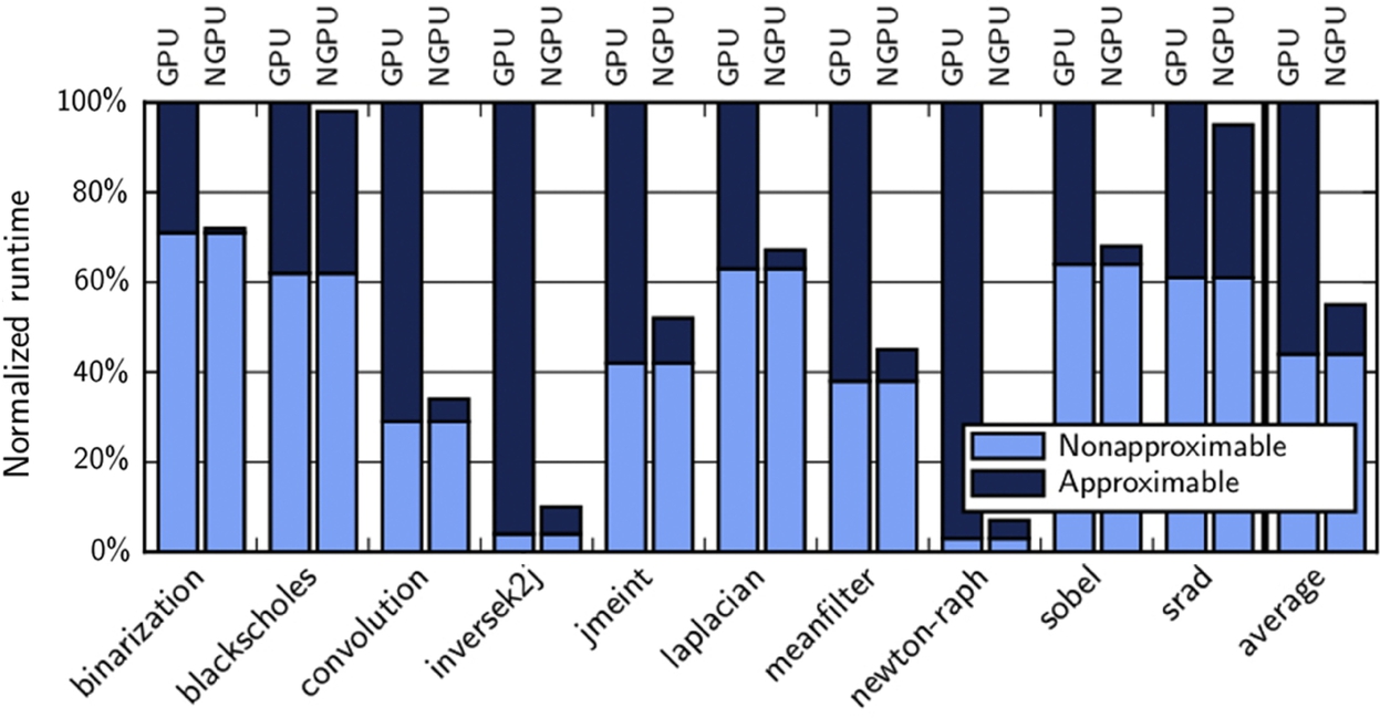
To demonstrate the potential benefits of neural acceleration in GPUs, we first study its applicability using a diverse set of representative GPU applications. Fig. 1 shows the breakdown of application runtime and energy dissipation between neurally approximable regions and the regions that cannot be neurally approximated. (The details of the breakdown methodology is discussed in Section 2. Section 6.1 presents our experimental methodology.) The neurally approximable segments are the ones that can be approximated by a neural network. Applications spend 56% of their runtime and 59% of their energy in neurally approximable regions on average. Some applications such as inversek2j and newton-raph spend more than 93% of their runtime and energy in neurally approximable regions. These results demonstrate that a significant fraction of time and energy of these GPU applications are spent on regions where neural accelerators can be applied to. Consequently, there is a significant potential for using neural acceleration on GPU processors.

Why hardware acceleration?
As previous work [20] suggested, it may be desirable to apply neural transformation with no hardware modifications and replace the approximable region with an efficient software implementation of the neural network that mimics the region. We explored this possibility and the results are shown in Fig. 2. On average, the applications suffer from 3.2× slowdown. Only inversek2j and newton-raph, which spend more than 93% of their execution time on the neurally approximable region, see 3.6× and 1.6× speedup, respectively. The slowdown with software implementation of neural network is due to (1) the overhead of fetching/decoding the instructions, (2) the cost of frequent accesses to the memory/register file, and (3) the overhead of executing the sigmoid function. The significant potential of neural transformation (Fig. 1) and the slowdown of the software-only approach (Fig. 2) necessities having GPU architectures with integrated hardware neural accelerators.

Why not reuse CPU neural accelerators?
Previous work [13] proposes an efficient hardware neural accelerator for CPUs. One possibility is to use CPU neural processing unit (NPU) for GPUs. However, as compared to CPUs, GPUs contain (1) significantly larger number of cores (single instruction multiple data [SIMD] lanes) that are also (2) simpler. Augmenting each core with an NPU that harbors several parallel processing engines and buffers imposes significant area overhead. Area overhead of integrating NPUs to a GPU while reusing SIMD lanes’ multiply-add units is 31.2%. Moreover, neural networks are structurally parallel. As such, replacing a code segment with neural networks adds structured parallelism to the thread. In the CPU case, NPU’s multiple multiply-add units exploit this added parallelism to reduce the thread execution time. GPUs, on the other hand, already exploit data-level parallelism and leverage many-thread execution to hide thread execution time. It has been shown that the added parallelism is not the main source of benefits from neural acceleration in GPUs [18, 19]. Consequently, neural acceleration in GPUs leads to a significantly different hardware design as compared to that of CPUs.
In the rest of this chapter, we first introduce the programming interface, compilation workflow, and ISA extension for the support of neural acceleration in GPUs. Then we explain the hardware extensions and modifications necessary to enable neural execution of threads in GPUs. Finally, we present the evaluation results of a GPU equipped with hardware neural accelerators and conclude.
2 Neural transformation for GPUs
To take advantage of hardware neural acceleration on GPUs, the first step is to have a compilation workflow that can automatically perform neural algorithmic transformation on the code. Moreover, there is a need for a programming interface that empowers code developers to delineate approximable regions as candidates for neural transformation. The section describes both the programming interface and the automated compilation workflow for GPU applications.
2.1 Safe Programming Interface
Any practical and useful approximation technique should guarantee execution safety. The safety guarantees prevent catastrophic failures such as out-of-bound memory accesses from happening due to approximation. In other words, approximation should never affect critical data and operations. The criticality of data and operations is a semantic property of a program and can be identified only by programmers. Therefore a programming language for approximate computation must offer ways for programmers to specify where approximation is safe. This requirement is commensurate with prior work on safe approximate programming languages, such as EnerJ [21], Rely [22], FlexJava [23], and Axilog [24]. For this goal, we extend the Compute Unified Device Architecture (CUDA) programming language with a pair of #pragma annotations that enable marking the beginning and the end of a safe-to-approximate region of a GPU application. The following example illustrates these annotations.
#pragma(begin_approx , “min max”)
mi = __min(r, __min(g, b));
ma = __max(r, __max(g, b));
result = ((ma + mi) > 127 * 2) ? 255 : 0;
#pragma(end_approx “min max”)
The preceding segment of code is approximable and is marked as a candidate for neural transformation by a programmer. The #pragma(begin_approx, “min_max”) indicates the segment’s beginning and associates a name (“min_max”) to it. The #pragma(end_approx, “min_max”) indicates the end of a segment that was named “min_max.”
It is worth mentioning that, in addition to what is presented in this section, there are other approaches for safe programming interfaces, such as EnerJ [21] that require annotating approximate data declarations. We chose to use #pragma to identify a segment of approximable code due to the lower annotation overhead, simplicity, and compatibility with the current CUDA compilers. However, the workflow presented in this chapter can also leverage other models if they are extended to CUDA.
2.2 Compilation Workflow
As discussed, the main idea of neural algorithmic transformation is to learn the behavior of a code segment using a neural network and then to replace the segment with an invocation of an efficient neural hardware [13, 18, 19]. To have this algorithmic transformation, the compiler needs to (1) identify the inputs and outputs of the segment of code; (2) collect the training data by observing (logging) the inputs and outputs; (3) find and train a neural network that mimics and approximates the observed behavior; and finally (4) replace that segment of code with instructions that configure and control the neural hardware. These steps are shown in Fig. 3. The compilation workflow is similar to the one described in Ref. [13] that targets CPU acceleration. However, the four steps have been specialized for GPU applications. Moreover, step (1) is done automatically to further automate the transformation.

1. Input/output identification. To find and train a neural network that mimics a code segment, the compiler needs to collect the input-output pairs that represent the functionality of the code segment. To this end, a compiler first needs to identify the inputs and outputs of the delineated segment. The compiler uses a combination of live variable analysis and Mod/Ref analysis [25] to automatically identify the inputs and outputs of the annotated segment. The inputs are the intersection of live variables in the beginning of the code segment and the set of variables that are referenced within the segment. The outputs are the intersection of live variables at the end of the code segment and the set of variables that are modified within the segment. In the previous example, this analysis identifies r, g, and b as the inputs to the segment and result as the output.
2. Code observation. After identifying the inputs and outputs of the segment, the compiler instructs these inputs and outputs to log their values in a file as the program runs. The compiler then runs the program with a series of representative input data sets (such as the ones from a program test suite) and logs the pairs of input-output values. The collected set of input-output values constitutes the training data that captures the behavior of the segment. The training data will be used in the next step to find and train a neural network for the code segment.
3. Topology selection and training. In this step, the compiler needs to both find a topology for the neural network and train it. While searching for a topology for the neural network, the objective is to strike a balance between the network’s accuracy and its overhead. Theoretically, a larger, more complex network offers higher accuracy potentials but is likely to be slower and less energy efficient than a smaller network. The accuracy of neural networks does not improve beyond a certain point even if they are enlarged. To pick a good topology, the compiler considers a search space for the neural topology and selects the smallest network that offers comparable accuracy to the largest network in the space. The neural network of choice in this study is multilayer perceptron (MLP) that consists of a fully connected set of neurons organized into layers: the input layer, any number of hidden layers, and the output layer. The number of neurons in the input and output layers is fixed and corresponds to the number of inputs and outputs to the code segment. The goal is to find the number of hidden layers and the number of neurons in each hidden layer.
As the space of all possible topologies is infinitely large we restrict the search space to neural networks with at most two hidden layers. The number of neurons per hidden layer is also restricted to the powers of 2, up to 32 neurons. These choices limit the search space to 30 possible topologies. The maximum number of hidden layers and the maximum number of neurons per hidden layer are compilation options and can be changed. All possible neural networks are trained independently in parallel. To pick the best fitting neural network topology, the input-output pairs obtained in step (2) are partitioned into a training data set (usually two-thirds of the pairs) and a selection data set (the remaining pairs). The training data sets are used to train a neural network (i.e., determine the weights of the connections) for a given topology, and the selection data sets are used to select the final neural network topology based on the observed application quality loss (the smallest topology that offers the lowest quality loss will be selected). Note that we use completely separate data sets to measure the final quality loss in Section 6.
For training the neural network using the training data sets, we use the standard backpropagation [26] algorithm. Our compiler performs 10-fold cross-validation for training each neural network. The output from this phase consists of a neural network topology—specifying the number of layers and the number of neurons in each layer—along with the weight of each connection that are determined by the training algorithm.
4. Code generation. After identifying the best neural network and having the weights for the connections, the compiler replaces the code segment with special instructions that send the inputs to the neural accelerator (we will talk about the details of the neural accelerator later in this chapter) and retrieve the results. The compiler also generates the configuration of the neural accelerator. The configuration includes the weights and the schedule of the operations within the accelerator. The configuration of the neural network is loaded into the integrated neural accelerators at the beginning when the program is loaded for the execution.
3 Instruction-set-architecture design
To enable neural acceleration, the instruction-set architecture of a GPU should have three instructions: (1) an instruction for sending the inputs to the neural accelerator; (2) an instruction for receiving outputs from the neural accelerator; and finally (3) an instruction for sending the accelerator configuration and the weights. For this purpose, we extend the Parallel Thread Execution (PTX) ISA, which is used in Nvidia’s CUDA programming environment with the following three instructions:
1. send.n_data %r. This instruction sends the value of register %r to the neural accelerator. The instruction also informs the accelerator that the value is an input and not a configuration.
2. recv.n_data %r. This instruction retrieves a value from the accelerator and writes it to the register %r.
3. send.n_cfg %r. This instruction sends the value of register %r to the accelerator. The instruction also informs the accelerator that the value is for setting the configuration of the neural accelerator.
We use PTX ISA version 4.2. PTX 4.2 supports vector instructions that can read or write two or four registers. We take advantage of this feature and introduce two vector versions for each of our instructions. The send.n_data.v2 {%r0, %r1} sends two register values to the accelerator and a single send.n_data.v4 {%r0, %r1, %r2, %r3} sends the value of four registers to the neural accelerator. The latter instruction can replace four scalar send.n_data %r instructions. The vector versions for recv.n_data and send.n_cfg have similar semantics. These vector instructions reduce the number of instructions that should be fetched and decoded for communication with the neural accelerator. The reduction in the number of instructions lowers the overhead of invoking the accelerator and provides more opportunities for speedup and energy-efficiency gains.
These instructions will be executed in a single instruction, multiple threads (SIMT) mode similar to other GPU instructions. GPU applications typically consist of kernels, and GPU threads execute the same kernel code. The neural transformation approximates segments of these kernels. This means that each corresponding thread will contain the aforementioned instructions to communicate with the neural accelerator. Moreover, the neural network that approximates a segment of the kernel is the same for all threads. Each thread applies different input data only to the same neural network. GPU threads are grouped into cooperative thread arrays (a unit of thread blocks). The threads in different thread blocks are independent and can be executed in any order. The thread-block scheduler maps thread blocks to GPU processing cores called the streaming multiprocessors (SMs). An SM divides threads of a thread block into smaller groups called warps, which typically consists of 32 threads. All the threads within a warp execute the same instruction in lock step. The lock-step execution implies that the send.n_data, recv.n_data, and send.n_cfg instructions execute at the same time in all the threads of a warp, just like other instructions. This means that executing each of these instructions, conceptually, communicates data with 32 parallel neural accelerators per SM.
The GPU-specific challenge is designing a hardware neural accelerator that can be replicated 32 times within each individual SM without imposing extensive hardware overhead. A typical GPU architecture, such as Fermi [27], contains 15 SMs, each with warp size of 32. To support hardware neural acceleration for this GPU architecture, 480 neural accelerators need to be integrated. The next section describes the design of a neural accelerator that efficiently scales to such large numbers.
4 Neural accelerator: design and integration
For the purpose of describing the design of the neural accelerator and its integration into the GPU architecture, we consider a GPU processor based on the Nvidia Fermi. Fermi’s SMs contain 32 double-clocked SIMD lanes that execute 2 half warps (16 threads) simultaneously, where all of the threads of a warp execute in lockstep. Ideally, for preserving the data-level parallelism across the threads and making sure that the default SIMT execution model does not hinder, every SM should be augmented with 32 neural accelerators. Therefore the main objective is to design a neural accelerator that is capable of being replicated 32 times within each SM and that offers low hardware overhead. These two requirements fundamentally change the design space of the neural accelerator designed for GPUs from prior work that aims at accelerating CPU cores with only one accelerator.
A naive approach is to add and replicate the previously proposed CPU neural accelerator [13] to each SM. These CPU-specific accelerators harbor multiple processing engines and contain a significant amount of buffering for weights and control. Such a design not only imposes significant hardware overhead but also is overkill for data-parallel GPU architectures as the results in Section 6.3 show. Instead, we present the design of a neural accelerator that is tightly integrated in every SIMD lane of GPU SMs [18, 19].
The neural algorithmic transformation takes advantage of MLPs to approximate CUDA code segments. As Fig. 4 depicts, an MLP consists of a network of neurons arranged in multiple layers. Each neuron in a layer is connected to all of the neurons in the next layer. Each neuron input is associated with a weight that is obtained in the training process. All neurons are identical, and each neuron computes its output (y) based on y = sigmoid(sum_of(wi × xi)), where xi is a neuron input and wi is the input’s associated weight. As a result, all the computations of a neural network are a set of multiply-add operations followed by the nonlinear sigmoid operation. A neural accelerator needs to support only these two operations.

4.1 Integrating the Neural Accelerator to GPUs
Every SM has 32 SIMD lanes, divided into two 16-lane groups that execute two half-warps simultaneously. There is an arithmetic logic unit (ALU) in each lane that supports a floating-point multiply-and-add operation. The neural accelerators that enhance the lanes for neural computation reuse these ALUs. The integration of neural accelerators to SIMD lanes is done in a way to leverage the existing SIMT execution model in order to minimize the hardware overhead for the weights and control. In the rest of this chapter, we refer to the SIMD lanes with neural computation capabilities as neurally enhanced SIMD lanes.
Fig. 5 shows a neutrally enhanced SM. The components that are included to support neural computation are numbered and highlighted in green (dark gray in print version). The first component is a Weight FIFO (First-In-First-Out) (1). The Weight FIFO is a circular buffer that stores the neural network’s weights. Because an identical neural network approximates the approximable segment of all threads in a warp, only one Weight FIFO per actively executing warp is needed. The single Weight FIFO is shared across all SIMD lanes that execute the warp. For the Fermi architecture, the Weight FIFO has two read ports corresponding to the two warps that are executing simultaneously (i.e., 1 Weight FIFO port per 16 SIMD lanes that execute a half warp). Each port supplies a weight to 16 ALUs. The second component is the Controller (2) that controls the execution of the neural network across the SIMD lanes. Again, the Controller is shared across 16 SIMD lanes that execute a half warp (2 controllers per SM). The Controller follows the SIMT pattern of execution for neural computation and enables the ALUs to perform the same computation of the same neuron on different input data across all threads in a warp.

Moreover, every SIMD lane is augmented with an Input FIFO (3) and an Output FIFO (4). The Input FIFO stores the inputs of the neural computation. The Output FIFO stores the output of the neurons including the final output of the neural computation. These two FIFOs are small structures that are replicated in each SIMD lane. Every SIMD lane also harbors a Sigmoid Unit (5) that contains a read-only look-up table. The look-up table implements the nonlinear sigmoid function and is synthesized as combinational logic to reduce the area overhead. Finally, the Acc Reg (6), which is the accumulator register in each of the SIMD lanes, retains the partial results of the sum of products (Sum_of (wi ×xi)) before passing it to the Sigmoid Unit.
One of the advantages of the presented design is that it restricts all major modifications and changes to the execution part of the SIMD lanes (pipelines). There is no need to change any other part of the SM except for adding support for decoding the ISA extensions that communicate data to the accelerator (i.e., input and output buffers). Scheduling and issuing the added instructions are similar to arithmetic instructions and do not require specific changes.
4.2 Executing Neurally Transformed Threads
Fig. 6 shows how a neutrally transformed warp, which contains normal precise and special approximate (i.e., send.n_data/recv.n_data) instructions, is executed on the neutrally enhanced SIMD lanes. The second simultaneously executing warp (similarly contains both normal and special instructions) is not shown for clarity. In the first phase of the execution (1), SIMD lanes execute the precise instructions as usual before reaching the first send.n_data instruction. In the second phase of execution (2), SIMD lanes execute the two send.n_data instructions to copy the neural-network inputs from the register file to the input buffers. These instructions also cause SIMD lanes to switch to the neural mode. In the third phase of execution (3), the neurally enhanced SIMD lanes (or the neural accelerators) perform the neural computation and store the results in their output buffers.
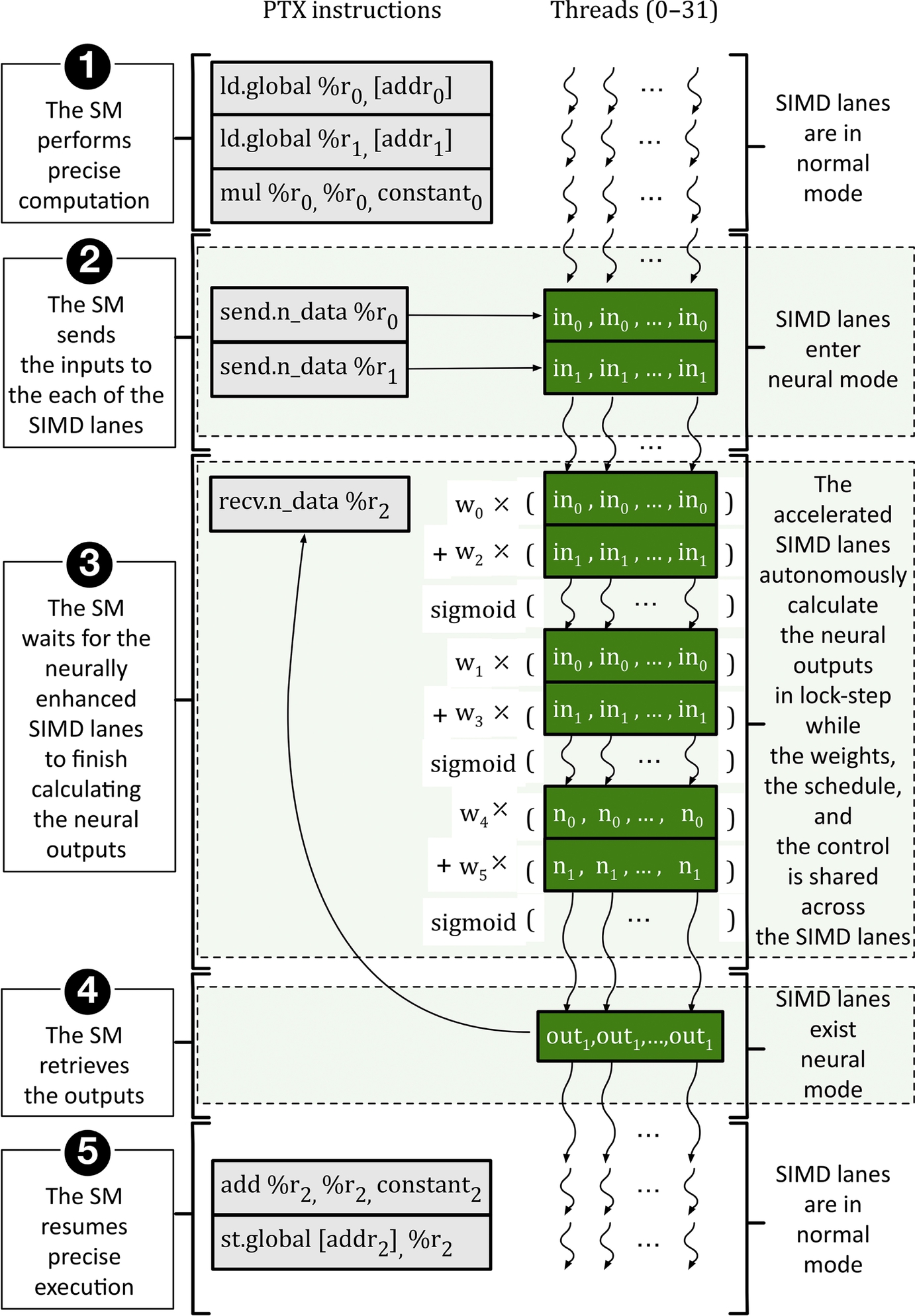
At the same time, the SM issues the recv.n_data instruction. As the output of the neural network is not ready yet, the SM stops issuing the following instructions and waits for the neurally enhanced SIMD lanes to finish computing the neural-network output. In the fourth phase of execution (4) and once the neural-network output is ready, the recv.n_data instruction copies the results of the neural computation from the output buffers to the register file and then, in the fifth phase of execution (5), normal execution resumes. Because there is no control divergence or memory access in the neural mode, this design does not switch the running warp with another warp in the neural mode to avoid the significant overhead of dedicated input/output buffers or control logic per active warp (SMs support 48 ready-to-execute warps in the Fermi architecture).
4.3 Orchestrating Neurally Enhanced SIMD Lanes
For the purpose of efficient execution of neural networks on the neurally enhanced SIMD lanes, the compiler should create a static schedule for the neural computation and arrange the weights in proper order in the FIFO. This schedule and the preordered weights are encoded in the program binary and are preloaded to the Weight FIFO (Fig. 5 (1)) when the program loads for execution. The compiler generates the schedule of the execution using the following steps:
1. The computations for the neurons in each layer are independent on the output of the neurons in the previous layer. As a result, the compiler assigns a unique order to the neurons starting from the first hidden layer down to the output layer. This unique order determines the order of the execution of the neurons. In Fig. 4n0, n1, and n2 show this order.
2. Having the order of the neurons, the compiler generates the order of the multiply-and-add operations for each neuron. The multiply-and-add operations are followed by a sigmoid operation. This schedule is shown in Fig. 7 for the neural network in Fig. 4. The phase (3) of Fig. 6 illustrates how the neurally enhanced SIMD lanes execute this schedule in SIMT mode while sharing the weights and control.

The schedule that is presented in Fig. 7 constitutes most of the accelerator configurations and the order in which the weights will be stored in Weight FIFO ((1) shown in Fig. 5). For each accelerator invocation, SIMD lanes go through these weights in lockstep and perform the neural computation autonomously without engaging the other parts of the SM.
5 Controlling quality trade-offs
All approximation techniques need to expose a quality knob to the compiler and/or runtime system in order to control the quality trade-offs. The knob for the presented neural accelerator is the accelerator invocation rate, which is the fraction of the neurally approximable warps that are offloaded to the neural accelerator. The rest of the neurally approximable warps execute the original precise segment of code and generate exact outputs. Without having a quality-control mechanism, all the warps that contain the approximable segment will go through the neural accelerator which translates into a 100% invocation rate. With a quality-control mechanism, only a fraction of the warps will go through the accelerator. Naturally, the higher the invocation rate, the higher the benefits, and the lower the output quality.
For a given quality target, the compiler predetermines the invocation rate by examining the output quality loss on a held-out evaluation input data set. Starting from 100% invocation rate, the compiler gradually reduces the invocation rate until the quality loss is less than the quality target. During runtime, a quality monitor, similar to the one proposed in SAGE [9], stochastically checks the output quality of the running application and adjusts the invocation rate to make sure that output quality remains below the quality target.
For the purpose of controlling the quality loss, the benefits of using a more sophisticated approach has been investigated [18, 19]. The more sophisticated approach uses another neural network to filter out those invocations of the accelerator that result in significant quality degradation. The empirical study suggested that the simpler approach of reducing the invocation rate provides similar benefits.
6 Evaluation
In this section, we present benefits of the proposed architecture across different bandwidth and accelerator settings [18, 19]. We use a diverse set of applications, cycle-accurate simulation, logic synthesis, and consistent detailed energy modeling.
6.1 Applications and Neural Transformation
Applications
As Table 1 shows, we use a diverse set of approximable GPU applications from the Nvidia SDK [28] and Rodinia [29] benchmark suites to evaluate the integration of the presented neural accelerators within GPU architectures. Moreover, three more applications are added to the mix from different sources [30–32]. As shown in Table 1, the benchmarks are taken from finance, machine learning, image processing, vision, medical imaging, robotics, 3D gaming, and numerical analysis. No benchmark is rejected due to its performance, energy, or quality shortcomings.
Table 1
Applications, Accelerated Regions, Training and Evaluation Data Sets, Quality Metrics, and Approximating Neural Networks
| Digital NPU | ||||||||||||
| Description | Source | Domain | Quality Metric | # of Function Calls | # of oops | # of Ifs/Elses | # of PTX Insts. | Training Input Set | Evaluation Input Set | Neural Network Topology | Quality Loss | |
| binarization | Image binarization | Nvidia SDK | Image Processing | Image diff | 1 | 0 | 1 | 27 | Three 512 × 512 pixel images | Twenty 2048×2048 pixel images | 3 -¿ 4 -¿ 2 -¿ 1 | 8.23% |
| blackscholes | Option pricing | Nvidia SDK | Finance | Avg. rel. error | 2 | 0 | 0 | 96 | 8192 options | 262,144 options | 6 -¿ 8 -¿ 1 | 4.35% |
| convolution | Data filtering operation | Nvidia SDK | Machine learning | Avg. rel. error | 0 | 2 | 2 | 886 | 8192 data points | 262,144 data points | 17 -¿ 2 -¿ 1 | 5.25% |
| inversek2j | Inverse kinematics for 2-joint arm | CUDA-based kinematics | Robotics | Avg. rel. error | 0 | 3 | 5 | 132 | 8192 2D coordinates | 262,144 2D coordinates | 2 -¿ 16 -¿ 3 | 8.73% |
| jmeint | Triangle intersection detection | jMonkey game | 3D Gaming | Miss rate | 4 | 0 | 37 | 2250 | 8192 3D coordinates | 262,144 3D coordinates | 18 -¿ 8 -¿ 2 | 17.32% |
| laplacian | Image sharpening filter | Nvidia SDK | Image processing | Image diff | 0 | 2 | 1 | 51 | Three 512 × 512 pixel images | Twenty 2048×2048 pixel images | 9 -¿ 2 -¿ 1 | 6.01% |
| meanfilter | Image smoothing filter | Nvidia SDK | Machine vision | Image diff | 0 | 2 | 1 | 35 | Three 512 × 512 pixel images | Twenty 2048×2048 pixel images | 7 -¿ 4 -¿ 1 | 7.06% |
| newton-raph | Newton-Raphson equation solver | Likelihood estimators | Numerical analysis | Avg. rel. error | 2 | 2 | 1 | 44 | 8192 cubic equations | 262,144 cubic equations | 5 -¿ 2 -¿ 1 | 3.08% |
| sobel | Edge detection | Nvidia SDK | Image processing | Image diff | 0 | 2 | 1 | 86 | Three 512 × 512 pixel images | Twenty 2048×2048 pixel images | 9 -¿ 4 -¿ 1 | 5.45% |
| srad | Speckle reducing anisotropic diffusion | Rodinia | Medical imaging | Image diff | 0 | 0 | 0 | 110 | Three 512 × 512 pixel images | Twenty 2048×2048 pixel images | 5 -¿ 4 -¿ 1 | 7.43% |

Annotations
As mentioned in Section 2.1, we annotate the CUDA source code of each application using the #pragma directives. We take advantage of these directives to delineate a region within a CUDA kernel that has a fixed number of inputs/outputs and is safe to be approximated. Although it is possible and might also boost the benefits to annotate multiple regions, for the study in this chapter, we annotate only one easy-to-identify region that is frequently executed. We did not make any algorithmic changes to enable neural acceleration.
Table 1 shows the number of function calls, conditionals, and loops of the approximable region of each benchmark. Table 1 illustrates that the approximable regions exhibit a rich and diverse control-flow behavior. As an example, the approximable region in inversk2j has three loops and five conditionals. Other regions similarly have several loops/conditionals and function calls. Among these applications, the approximable region in jmeint has the most complicated control flow with 37 if/else statements. The approximable regions are also diverse in size and vary from small (binarization with 27 PTX instructions) to large (jmeint with 2250 PTX instructions).
Evaluation/training data sets
Table 1 shows the data sets that are used for the benchmarks. The data sets for measuring the quality, performance, and energy are completely disjointed from the ones that are used for training the neural networks. The training inputs are typical representative inputs (such as sample images) that can be found in application test suites. As an example, we use the image of lena, peppers, and mandrill for applications that operate on image data. Since the chosen regions are frequently executed, even a single application input provides a large amount of training data. For instance, a 512 × 512 pixel image generates 262,144 training data elements in sobel.
Neural networks
The “Neural Network Topology” column in Table 1 shows the topology of the neural network that replaces the approximable region of code. As an example, the topology of the neural network for the blackscholes benchmark is 6 → 8 → 1. With this topology, the neural network has six inputs, one hidden layer with eight neurons, and one output neuron. The compiler automatically picks the topology. For training the chosen neural network, we use the 10-fold cross validation technique. As indicated by the topologies of the benchmarks, different applications require different topologies. Consequently, the SM architecture should be reconfigurable and can accommodate different topologies.
Quality
We use application-specific quality metrics, shown in Table 1, to assess the quality of each application’s output after neural acceleration. In all cases, we compare the output of the original precise application to the output of the neurally accelerated application. For blackscholes, inversek2j, newton-raph, and srad which generate numeric outputs, we measure the average relative error. For jmeint which determines whether two 3D triangles intersect, we report the misclassification rate. For convolution, binarization, laplacian, meanfilter, and sobel which produce image outputs, we use the average root-mean-square image difference. In Table 1, the “quality loss” column reports the whole-application quality degradation based on the preceding metrics. This loss includes the accumulated errors due to repeated execution of the approximated region. The quality loss in Table 1 represents the case where all dynamic threads with safe-to-approximate regions are neurally accelerated (i.e., 100% invocation rate).
Even with a 100% invocation rate, the quality loss with neural acceleration is less than 10% except in the case of jmeint. The jmeint application’s control flow is very complex, and the neural network is not capable of capturing all the corner cases to achieve below 10% quality degradation. These results are commensurate with prior work on CPU-based neural acceleration [14, 16]. Prior works on GPU approximation such as SAGE [9] and Paraprox [10] report similar quality losses in the default setting. EnerJ [21] and Truffle [33] show less than 10% loss for some applications and even 80% loss of quality for others. Green [34] and loop perforation [35] show less than a 10% error for some applications and more than 20% for others. Later in this section, we discuss how to use the invocation rate to control the quality trade-offs, and achieve an even lower loss of quality when desired.
To better illustrate the nature of quality loss in GPU applications, Fig. 8 shows the cumulative distribution function (CDF) plot of the final quality loss with respect to the elements of the output. The output of an application is a collection of elements—an image consists of pixels; a vector consists of scalars; and so on. The quality-loss CDF shows that, across all benchmarks, only very few output elements show a large loss; the majority of output elements (from 78% to 100%) show a quality loss of less than 10%.

6.2 Experimental Setup
Cycle-accurate simulations
GPGPU-Sim version 3.2.2 [38] is used for cycle-accurate simulation. The simulator is modified to include the ISA extensions and the extra microarchitectural modifications necessary for the integration of neural accelerators within GPUs. The overhead of ISA extensions for communication with the accelerator are modeled. For baseline simulations that do not include any approximation or acceleration, the unmodified GPGPU-Sim is used. We use one of the GPGPU-Sim’s default configurations that closely models the Nvidia GTX 480 chipset with Fermi architecture. Table 2 summarizes the microarchitectural parameters of the chipset. We run the applications to completion. We use NVCC 4.2 with -O3 to enable aggressive compiler optimizations. Moreover, we optimize the number of thread blocks and number of threads-per-block of each kernel for the simulated hardware.
Table 2
GPU Microarchitectural Parameters
System overview: No. of SMs: 15, warp size: 32 threads/warp; Shader core config: 1.4 GHz, GTO scheduler [36], 2 schedulers/SM; Resources/SM: No. of warps: 48 warps/SM, No. of registers: 32,768; Interconnect: 1 crossbar/direction (15 SMs, 6 MCs), 700 MHz; L1 data cache: 16 KB, 128B line, 4-way, LRU; Shared memory: 48 KB, 32 banks; L2 unified cache: 768 KB, 128B line, 16-way, LRU; Memory: 6 GDDR5 memory controllers, 924 MHz, FR-FCFS [37]; Bandwidth: 177.4 GB/s.
Energy modeling and overhead
For the purpose of measuring the GPU energy usage, we use GPUWattch [39], which is integrated with GPGPU-Sim. To measure the neural accelerator energy usage, we benefit from an event log that is generated during the cycle-accurate simulation. The energy evaluations are based on a 40 nm process node with 1.4 GHz clock frequency. Neural acceleration requires the following changes to the SM and SIMD lanes and are modeled using McPAT [40] and CACTI 6.5 [41]. In each SM, we add a 2 KB dual-port weight FIFO. The input/output FIFOs are 256 bytes per SIMD lane. The sigmoid look-up table which is added to each SIMD lane contains 2048 32-bit entries. Because GPUWattch uses McPAT and CACTI, we benefit from a unified and consistent framework for energy measurement.
6.3 Experimental Results
Performance and energy benefits
Fig. 9 shows the whole application speedup when all the invocations of the approximable region are accelerated with the neural accelerator. The remaining part (i.e., the nonapproximable region) is executed normally. The results are normalized to the baseline where the entire application is executed on the GPU with no acceleration. The highest speedup is observed for newton-raph (14.3×) and inversek2j (9.8×), where the bulk of execution time is spent on approximable parts (see Fig. 1). The lowest speedup is observed for blackscholes and srad (about 2% and 5%) which are bandwidth-hungry applications. While a considerable fraction of the execution time in blackscholes and srad is spent in the approximate regions (see Fig. 1), the speedup of accelerating these two applications is modest. This is because these applications use most of the off-chip bandwidth, even when they run on a GPU without any acceleration. Because of bandwidth limitation, neural acceleration cannot reduce the execution time as most of the time is spent on loading data from memory. We study the effect of increasing the off-chip bandwidth on these two applications and show that with reasonable improvement in bandwidth, even these benchmarks observe significant benefits. On average, the evaluated applications see a 2.4× speedup through neural acceleration.

Fig. 10 shows the energy reduction for each benchmark as compared to the baseline where the whole benchmark is executed on a GPU without acceleration. Similar to the speedup, the highest energy saving is achieved for inversek2j (18.9×) and newton-raph (14.8×), where the bulk of the energy is consumed for the execution of approximable parts (see Fig. 1). The lowest energy saving is obtained on jmeint (30%) as for this application the fraction of energy consumed on approximable parts is relatively small (see Fig. 1). Unlike the speedup, we see that all applications including those that are bandwidth-hungry benefit from neural acceleration to reduce the energy usage. On average, the evaluated applications see a 2.8× reduction in energy usage.

The quality loss when all the invocations of the approximable region are executed on neural accelerators (i.e., the highest quality loss) is shown in Table 1 (labeled “quality loss”). We study the effects of the quality-control mechanism on trading performance and energy savings for better quality later in this section.
Area overhead
To estimate the area overhead, we synthesize the sigmoid unit using Synopsys Design Compiler and NanGate 45 nm Open Cell library, targeting the same frequency as the SMs. We extract the area of the buffers and FIFOs from CACTI. Overall, the added hardware requires about 0.27 mm2. We estimate the area of the SMs by inspecting the die photo of GTX 480 that implements the Fermi architecture. Each SM is about 22 mm2, and the die area is 529 mm2 with 15 SMs. The area overhead per SM is approximately 1.2%, and the total area overhead is 0.77%. The low area overhead is because the described architecture uses the same ALUs that are already available in each SIMD lane, shares the weight buffer across the SIMD lanes, and implements the sigmoid unit as a read-only look-up table, enabling the synthesis tool to optimize its area. This low area overhead confirms the scalability of the mentioned design.
Opportunity for further improvements
To explore the opportunity for further improving the execution time by making the neural accelerator faster, see Fig. 11, which shows the time breakdown of approximable and nonapproximable regions of applications when applications run on GPU (no acceleration) and neurally accelerated GPU (NGPU), normalized to the case where the application runs on GPU (no acceleration). As Fig. 11 shows, NGPU is effective at significantly reducing the time that is spent on the approximable region for all but two applications: blackscholes and srad. These two applications use most of the bandwidth of the GPU and, consequently, do not benefit from the accelerators due to the bandwidth wall. The rest of the applications significantly benefit from the accelerators. On some applications (e.g., binarization, laplacian, sobel), the execution time of the approximable region on NGPU is significantly smaller than the execution time of the nonapproximable region. Hence no further improvement is possible with faster accelerators. For the rest of the applications, the execution time of the approximable region on NGPU, although considerably reduced, is comparable to and sometimes exceeds (e.g., inversek2j) the execution time of the nonapproximable region. For such applications, there is a potential to further reduce the execution time with faster accelerators.
We similarly study the opportunity to further reduce the energy usage with more energy-efficient accelerators. Fig. 12 shows the energy breakdown between approximable and nonapproximable regions when applications run on GPU and NGPU, normalized to the case where applications run on GPU. The results in Fig. 12 clearly show that neural accelerators are effective at reducing the energy usage of applications when executing the approximable region. For many of the applications, the energy that is consumed for running the approximable region is modest as compared to the energy that is consumed for running the nonapproximable region (e.g., blackscholes, convolution, jmeint). For these applications, a more energy-efficient neural accelerator may not bring further energy savings. However, there are some applications, such as binarization, laplacian, and sobel, for which the fraction of energy that is consumed on neural accelerators is comparable to the fraction of energy consumed on nonapproximable regions. For these applications, further energy saving is possible with a more energy-efficient implementation of neural accelerators (e.g., analog neural accelerators [14]).

Sensitivity to accelerator speed
To study the effects of an accelerator’s speed on the performance gains, in this section we vary the latency of neural accelerators and measure the overall speedup. Fig. 13 shows the results of this experiment. We decrease the delay of the default accelerators by a factor of 2 and 4 and also include an ideal neural accelerator with zero latency. Moreover, we show the speedup numbers when the latency of the default accelerators increases by a factor of 2, 4, 8, and 16. Unlike Fig. 11 that suggests having faster accelerators results in performance improvement for some applications, Fig. 13 shows virtually no speedup benefits as a result of making neural accelerators faster beyond what they offer in the default design. Even making the neural accelerators slower by a factor of 2 does not considerably change the speedup numbers. Slowing down the neural accelerators by a factor of 4, many applications show a loss in a performance (e.g., laplacian).

 faster) shows the total application speedup when the neural accelerator has zero delay.
To illustrate the previously mentioned behavior, Fig. 14 shows the bandwidth usage of GPU and NGPU across all applications. While on the baseline GPU, only two applications require more than 50% of the off-chip bandwidth (i.e., blackscholes and srad), on NGPU, many applications need more than 50% of the off-chip bandwidth (e.g., inversek2j, jmeint, newton-raph). Because applications run faster with neural accelerators, the rate at which they access data increases The high rate of accessing data puts pressure on off-chip bandwidth. This phenomenon shifts the bottleneck of execution from computation to data delivery. With the default accelerators, computation is no longer the major bottleneck. Consequently, speeding up thread execution beyond a certain point has a marginal effect on the overall execution time. Even increasing the accelerator speed by a factor of 2 (e.g., by adding more multiply-and-add units) has a marginal effect on the execution time. This insight has been leveraged for the simplification of the accelerator design and the reuse of available ALUs in the SMs as described is Section 4.1.

Sensitivity to off-chip bandwidth
To study the effect of off-chip bandwidth on the benefits of NGPU, we increase the off-chip bandwidth up to 8× and report the performance numbers. Fig. 15 shows the speedup of NGPU with 2×, 4×, and 8× bandwidth over the baseline NGPU (i.e., 1× bandwidth) across all benchmarks. Because NGPU is bandwidth-limited for many applications (see Fig. 14), we expect a considerable improvement in performance as the off-chip bandwidth increases. Indeed, Fig. 15 shows that bandwidth-hungry applications (i.e., blackscholes, inversek2j, jmeint, and srad) show a speedup of 1.5× when we double the off-chip bandwidth. After doubling the off-chip bandwidth, no application remains bandwidth-limited. As a result, increasing the off-chip bandwidth to 4× and 8× has little effect on performance. It may be possible to achieve the 2× extra bandwidth using data compression [42] with few changes to the architecture of existing GPUs. Although technologies like 3D DRAM that offer significantly more bandwidth (and lower access latency) can be useful, they are not necessary for providing the off-chip bandwidth requirements of NGPU for the range of applications that we studied. However, even without any of these likely technological advances (compression or 3D stacking), the NGPU provides significant benefits across most of the applications.

Controlling quality trade-offs
To illustrate the effect of the quality-control mechanism, Fig. 16 shows the energy-delay product of NGPU normalized to the energy-delay product of the baseline GPU (without acceleration) when the output quality loss changes from 0% (i.e., no acceleration) to 10%. The quality-control mechanism enables navigating the trade-off between the quality loss and the gains. All applications show declines in benefits when the invocation rate decreases (i.e., output quality improves). Because of the Amdahl’s Law effect, the applications that spend more than 90% of their execution in the approximable region (inversek2j and newton-raph) show larger declines in benefits when the invocation rate decreases. However, even with a 2.5% quality loss, the average speedup is 1.9× and the energy savings is 2.1×.

Comparison with prior CPU neural acceleration
Prior work [13] has explored improving CPU performance and energy efficiency with NPUs. As NPUs offer considerably higher performance and energy efficiency with CPUs, we compare NGPU to CPU + NPU and GPU + NPU. For the evaluation, we use a MARSSx86 cycle-accurate simulator for the single-core CPU simulations with a configuration that resembles Intel Nehalem (3.4 GHz with 0.9 V at 45 nm) and is the same as the setup used in the most recent NPU work [14].
Fig. 17 shows the application speedup and Fig. 18 shows the application energy reduction with CPU, GPU, GPU + NPU, and NGPU over CPU + NPU. Even without using neural acceleration, a GPU provides significant performance and efficiency benefits over NPU-accelerated CPU by leveraging data-level parallelism. A GPU offers 5.6× average speedup and 3.9× average energy reduction as compared to CPU + NPU. A GPU enhanced with neural accelerators (NGPU) increases the average speedup and energy reduction to 13.2× and 10.8×, respectively. Moreover, as GPUs already exploit data-level parallelism, an NGPU offers virtually the same speedup as the area-intensive GPU + NPU. However, accelerating GPU with the NPU design imposes a 31.2% area overhead while the NGPU imposes just 1.2% per SM. A GPU with area-intensive NPU (GPU + NPU) offers 17.4% less energy benefits as compared to NGPU mostly due to more leakage. In summary, NGPU offers the highest level of performance and energy efficiency across the examined benchmarks with the modest area overhead of approximately 1.2% per SM.


7 Related work
Recent work explored a variety of approximation techniques that include: (a) approximate storage designs [43, 44] that trade quality of data for reduced energy [43] and longer lifetime [44], (b) voltage over-scaling [33, 45, 46], (c) loop perforation [35, 47, 48], (d) loop early termination [34], (e) computation substitution [9, 12, 34, 49], (f) memoization [10, 11, 50], (g) limited fault recovery [47, 51–55], (h) precision scaling [21, 56], (i) approximate circuit synthesis [24, 57–62], and (j) neural acceleration [13–19].
What has been presented in this chapter falls in the last category with the focus being the integration of neural accelerators into GPU throughput processors [18, 19]. Some recent work on neural acceleration focuses on single-threaded CPU code acceleration by either loosely coupled neural accelerators [15–17, 63, 64] or tightly coupled ones [13, 14]. Grigorian et al. study the effects of eliminating control-flow divergence by converting SIMD code to software neural networks with no hardware support [2]. However, these pieces of work do not explore tight integration of neural hardware in throughput processors and do not study the interplay of data-parallel execution and hardware neural acceleration. Prior to this work, the benefits, limits, and challenges of integrating hardware neural acceleration within GPUs for many-thread data-parallel applications was unexplored.
There are several other approximation techniques in the literature that can or have been applied to GPU architectures. Loop perforation [35] periodically skips loop iteration for gains in performance and energy efficiency. Green [34] terminates loops early or substitute compute-intensive functions with simpler, lower quality versions that are provided by the programmer. Relax [51] is a compiler/architecture system for suppressing hardware fault recovery in approximable regions of code, exposing these errors to the application. Fuzzy memoization foregoes invoking a floating-point unit if the inputs are in the neighborhood of previously seen inputs. The result of the previous calculation is reused as an approximate result. Arnau et al. use hardware memoization to reduce redundant computation in GPUs [11]. Sartori et al. propose a technique that mitigates branch divergence by forcing the divergent threads to execute the most popular path [12]. In case of memory divergence, they force all the threads to access the most commonly demanded memory block. SAGE [9] and Paraprox [1] perform compile-time static code transformations on GPU kernels that include data compression, profile-directed memoization, thread fusion, and atomic operation optimization. Our quality-control mechanism takes inspiration from the quality control in these two pieces of work.
In contrast, in this chapter, we describe a hardware approximation technique that integrates neural accelerators within the pipeline of the GPU cores. In our design, we aim at minimizing the pipeline modifications and utilizing existing hardware components. Specifically, this work explores the interplay between data parallelism and neural acceleration and studies its limits, challenges, and benefits.
8 Conclusion
Many of the emerging applications that can benefit from GPU acceleration are amenable to inexact computation. We exploited this opportunity by integrating an approximate form of acceleration, neural acceleration, within GPU architectures. The NGPU architecture provides significant performance and energy-efficiency benefits while providing reasonably low hardware overhead (1.2% area overhead per SM). The quality-control knob and mechanism also provided a way to navigate the trade-off between the quality and the benefits in efficiency and performance. Even with as low as only a 2.5% quality loss, the NGPU architecture provides average speedup of 1.9× and average energy savings of 2.1×. These benefits are more than 10× in several cases. These results suggest that hardware neural acceleration for GPU throughput processors can be a viable approach to significantly improve their performance and efficiency.