Augmented Block Cimmino Distributed Algorithm for solving tridiagonal systems on GPU
Y.-C. Chen; C.-R. Lee National Tsing Hua University, Hsinchu City, Taiwan
Abstract
Tridiagonal systems appear in many scientific and engineering problems, such as Alternating Direction Implicit methods, fluid simulation, and Poisson equation. This chapter presents the parallelization of the Augmented Block Cimmino Distributed method for solving tridiagonal systems on graphics processing units (GPUs). Because of the special structure of tridiagonal matrices, we investigate the boundary padding technique to eliminate the execution branches on GPUs. Various performance optimization techniques, such as memory coalescing, are also incorporated to further enhance the performance. We evaluate the performance of our GPU implementation and analyze the effectiveness of each optimization technique. Over 24 times speedups can be obtained on the GPU as compared to speedups on the CPU version.
Keywords
Tridiagonal solver; GPU; Parallel algorithm; Numerical linear algebra; Performance optimization
1 Introduction
A tridiagonal matrix has nonzero elements only on the main diagonal, the diagonal upon the main diagonal, and the diagonal below the main diagonal. This special structure appears often in scientific computing and computer graphics [1, 2]. Because many of them require real-time execution, the solver must compute the result quickly as well as correctly. Many parallel algorithms for solving a tridiagonal system have been proposed [2–6]. These algorithms can give answers with superior accuracy and short execution time. Many applications or open-source tridiagonal matrix solvers are based on these algorithms, such as Alternating Direction Implicit [1] and cuSPARSE package [7].
The Augmented Block Cimmino Distributed (ABCD) method [8] is a new type of algorithm to solve linear systems. It partitions the matrix into block rows and constructs the augmented matrices to make each block row orthogonal. Although the augmentation increases the problem size, the orthogonalization makes the parallelization easy, since each augmented block row can be solved independently. Moreover, because of the orthogonal property, each block row can be solved stably without pivoting.
This chapter describes the implementation and performance optimization techniques of the ABCD algorithm for solving tridiagonal systems on a graphics processing unit (GPU). Although ABCD algorithm can be paralleled easily at the coarse-grained level, for multicore devices such as a GPU, fine-grained parallelization is more important. The major problem is that the operations in the block row solver are few, so the optimization of each step in the implementation is critical to the overall performance.
The rest of the chapter is organized as follows: Section 2 introduces the ABCD method for solving tridiagonal systems. Section 3 describes the details of GPU implementation and performance optimization techniques. Section 4 presents the experimental results. The conclusion is given in the last section.
2 ABCD Solver for tridiagonal systems
The ABCD method is a redesigned block Cimmino algorithm, which is an iterative method for solving large linear least square problems. Let A be an m × n matrix and b an m vector. The linear least square problem is to solve x
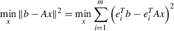
where ei is the ith column of an m × m identity matrix I. The preceding question can be written in the block form,

where Ei is the ith block column of the identity matrix. This is equivalent to partitioning the matrix A into p equal-sized row blocks, as well as the vector b. Fig. 1 shows a picture of the partition. If we let bi = EiTb and ![]() , the preceding equation becomes
, the preceding equation becomes


The original block Cimmino method approximates the solution of each row block in parallel, and iteratively makes the approximations converge to the solution.
If each block row Ai is orthogonal to each other, which means ![]() for i≠j, the exact solution can be obtained in one iteration. Of course, most matrices do not possess such a property. However, we can augment the matrix so that the augmented matrix has this property. For instance, suppose the original matrix A has four row blocks, A = (A1A2A3A4)T, in which case, we can construct an augmented matrix
for i≠j, the exact solution can be obtained in one iteration. Of course, most matrices do not possess such a property. However, we can augment the matrix so that the augmented matrix has this property. For instance, suppose the original matrix A has four row blocks, A = (A1A2A3A4)T, in which case, we can construct an augmented matrix
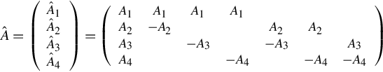
in which ![]() if i≠j. In the preceding example, the matrix size is increased seven times by augmentation.
if i≠j. In the preceding example, the matrix size is increased seven times by augmentation.
Augmentation could be small if a matrix has some special structures, such as tridiagonal matrices. Here is an example. Let A be a 9 × 9 tridiagonal matrix, and let p = 3, which means matrix A is partitioned into three row blocks.

To make each block row orthogonal to each other, we can simply augment the matrix as follows:

Because only few elements are overlapped between consecutive row blocks in a tridiagonal matrix, only 2(p − 1) column augmentation should be added for p partitions.
Suppose Ax = b is the original tridiagonal system to solve, where A is an m × m tridiagonal matrix, x is the unknown, and b is an m vector. The augmented system can be written as

The solution of x will be the same solution as the original problem. The only problem is that the augmented row block (O I) is not orthogonal to other row blocks in (A C), which makes parallelization difficult. This can be solved by projecting (O I) to the orthogonal subspace of (A C). Let ![]() , and
, and ![]() be the block rows of
be the block rows of ![]() . The oblique projector of
. The oblique projector of ![]() is
is

Therefore we can construct the appending matrix
and the augmented right-hand side
The augmented system becomes
The solution of Eq. (3) is
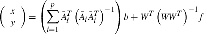
whose upper part x is the solution of the original system.
The ABCD method is summarized in Algorithm 1.
Algorithm 1
Augmented Block Cimmino Distributed Method
1. Determine partition size p and construct augmented matrix C.
2. Compute ![]() ,
, ![]() , fi = (O I)ui,
, fi = (O I)ui,
and ![]() for i = 1, …, p in parallel.
for i = 1, …, p in parallel.
3. Compute ![]() ,
, ![]() ,
, ![]() ,
,
and 
4. Solve Sz = f and compute v = Wz.
5. Return the upper part of u + v.
3 GPU implementation and optimization
Here we present the details of the GPU implementation of the ABCD method for solving tridiagonal systems and the performance optimization techniques.
3.1 QR Method and Givens Rotation
The major computation in Algorithm 1 is the calculation of
where ![]() is a block row of the augmented matrix. Each block row has three nonzero diagonal elements and few augmented elements. However, the calculation using Eq. (5) has some drawbacks. First, although the matrix is quite sparse, the direct calculation still iterates many times, especially the calculation of
is a block row of the augmented matrix. Each block row has three nonzero diagonal elements and few augmented elements. However, the calculation using Eq. (5) has some drawbacks. First, although the matrix is quite sparse, the direct calculation still iterates many times, especially the calculation of ![]() . If
. If ![]() is an k × q matrix,
is an k × q matrix, ![]() is an k × k matrix. Because
is an k × k matrix. Because ![]() is almost a tridiagonal matrix,
is almost a tridiagonal matrix, ![]() will be a band matrix with five diagonals. Second, the direct calculation of oblique projector using Eq. (5) is numerically unstable [9, Chapter 14], even with some pivoting strategies. A better choice is the QR method.
will be a band matrix with five diagonals. Second, the direct calculation of oblique projector using Eq. (5) is numerically unstable [9, Chapter 14], even with some pivoting strategies. A better choice is the QR method.
The QR method first decomposes the matrix ![]() into the product of an orthogonal matrix Qi and an upper triangular matrix Ri,
into the product of an orthogonal matrix Qi and an upper triangular matrix Ri, ![]() . Based on that, Eq. (5) can be simplified as
. Based on that, Eq. (5) can be simplified as
and
assuming ![]() or Ri is of full rank. As can be seen, the formulas in Eqs. (6), (7) are much simpler and cleaner than that in Eq. (5).
or Ri is of full rank. As can be seen, the formulas in Eqs. (6), (7) are much simpler and cleaner than that in Eq. (5).
There are several algorithms to carry out the QR decomposition [10, Chapter 5]. The most suitable one for matrix ![]() is the Givens rotation, because
is the Givens rotation, because ![]() , a tridiagonal matrix, is very close to the upper triangular matrix Ri structurally, except for one subdiagonal and few augmented elements, and the Givens rotation method annihilates those nonzero elements one by one using rotation matrices. A rotation matrix for a two-vector v = (a b)T is
, a tridiagonal matrix, is very close to the upper triangular matrix Ri structurally, except for one subdiagonal and few augmented elements, and the Givens rotation method annihilates those nonzero elements one by one using rotation matrices. A rotation matrix for a two-vector v = (a b)T is

where c = a/d, s = b/d, and ![]() . By premultiplying G to v,
. By premultiplying G to v, ![]() . Note that G is a orthonormal matrix, and it preserves the length of the multiplicand, which means v and Gv have the same length.
. Note that G is a orthonormal matrix, and it preserves the length of the multiplicand, which means v and Gv have the same length.
The QR decomposition by Givens rotation uses the diagonal and subdiagonal elements to create rotation matrices to brings zeros to the subdiagonal. The final Q matrix can be obtained by cumulating the rotation matrices.
Table 1 compares the operation counts of the Givens rotation and the direct method using Eq. (5). The size of ![]() is n × k, and the size of Ci is ℓ × k. The operation count of the direct method is based on the spare matrix multiplication and Gaussian elimination for band matrix. As can be seen, the operation count of Givens rotation is almost half in the computation of Si, compared to that of the direct method.
is n × k, and the size of Ci is ℓ × k. The operation count of the direct method is based on the spare matrix multiplication and Gaussian elimination for band matrix. As can be seen, the operation count of Givens rotation is almost half in the computation of Si, compared to that of the direct method.
3.2 Sparse Storage Format
Because A is tridiagonal, which is extremely sparse, a special storage format should be considered to reduce the used memory. A simple format of a tridiagonal matrix is to use three vectors to store the nonzero elements. In addition to that, we also need to consider the storage for intermediate results, such as the storage for matrix Q and matrix R.
Based on those requirements, we designed a 5n array as the major storage format, as shown in Fig. 2. Matrix A can be stored in the first three n vectors. Matrix R is also a tridiagonal matrix, whose nonzeros are all above the main diagonal. After the QR decomposition, matrix R can use the same space as matrix A’s since A is no longer needed in the computation. Matrix Q is a block diagonal matrix. To store it may take too much space. Alternatively, we keep the Q matrix in the decomposed form and store the rotation matrices Gi. Since each Gi only has two parameters, we only need two elements to store each Gi. So the last two vectors are used to store the rotation matrix Gi. When the matrix Q is required in computation, such as Eq. (6), we multiply those Gi by the multiplicand directly.

3.3 Coalesced Memory Access
We reformat the matrix storage to improve the performance on the GPU. As suggested in Ref. [11], the data accessed by threads within a block should be successively stored because threads in a thread-block read or store simultaneously. Successively stored data allows coalesced memory access on the GPU, which can read/write 128 or more elements simultaneously, depending on the GPU hardware structure.
The original data storage format that stores the adjacent tridiagonal elements successively in memory cannot make coalesced memory access. Therefore we modify to the storage method so that the element k in the ith partition is before the element k in i − 1th partition and followed by the element k in the i + 1th partition.
Fig. 3 shows an example. There are eight elements, and each block has two threads. The number of partitions is two, which means that each thread controls 8/2 = 4 elements. Elements are reformatted based on the number of threads in a block. If thread 1 needs to access elements from 1 to 4 and thread 2 needs to access elements from 5 to 8, we place elements 1 and 5 together, 3 and 6 together, and so on. The new storage lets the threads in a block access data simultaneously. Although the data reformatting also costs time, this technique fulfills the coalescing requirement on the GPU and contributes to a higher memory accessing efficiency in the following steps. Experimental results are shown in the next section.

3.4 Boundary Padding
One problem of single instruction multiple data architecture, such as GPU, is the branch divergence, which means a group of threads sharing the same program counter have different execution paths. On a Compute Unified Device Architecture (CUDA) core, threads from a block are bundled into fixed-size warps for execution. Threads within a warp follow the same instruction synchronously. If a kernel function encounters an if-then-else statement that some threads evaluate to true while others to false, a branch divergence occurs. Because of the restriction that threads in a warp cannot diverge to different conditions, warp deactivates the false conditioned threads and proceeds to the true condition, and then reverses condition. In other words, the branch divergence serializes all the possible execution paths, which can really hurt a GPU’s performance.
In the ABCD algorithm, the branch divergence occurs on the boundary process, which needs to handle different data. To solve the problem, we proposed the boundary padding technique, which adds unnecessary paddings and uses additional memory spaces for those threads with different execution on the GPU. The boundary padding technique ensures that all the threads in the same warp perform the same operations at any moment, which eliminates branch divergence.
3.4.1 Padding of the augmented matrix
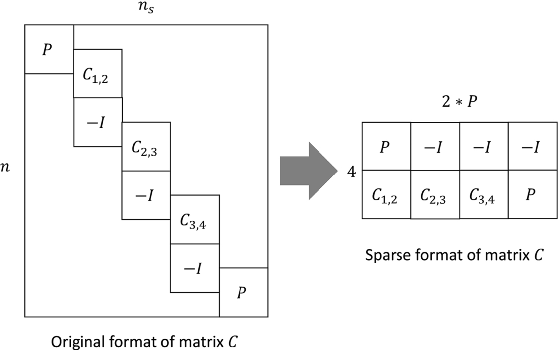
Fig. 4 shows that the augmentations for the top and bottom partitions are different from those of the middle partitions, because they lack either Ci, j or negative identity − I, which will lead to divergences. Our implementation adds zero elements to the top and bottom parts of the augmented matrix. Those zero elements have no actual influence on the final solution. The padding does not cost extra storage. Fig. 5 shows how those padding are stored in a compact format.

3.4.2 Padding for Givens rotation
During the rotation steps, the first partition of ABCD is different from other partitions. It rotates to middle and lower diagonal, while other partitions rotate to lower and below the lower diagonal, which leads to branches. To reduce the branches, we add redundant elements to the first partition. In other words, the first partition will further rotate to the lower diagonal and the diagonal below the lower diagonal. This technique doubles the work of the first partition but unifies the work among all threads. In our experiment results, the total time of calculating the Givens rotations can be reduced to half of the original time. Fig. 6 shows the padding before and after the padding on the first partition.

4 Performance evaluation
We first compare the performance of CPU and GPU implementation. Then we evaluate the speedup before and after applying the performance optimization techniques. The testing matrices are collected from Matlab standard libraries, Toeplitz matrices, and random generations.
The experimental platform is equipped with Intel Xeon CPU E5-2670 v2, which is of 2.50 GHz. The used GPU is NVIDIA Tesla K20m. The operating system is CentOS 6.4, and the NVIDIA Driver is 340.65.
4.1 Comparison With CPU Implementation
Fig. 7 shows the comparison between our implementations of the ABCD algorithm on the GPU and on CPU. The dataflow are the same for all the functions. The CPU version is implemented in C; the GPU version is implemented in CUDA. As shown in Table 2, the calculation of two implementations are similar if the matrix size is smaller than 217 because we have to load data onto GPU memory before starting calculation. The overload caused by moving the data is large compared to calculation time. But the CPU calculation time nearly doubles when the dimension of the matrix doubles, while GPU calculation time increases only a little. The difference is because of GPU’s architecture. If the dimension rises to 4 million, a 24.15 times speedup can be obtained by using GPU. The speedup of difference between a matrix size of 2 million and 4 million is small because we believe that GPU reaches the hardware limits.


4.2 Speedup by Memory Coalescing
Table 3 lists the speedups of different kernels made by the coalescing storage format, as described in Section 3.3. The matrix size is 4 million. The speedup is calculated by the ratio of the time without coalesced format and the time with coalesced format. Coalesced format can attribute to over five times speedup for solving ![]() with multiple right-hand sides.
with multiple right-hand sides.
Table 3
Speedup by Coalesced Memory Access
| Kernel (Functionality) | Speedup (Original/Coalesced) |
| Assign augmented matrix | 1.180 |
| Create Givens rotation | 1.519 |
| Apply Givens rotation | 1.750 |
| Solve | 1.959 |
| Solve | 5.082 |
| Calculate u and f | 2.319 |
| Calculate matrix S | 1.873 |
| Solve S−1 | 3.464 |
There are many factors influencing the possible speedup. The major one is the size of memory accessed by the kernel. More memory accesses give a larger speedup. When the data size is small, its effectiveness is limited. As shown in Table 3, only a 1.15× speedup can be obtained for the task of assigning an augmented matrix. Another reason is the data access pattern. With the original data format, increasing the number of threads cannot accelerate the performance. But with a coalesced data format, doubling the number of threads reduces almost half of the execution time. This is because the bottleneck of the program using the original data format is memory access. More threads do not help to improve the performance. On the other hand, with a coalesced data format, the memory access is no longer the performance bottleneck. So other performance-tuning techniques can take effect. The other factors influencing the speedups include memory size, total number of threads, and the operations on the memory.
4.3 Boundary Padding
Although padding adds useless work to some threads, all threads can perform the same instructions simultaneously, which increases the overall performance.
Table 4 shows the speedup of the boundary padding technique. The speedup comes from two major factors. First, the boundary padding technique reduces the branch divergence because all the threads have the same execution path. Second, the boundary padding technique increases the coalesced memory access, since the memory access pattern is unified.
Table 4
Speedup by Boundary Padding
| Kernel (Functionality) | Speedup (Times) |
| Add padding to the augmented matrix C | 1.254 |
| Add padding for Givens rotation (create rotation) | 2.548 |
| Add padding for Givens rotation (apply rotation) | 1.898 |
The padding for a Givens rotation can not only improve the performance of creating the rotation matrix but also accelerate the kernel that applies the Givens rotations, as shown in the results in Table 4.
5 Conclusion and future work
We present the GPU implementation of the ABCD algorithm, which provides a totally new aspect of parallel algorithm using augmentation. We focus on the problem of solving tridiagonal systems. Because of the special structure of tridiagonal matrices, two performance optimization techniques are proposed to accelerate the GPU implementation. The first is the memory coalesced data format, which significantly reduces the memory access time. The second one is the boundary padding, which adds useless data to unify the execution paths, and can effectively reduce the branches’ divergence on the GPU. Experiments show that a speedup of more than 24 times can be obtained by using the GPU implementation.
Several future directions are worthy of investigation. First, the ABCD algorithm can be applied to general sparse matrices, but the matrix structure will be varied. How to handle the general sparse matrices effectively is a question. Second, here we only consider the parallelization on single-GPU platform. For better scalability, a multi-GPU platform or even heterogeneous platforms that hybrid various devices should be considered. How to design and optimize the algorithms is an interesting problem.