
Energy and power considerations of GPUs
J. Coplin; M. Burtscher Texas State University, San Marcos, TX, United States
Abstract
This chapter discusses the impact of different algorithm implementations, program inputs, core and memory clock frequencies, and source-code optimizations on the energy consumption, power draw, and performance of a modern compute GPU. We distinguish between memory- and compute-bound codes as well as regular and irregular codes and point out behavioral differences between these classes of programs. We present examples of software approaches to alter the energy, power, and runtime of GPU kernels and explain how they can be employed by the end user to improve energy efficiency.
Keywords
General-purpose GPU computing; Power-aware computing; Energy efficiency; Performance evaluation; Source-code optimization
1 Introduction
GPU-based accelerators are widely used in high-performance computing (HPC) and are quickly spreading in PCs and even handheld devices as they often provide higher performance and better energy efficiency than multicore CPUs. For example, in HPC environments, large energy consumption and the required cooling due to the resulting heat dissipation are major cost factors. To reach exascale computing, a 50-fold improvement in performance per watt is needed by some estimates [1]. Moreover, in all types of handheld devices, such as tablets and smartphones, battery life is a key concern.
For these and other reasons, power-aware and energy-efficient computing has become increasingly important. Although many hardware optimizations for reducing power have been proposed or are already in use, software techniques are lagging behind, particularly techniques that target accelerators like GPUs. To be able to optimize the power and energy efficiency of GPU code, it is essential to have a good understanding of the power-draw and energy-consumption behavior of programs on the one hand and of software techniques to manipulate performance, power, and energy on the other hand. Hence this chapter comprises two parts, one on power profiling and the other on improving GPU power and energy using various approaches that an end user can apply.
There are many challenges to studying energy efficiency and power draw on GPUs, not the least of which is trying to accurately measure the power draw. Current GPU-internal power sensors are set to sample at under 100 Hz, so the small-scale power behavior of programs may not be observable. In contrast, some external power sensors sample at rates many times that of internal sensors but may mix in the power from other hardware components and make it more difficult to correlate the measurements with the activities of the GPU code.
It is well known that code optimizations can improve GPU performance a great deal, but their impact on energy and power is less clear. Some studies report a one-to-one correspondence between runtime and energy [2–4]. These studies tend to focus on regular programs and primarily vary the program inputs, not the code itself. However, there are software techniques that improve energy or power substantially more than runtime. This chapter illustrates, on several compute- and memory-bound as well as regular and irregular codes, by how much source-code optimizations, changes in algorithms and their implementations, and GPU clock-frequency adjustments can help make GPUs more energy-efficient.
1.1 Compute- and Memory-Bound Codes on GPUs
A piece of code is said to be compute-bound when its performance is primarily limited by the computational throughput of the processing elements. Compute-bound code typically does a great deal of processing on each piece of data it accesses in the main memory. In contrast, the performance of memory-bound code is primarily limited by the data-transfer throughput of the memory system. Memory-bound code does relatively little processing on each piece of data it reads from the main memory.
1.2 Regular and Irregular Codes on GPUs
By regular and irregular programs, we are referring to the behavior of the control flow and/or memory-access patterns of the code. In regular code, most of the control flow and the memory references are not data-dependent. Matrix-vector multiplication is a good example. Based only on the input size and the data-structure starting addresses, but without knowing any values of the input data, we can determine the dynamic behavior of the program on an in-order processor, that is, the memory reference stream and the conditional branch decisions. In irregular code, the input values determine the program’s runtime behavior, which therefore cannot be statically predicted and may be different for different inputs. For instance, in a binary search tree implementation, the values and the order in which they are processed affect the shape of the search tree and the order in which it is built.
Irregular algorithms tend to arise from the use of complex data structures such as trees and graphs. For instance, in graph applications, memory-access patterns are usually data-dependent since the connectivity of the graph and the values on nodes and edges may determine which nodes and edges are touched by a given computation. This information is usually not known at compile time and may change dynamically even after the input graph is available, leading to uncoalesced memory accesses and bank conflicts. Similarly, the control flow is usually irregular because branch decisions differ for nodes with different degrees or labels, leading to branch divergence and load imbalance. As a consequence, the power draw of irregular GPU applications can change over time in a seemingly erratic manner.
2 Evaluation methodology
2.1 Benchmark Programs
In order to study GPU performance, energy, and power, we utilize programs from the LonestarGPU v2.0 [5], Parboil [6], Rodinia v3.0 [7], and SHOC v1.1.2 [8] benchmark suites as well as a few programs from the CUDA SDK v6.0 [9]. Each program and the used inputs are explained in the “Appendix” section.
2.2 System, Compiler, and Power Measurement
We performed all measurements presented in this chapter on a Nvidia Tesla K20c GPU, which has 5 GB of global memory and 13 streaming multiprocessors with a total of 2496 processing elements. The programs were compiled with nvcc version 7.0.27 and the “-O3 -arch=sm_35” optimization flags. The power measurements were obtained using the K20Power tool [10]. Throughout this chapter, we use the term “active runtime” to refer to the time during which the GPU is actively computing, which is in contrast to the application runtime that includes the CPU portions of the Compute Unified Device Architecture (CUDA) programs. The K20Power tool defines the active runtime as the time during which the GPU is drawing power above the idle level. Fig. 1 illustrates this procedure.

Because of how the GPU draws power and how the built-in power sensor samples, only readings above a certain threshold (the dashed line in Fig. 1 at 55 W in this case) correspond to when the GPU is actually executing the program [10]. Measurements below the threshold are either the idle power (less than about 26 W) or the “tail power” due to the driver keeping the GPU active for a while before powering it down. The power threshold is dynamically adjusted by the K20Power tool to maximize accuracy for different GPU frequency settings.
3 Power profiling of regular and irregular programs
3.1 Idealized Power Profile
Fig. 2 illustrates the shape of an idealized power profile as we would expect when running a regular kernel. At point 1, the GPU receives work and begins executing, which ramps up the power draw. The power remains constant throughout execution (2). All cores finish at point 3, thus returning the GPU to its idle power draw (about 17 W in this example), which completes the expected rectangular power profile. This profile and its shape can be fully captured with just two values, the active runtime and the average power draw.

3.2 Power Profiles of Regular Codes
Fig. 3 shows the actual power profiles of three regular programs. Even though the power does not ramp up and down instantaneously and the active power is not quite constant, the profiles resemble the expected rectangular shape. In particular, the power ramps up quickly when the code is launched, stays level during execution, and then drops off. Note that the power peaks at different levels depending on the program that is run and how much it exercises the GPU hardware.

Once a kernel finishes running, the power does not return to idle immediately. Instead, the GPU driver steps down the power in a delayed manner as it first waits for a while in case another kernel is launched. The reason for the seemingly sloped (as opposed to instant) step downs is that the GPU samples the power sensor less frequently at lower power levels. Since the power sensor’s primary purpose is to prevent the GPU from damaging itself by drawing too much power, the GPU automatically reduces the sampling frequency when the power is low as there is little chance of burning out.
3.3 Power Profiles of Irregular Codes
Fig. 4A and B shows the power profiles of seven irregular programs. Interestingly, the profiles of breadth-first search (BFS) and single-source shortest paths (SSSP) are very similar to the profiles of the regular codes shown in the previous section. These two programs also reach the highest power levels. This is because both implementations are topology-driven, meaning that all vertices are visited in each iteration, regardless of whether there is new work to be done or not. This approach is easy to implement as it essentially “regularizes” the code but may result in useless computations, poor performance, and unnecessary energy consumption. This is why BFS and SSSP behave like regular codes, as do their power profiles. NSP belongs to the same category because it also processes all vertices in each iteration.

In contrast, Delaunay mesh refinement (DMR), minimum spanning tree (MST), and points to analysis (PTA) exhibit many spikes in their profiles, which reflects the irregular nature of these programs. Due to dynamically changing data dependencies and data parallelism, their power draw fluctuates widely and rapidly. Clearly, the profiles of these three codes are very different from those of regular programs. Moreover, they are different from each other, highlighting that there is no such thing as a standard power profile for irregular codes.
Barnes-Hut (BH) is more subtle in its irregularity. Its profile appears relatively regular except the active power level is unstable and wobbles constantly. For each time step, this program calls a series of kernels with different degrees of irregularity. Since the BH profile shown in Fig. 4B was obtained with 10,000 time steps (and 10,000 bodies), the true irregularity is largely masked by the short runtimes of each kernel. Fig. 5 shows the profile of the same BH code but with 100k bodies and only 100 time steps, which makes the repeated invocation of the different kernels much more evident. The power draw fluctuates by about 15 W while the program is executing. However, the irregularity within each kernel is still not visible. Note that the active power is over 100 W most of the time in Fig. 5, whereas the same program reaches only about 80 W in Fig. 4B. This is because running BH with 10,000 bodies does not fully load the GPU, and the 10,000 time steps result in many brief pauses between kernels, which lowers the power draw.

3.4 Comparing Expected, Regular, and Irregular Profiles
Fig. 6 shows the expected power profile overlaid with a regular (Lattice-Boltzmann method [LBM]) profile and an irregular (PTA) profile of roughly the same active runtime. While the expected and regular profiles have a similar shape, the irregular power profile clearly does not. Whether because of load imbalance, irregular memory-access patterns, or unpredictable control flow, the irregular code’s power draw fluctuates substantially. The active power draw of the PTA code averages 82 W but reaches as high as 93 W and as low as 57 W, which is a fluctuation of over 60%. As a consequence, the power behavior of many irregular programs cannot accurately be captured by averages. Instead, the entire profile, that is, the power as a function of time, needs to be considered. As a side note, using the maximum power of an irregular code is also not necessarily viable because, while overestimation is generally safe, it can lead to gross overestimation.

4 Affecting power and energy on GPUs
4.1 Algorithm Implementation
Changing the implementation of certain algorithms can have a profound impact on both the active runtime and the power draw. Fig. 7A illustrates this on the example of BFS, for which the LonestarGPU suite includes multiple versions. We profiled each version on the same USA roadmap input, that is, all five implementations compute the same result.

The default BFS implementation is topology-driven and therefore quite regular in its behavior but inefficient. wla, the next faster version, is still topology-driven but includes an optimization to skip vertices where no recomputation is needed. This results in a shorter runtime but also substantial load imbalance, which is why the active power is so low. Atomic maintains local worklists of updated nodes in shared memory, which makes it even faster but results in a somewhat irregular power profile due to overflows in the small worklists. The remaining implementations are data-driven and hence work-efficient, that is, they do not perform unnecessary computations. This is why they are much faster. Both wlw’s and wlc’s profiles exhibit irregular wobbles, but the runtimes are too short to make the wobbles visible in Fig. 7A. Fig. 7B shows the same profiles zoomed in to more clearly show the irregular behavior of wlw and wlc. Obviously, the shape of the power profile is not necessarily the same for different implementations of the same algorithm computing the same results.
4.2 Arithmetic Precision
Fig. 8 shows how arithmetic precision affects the runtime, energy, and power of two codes: BH and NB. Both of these codes are n-body simulations, but the former implements the irregular BH algorithm whereas the latter implements the regular pairwise n-body algorithm. Using double precision increases the active runtime and energy by up to almost a factor of 4 on NB. Not only are the computations and memory accesses half as fast when processing double-precision values on a GPU, but the higher resource pressure on registers and shared memory necessitates a lower thread count and thus less parallelism, which further decreases performance. In contrast, using double precision “only” increases the active runtime and energy by up to a factor of 2.12 on BH because it executes a substantial number of integer instructions to perform tree traversals. Thus this code is less affected by the single- versus double-precision choice of the floating-point values. Despite the large differences in energy and active runtime, the power draw of both NB and BH are almost the same between the single- and double-precision implementations.

4.3 Core and Memory Clock-Frequency Scaling
The Tesla K20c GPU supports six clock frequency settings, of which we evaluate the following three. The “default” configuration uses a 705 MHz core frequency and a 2.6 GHz memory frequency. This is the fastest setting at which the GPU can run for a long time without throttling itself down to prevent overheating. The “614” configuration combines a 614 MHz core frequency with a 2.6 GHz memory frequency, which is the slowest available compute frequency at the default memory frequency. Finally, the “324” configuration uses a 324 MHz frequency for both the core and the memory. This is the slowest available setting.
4.3.1 Default to 614
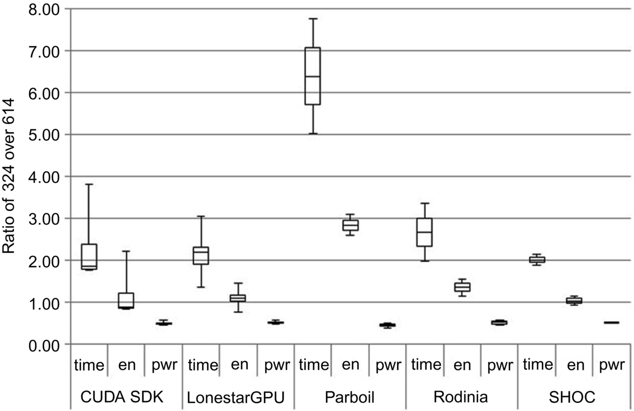
Fig. 9 shows the relative change in active runtime, energy, and power when switching from the default frequency setting to the 614 setting. Values above 1.0 indicate an increase over the default. In the figure, the horizontal line where the two boxes touch represents the median, the boxes above and below extend to the first and third quartiles, and the whiskers indicate the maximum and minimum for the studied programs from each benchmark suite.

The 614 configuration has a core speed that is about 15% lower than the default, so one might expect to see roughly a 15% increase in active runtime. However, only a couple of the benchmark medians (CUDA SDK and LonestarGPU) and a few individual programs slow down anywhere near 15%. This is because going from default to 614 only lowers the core frequency but not the memory frequency. Hence memory-bound programs show little to no change, including many codes in the Parboil, Rodinia, and SHOC suites. In contrast, most of the tested SDK programs are compute-bound. A few programs show a slight speedup, but many of those measurements are within the margin of error (i.e., the average variability among repeated measurements).
Switching to the 614 configuration affects the LonestarGPU suite the most. In fact, this suite includes both the worst increase and the best decrease in active runtime as well as the highest median increase. At first glance, this may appear surprising as LonestarGPU contains only programs with irregular memory accesses, which tend to be memory-bound, particularly on GPUs where they often result in uncoalesced memory accesses [11]. Hence lowering the core frequency while keeping the memory frequency constant should not affect the runtime much. However, irregular programs, by definition, exhibit data-dependent runtime behavior, which frequently leads to timing-dependent behavior. This means that, if a computation is waiting for a value, the time at which the value becomes available can have unforeseen effects on the runtime behavior of the program. As a consequence, small changes in timing—for example, due to lowering the core frequency—can have a large effect on the runtime. This is why the active runtime of some LonestarGPU programs changes by more than the clock frequency. Note that this effect can be positive or negative, which explains why LonestarGPU exhibits the widest range in runtime change and includes both the program that is helped the most and the program that is hurt the most by going to the 614 configuration.
Interestingly, going from the default to the 614 configuration results in a small beneficial effect on energy for most codes. Even though the programs tend to run longer, the amount of energy the GPU consumes decreases slightly in almost all cases except for LonestarGPU, where the energy consumption is mostly unaffected. Even in the worst cases, the energy does not increase by nearly as much as the active runtime.
This general decrease in energy is the result of a significant reduction in the power draw when switching to the 614 setting, which outweighs the increase in runtime on every program we studied. Even in the worst cases, the power decreases slightly or stays roughly constant. The median power decrease is between 3% and 10% depending on the benchmark suite. For memory-bound codes, lowering the switching activity in the underutilized core is expected to reduce power more than it increases the runtime. However, some of the compute-bound codes also experience a substantial power reduction. In fact, two of the compute-bound CUDA SDK programs experience a power reduction of over 15%, that is, more than the reduction in core frequency. We surmise that this is because, in addition to the frequency, the supply voltage is also reduced as is commonly done in DVFS [12]. Because power is proportional to the voltage squared, superlinear power reductions are possible [13].
NB from the CUDA SDK sees the greatest savings in power (22%) for the reasons just stated. It also has one of the largest increases in active runtime (15%) as it is highly compute bound, resulting in a middling decrease in energy (7%). Interestingly, just behind NB for decrease in power is the irregular MST code from the LonestarGPU suite. It has the highest increase in active runtime of all the programs across all the benchmarks (25%) and the third highest increase in energy (8%) and saves 16% in power. SHOC’s MF boasts the greatest savings in energy (14.3%) and one of the lowest increases in active runtime (1%). It saves 15% in power, making it the third best in terms of power reduction.
4.3.2 614 to 324
Fig. 10 is similar to Fig. 9 except it shows the relative change in active runtime, energy, and power when switching from the 614 to the 324 configuration. Note, however, that the two figures should not be compared directly as a number of programs did not yield sufficient power samples with the 324 configuration. Hence Fig. 10 is based on significantly fewer programs.
Switching from the 614 to the 324 configuration not only involves a 1.9-fold decrease in core frequency but, much more importantly, also an 8-fold decrease in memory frequency. The cumulative effect is an average increase in active runtime of over 110% across the studied programs. Except for some irregular programs, where the change in timing affects the load balance and the amount of parallelism (cf. the explanation in the previous section), all investigated programs are slowed down by at least a factor of 1.9 as expected.
Going from default to 614, two-thirds of the programs see a savings in energy, albeit small. In contrast, going from 614 to 324 increases the energy consumption of two-thirds of the programs, in one case by over 200%. Even in the best case, the energy savings do not exceed 30% and, on average, going from 614 to 324 results in an increase in energy. The reason for this change in behavior is the large slowdown in memory frequency when going to 324, which makes the programs more memory-bound, that is, the GPU cores end up idling more, thus wasting energy. The resulting increase in active runtime more than outweighs the decrease in power draw. In contrast, on the 614 configuration, the active runtime increases less than or roughly in proportion to the decrease in power draw, so the energy consumption decreases or stays roughly the same.
Looking at the individual codes, PTA from the LonestarGPU suite sees the smallest decrease in active runtime and the largest decrease in energy when going from 614 to 324, but because of the small drop in active runtime compared to the other programs, it also has one of the smallest savings in power. LBM from the Parboil suite sees the largest increase in active runtime (7.75×) and energy (2×).
According to Fig. 10, the Parboil suite experiences by far the largest increase in active runtime and energy. This is misleading, though, as only one of the Parboil programs (LBM) yielded usable results on the 324 configuration. In fact, the two LBM inputs used resulted in the two highest increases in runtime and energy out of all the programs we studied. This is a good example of how big an impact altering the memory frequency of the GPU can have on an already memory-bound code.
4.4 Input Sensitivity
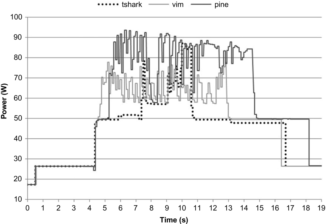
Fig. 11 shows how using different inputs affects the power profile of the irregular PTA code. Clearly, each tested input yields a rather distinct profile. For example, pine results in an over 15 W higher average power draw than vim, and tshark yields a profile in which the power ramps up after an initial spike, whereas the other two inputs result in more spikes and exhibit a slightly decreasing trend in power draw over time. Because a change in input can have such a drastic effect on the power profile of irregular programs, it may not be possible to use information from one type of input to accurately characterize the behavior for a different input. In fact, even the early behavior of a running program may not be indicative of its later behavior during the same run, as tshark illustrates. These potential problems need to be taken into account when making profile-based design decisions or implementing feedback-driven and online code optimizations.
4.5 Source-Code Optimizations
In this section, we again look at the irregular memory-bound BH code from the LonestarGPU suite and compare it to the regular compute-bound NB code. We modified these two programs in a way that makes it possible to individually enable or disable specific source-code transformations. We study the effect of the these code optimizations on the runtime, energy, and power for different core and memory frequencies, with and without using error correcting codes (ECC) in main memory, and with single and double precision. As in the Core and Memory Frequency Scaling section, we use the default, 614, and 324 frequency settings (see the aforementioned section for details). To these settings we add the “ECC” configuration, which combines ECC protection with the default clock frequency. On the K20c, enabling ECC has the effect of increasing the number of memory accesses a particular program makes without increasing the amount of computation done in software. All other tested configurations have ECC disabled. We also add the “double” configuration. By default, the evaluated programs use single-precision floating-point arithmetic, but we also wrote double-precision versions for comparison. Since CUDA-enabled GPUs require two registers to hold a double value and can store only half as many doubles as floats in shared memory, the “double” configuration has to run with fewer threads than the single-precision codes. Because of this, the single- and double-precision configurations used in this chapter are not directly comparable.
These experiments were conducted on three inputs varying both the number of bodies and the number of time steps. We found the differences in behavior between the inputs to be slight, so the results shown here are from just one set of inputs: 100,000 bodies with 100 time steps for NB, and 1 million bodies with 1 time step for BH.
For NB, we chose the following six code optimizations:
(1) unroll “u” uses a pragma to request unrolling of the innermost loop(s). Unrolling often allows the compiler to schedule instructions better and to eliminate redundancies, thus improving performance.
(2) shmem “s” employs blocking; that is, it preloads chunks of data into the shared memory, operates exclusively on this data, then moves on to the next chunk. This greatly reduces the number of global memory accesses.
(3) peel “p” separates the innermost loop of the force calculation into two consecutive loops, one of which has a known iteration count and can therefore presumably be better optimized by the compiler. The second loop performs the few remaining iterations.
(4) const “c” copies immutable kernel parameters once into the GPU’s constant memory rather than passing them every time a kernel is called; that is, it lowers the calling overhead.
(5) rsqrt “r” uses the CUDA intrinsic “rsqrtf()” to quickly compute one over square root instead of using the slower but slightly more precise “1.0f/sqrtf()” expression.
(6) ftz “f” is a compiler flag that allows the GPU to flush denormal numbers to 0 when executing floating-point operations, which results in faster computations. While strictly speaking it is not a code optimization, the same effect can be achieved by using appropriate intrinsic functions in the source code.
For BH, we selected the following six code optimizations:
(1) vola “v” strategically copies some volatile variables into nonvolatile variables and uses those in code regions where it is known (due to lockstep execution of threads in a warp) that no other thread can have updated the value. This optimization serves to reduce memory accesses.
(2) ftz “f” is identical to the corresponding NB optimization.
(3) rsqrt “r” is also identical to its NB counterpart.
(4) sort “s” approximately sorts the bodies by spatial distance to minimize the tree prefix that needs to be traversed during the force calculation.
(5) warp “w” switches from a thread-based to a warp-based implementation that is much more efficient because it does not suffer from branch divergence and uses less memory because it records certain information on a per-warp instead of a per-thread basis.
(6) vote “V” employs thread voting instead of a shared memory-based code sequence to perform 32-element reductions.
Because we can individually enable or disable each optimization, there are 64 possible combinations of the 6 optimizations. Consequently, we evaluate 64 versions for both the NB and BH codes.
4.5.1 None vs all optimizations
Table 1 shows the measured active runtime and energy consumption as well as the average power draw of the five evaluated configurations for the second inputs when none and all of the optimizations are enabled.
Table 1
Active Runtime (s), Energy (J), and Power (W) With the Second Input When None and All of the Optimizations Are Enabled
| Default | 614 | 324 | ECC | Double | ||||||||||||
| Runtime | Energy | Power | Runtime | Energy | Power | Runtime | Energy | Power | Runtime | Energy | Power | Runtime | Energy | Power | ||
| NB | None | 63.88 | 7002 | 109.6 | 73.44 | 6902 | 94.0 | 135.85 | 6250 | 46.0 | 64.08 | 7078 | 110.5 | 154.64 | 17, 857 | 115.5 |
| All | 12.10 | 1828 | 151.1 | 13.88 | 1745 | 125.7 | 26.97 | 1580 | 58.6 | 12.16 | 1840 | 151.4 | 47.33 | 7137 | 150.8 | |
| BH | None | 209.09 | 26, 266 | 125.6 | 237.18 | 26, 255 | 110.7 | 739.92 | 34, 868 | 47.1 | 211.81 | 27, 301 | 128.9 | 304.25 | 37, 897 | 124.6 |
| All | 16.15 | 1966 | 121.7 | 18.19 | 1952 | 107.3 | 40.72 | 2142 | 52.6 | 18.33 | 2277 | 124.2 | 26.18 | 3328 | 127.1 | |
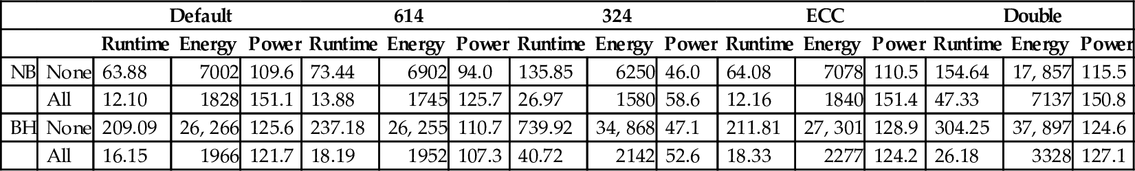
Our first observation is that code optimizations can have a large impact not only on active runtime but also on energy and power. On NB, the energy consumption improves 2.5- to 4-fold due to the optimizations, and the performance improves 3.3- to 5.3-fold. At the same time, the power increases by up to 30% because the hardware is being used more effectively. On BH, the energy improves 11- to 16-fold and the performance 11.5- to 18-fold while the power increases by 10%. Clearly, code optimizations can drastically lower the active runtime and the energy, but tend to increase power.
The improvements are substantially lower on NB than on BH. We believe there are two main reasons for this difference. First, NB is a much simpler and shorter code, making it easier to implement efficiently without having to resort to sophisticated optimizations. Second, NB is a regular code with few data dependencies, enabling the compiler to generate quite efficient code even in the base case. As a consequence, the additional code optimizations we analyzed provide less benefit.
Focusing on the default configuration, we find that the optimizations help the active runtime of NB much more than the energy consumption, which is why the power increases greatly. On BH, the situation is different. Here, the optimizations reduce the energy consumption a little more than the active runtime, resulting in a slight decrease in power draw.
Comparing the default and the 614 configurations, we find that the 15% drop in core speed yields a 15% active runtime increase on NB, as previously discussed. The active runtime of BH increases only by 13%, because the memory accesses are not slowed down. Hence the drop in power draw is lower for BH than for NB. The 614 configuration consumes a little less energy than the default configuration. The reduction is within the margin of error for BH, but the 5% drop with all optimizations enabled on NB is significant. Overall, the 614 configuration primarily serves to lower the power draw. Because of a concomitant increase in active runtime, it does not affect the energy much. The benefit of all the various optimizations is fairly similar for the default and 614 configurations.
The 324 configuration behaves quite differently because it not only reduces the core frequency by a factor of 2 but also lowers the memory frequency by a factor of 8 relative to the 614 configuration. NB’s increase in active runtime is in line with the twofold drop in core frequency because it is compute-bound, whereas BH’s increase in active runtime is much larger due to its greater dependence on memory speed. As a consequence, there is a decrease in energy consumption on NB but a substantial increase on BH when comparing the 324 to the 614 configuration. Because the 324 configuration affects the active runtime much more than the energy, it results in a large decrease in power draw. Reducing power is the primary strength of the 324 configuration, which is otherwise not very useful and can greatly increase the energy consumption of memory-bound codes. Nevertheless, the code optimizations are just as effective on it as they are on the other configurations. In fact, on BH, they are more effective when using the 324 configuration because the optimizations eliminate some of the now extremely costly memory accesses.
Looking at the ECC configuration, we find that the energy, active runtime, and power numbers are almost identical to the default for NB. Since NB has excellent locality, which translates into many cache/shared-memory hits and good coalescing, even the version without our optimizations performs relatively few main memory accesses, which is why it is hardly affected by ECC. BH has less locality and accesses memory more frequently, which explains why it is affected more. Its active runtime and energy become 13% and 16% worse, respectively, when ECC is turned on and all optimizations are used. However, the active runtime and energy are only 1% and 4% worse with ECC when none of the optimizations are enabled. We believe the reason for this difference is that the optimizations improve the computation more than the memory accesses, thus making the optimized code, relatively speaking, more memory-bound.
Comparing the double configuration to the default, we observe that the active runtime and energy are 1.5–3.9 times worse, but the power is almost unchanged. Clearly, the double-precision code is substantially slower. While still highly effective (a factor of 2.5–11.6 improvement), the benefit of the code optimizations is lower for the double configuration. This is probably because the double-precision code is more memory-bound than the single-precision code, and as previously mentioned the optimizations improve the computation more than the memory accesses.
4.5.2 Effectiveness of optimizations
Fig. 12A and B shows the range of the effect of each optimization on the active runtime and the energy. The 64 versions of each program contain 32 instances that do not and 32 that do include any given optimization. The presented data show the maximum (top whisker), the minimum (bottom whisker), and the median (line between the two boxes) change when adding a specific optimization to the 32 versions that do not already include it. The boxes represent the first and third quartiles, respectively. Points below 1.0 indicate a slowdown or increase in energy consumption. It is clear from these figures that the effect of an optimization can depend greatly on what other optimizations are present.

The most effective optimization on NB is rsqrt. Using this special intrinsic improves the energy and particularly the active runtime because it targets the slowest and most complex operation in the innermost loop. Since rsqrt helps the active runtime more than the energy, it increases the power substantially. The other very effective optimization is shmem, that is, to use tiling in shared memory. It, too, improves the active runtime more than the energy, leading to an increase in power.
The impact of the remaining four optimizations is much smaller. ftz helps both energy and active runtime as it speeds up the processing of the many floating-point instructions. It is largely power-neutral because it improves energy and active runtime about equally. Except with the double configuration, unroll helps active runtime a little and energy a lot, thus lowering the power quite a bit. We are not sure why unrolling helps energy more. const hurts the energy consumption and the active runtime, but it is close to the margin of error. After all, this optimization only affects the infrequent kernel launches. peel hurts performance and energy, except in the double-precision code, but does not change the power much. Clearly, there are optimizations that help active runtime more (e.g., rsqrt) while others help energy more (e.g., unroll). Some optimizations help both active runtime and energy equally (e.g., ftz).
Most of the optimization benefits are quite similar across the different configurations. Notable 324 exceptions are peel, which hurts significantly more than in the other configurations, and ftz and rsqrt, which are more effective on 324. shmem and unroll are also more effective. Interestingly, the double configuration exhibits almost exactly the opposite behavior. peel is more effective on it than on the other configurations, whereas ftz, rsqrt, shmem, and unroll are substantially less effective.
The findings for BH are similar. There are also two optimizations that help a great deal. warp, the most effective optimization, improves energy a little less than active runtime, thus increasing the power draw. sort, the second most effective optimization, helps energy a little more than active runtime. vola and rsqrt also help both aspects but are much less effective and power-neutral. We are surprised by the effectiveness of vola. Apparently, it manages to reduce memory accesses significantly and therefore makes BH less memory-bound. vote helps energy substantially more than active runtime. Hence this optimization is particularly useful for reducing power. Interestingly, on some configurations, it hurts both energy and active runtime, on others only active runtime; yet on others, it helps both aspects. ftz is within the margin of error but seems to help a little. The reason why both rsqrt and ftz are much less effective on BH than on NB is because BH executes many integer instructions, which do not benefit from these optimizations.
Investigating the individual configurations, we again find that there is no significant difference in optimization effectiveness between default and 614 as well as between default and ECC on NB. For 324 on NB, const is unchanged, peel is less effective, and the other optimizations are more effective than with the default configuration. On BH, warp and vola are much more effective with the 324 configuration. This is because both optimizations reduce the number of memory accesses. For ECC on BH, vote is less effective, but the other optimizations are just as effective as they are with the default configuration.
Once again, the double configuration behaves quite differently. Most notably, warp is much less effective and vola somewhat less. However, rsqrt and especially vote are more effective. Note that in the double-precision code, the rsqrtf() intrinsic is followed by two Newton-Raphson steps to obtain double precision, which is apparently more efficient, both in terms of active runtime and energy, than performing a double-precision square root and division. Thread voting helps because it frees up shared memory that can then be used for other purposes. For NB, the double configuration results in peel being much more effective and all other optimizations except const being much less effective than using the default configuration. In particular, rsqrt and shmem are substantially less effective, the former because of the Newton-Raphson overhead, which is substantial in the tight inner loop of NB, and the latter because only half as many double values fit into the shared memory. Overall, the power is not much different for the double configuration with the exception of unroll, which does not lower the power draw in the double-precision code.
These results illustrate that the effect of a particular optimization is not always constant but can change depending on the regular or irregular nature of the code, the core and memory frequencies, the chosen floating-point precision, and the presence or absence of other source-code optimizations.
4.5.3 Lowest and highest settings
Fig. 13 displays the sets of optimizations that result in the highest and lowest active runtime and energy. In each case, a six-character string shows which optimizations are present (see the beginning of this section for which letter represents which optimization). The characters are always listed in the same order. An underscore indicates the absence of the corresponding optimization.

Interestingly, the worst performance and the highest energy are obtained when some optimizations are enabled, showing that it is possible for “optimizations” to hurt rather than help. In the worst case, which is NB 324, the energy consumption increases more than threefold when going from none of the optimizations to enabling peel. For all tested configurations, the best performance and the lowest energy consumption on BH are always obtained when all optimizations are enabled. This is also mostly the case for NB. Comparing the highest to the lowest values, we find that the worst and best configurations differ by over a factor of 12 (energy) and 14 (active runtime) on NB and by over a factor of 29 (energy) and 34 (active runtime) on BH. This highlights how large an effect code transformations can have on performance and energy consumption. The effect on the power is modest in comparison. It changes by up to 23% on BH and up to 60% on NB.
Looking at individual optimizations, we find that, except for the worst case with the double configuration, peel is always included in the best and the worst settings in NB. Clearly, peel is bad when used by itself or in combination with the const optimization. However, peel becomes beneficial when grouped with some other optimizations, demonstrating that the effect of an optimization cannot always be assessed in isolation but may depend on the context. To reach the lowest power on NB, unroll, peel, and const need to be enabled together.
In the case of BH, we find sort and vote to dominate the worst active runtime and energy settings. sort in the absence of warp does not help anything. vote generally hurts energy and often active runtime (cf. Section 3.3). Surprisingly, ftz is often included in the worst performance setting for BH. We expected ftz to never increase the active runtime. However, ftz also appears in all the best settings, showing that it does help in the presence of other optimizations.
Additionally, the best and worst settings are similar across the different configurations, illustrating that optimizations tend to behave consistently with respect to each other.
4.5.4 Energy efficiency vs performance
Table 2 shows the largest impact that adding a single optimization makes. We consider four scenarios, maximally hurting both active runtime and energy, hurting active runtime but improving energy, improving active runtime but hurting energy, and improving both active runtime and energy.
Table 2
Base Setting and Added Optimization That Yields the Most Significant Positive/Negative Impact
| Default | 614 | 324 | ECC | Double | ||||||||||||
| Setting & Opt | Impr. Factor | Setting & Opt | Impr. Factor | Setting & Opt | Impr. Factor | Setting & Opt | Impr. Factor | Setting & Opt | Impr. Factor | |||||||
| Time | Ener. | Time | Ener. | Time | Ener. | Time | Ener. | Time | Ener. | |||||||
| NB | rt+en+ | ___ & peel | 0.63 | 0.47 | ___ & peel | 0.63 | 0.47 | ___ & peel | 0.34 | 0.32 | ___ & peel | 0.63 | 0.46 | __per&unrol | 0.86 | 0.91 |
| rt+en− | __pc f&unrol | 0.86 | 1.25 | __pc f & unrol | 0.86 | 1.24 | __pc_f&unrol | 0.97 | 1.26 | _pc_f&unrol | 0.86 | 1.28 | __us_rf&const | 1.00 | 1.00 | |
| rt− en+ | _sp_rf & const | 1.01 | 1.00 | _sp_rf & const | 1.01 | 1.00 | _sp_rf & const | 1.00 | 0.99 | _sp_rf&const | 1.01 | 1.00 | _us_cr&peel | 1.00 | 0.97 | |
| rt− en− | __P___ & rsqrt | 2.97 | 3.65 | __P___ & rsqrt | 2.97 | 3.69 | __pc__ & rsqrt | 5.33 | 5.29 | __P___ &rsqrt | 2.98 | 3.74 | __P___ &rsqrt | 2.27 | 1.90 | |
| BH | rt+en+ | _frs__ & vote | 0.16 | 0.18 | _frs__ & vote | 0.16 | 0.18 | _frs__ & vote | 0.15 | 0.16 | _frs__ & vote | 0.15 | 0.17 | _frs__ & vote | 0.22 | 0.24 |
| rt+en− | ___wV & vola | 0.99 | 1.04 | ___wV & vola | 1.00 | 1.05 | v_rs__ & ftz | 1.00 | 1.01 | ___wV & vola | 0.99 | 1.04 | ____ & vote | 0.96 | 1.07 | |
| rt− en+ | n/a | n/a | n/a | v__swV & ftz | 1.00 | 1.00 | ___w & ftz | 1.00 | 1.00 | ___s__ & ftz | 1.00 | 1.00 | ____V & ftz | 1.00 | 1.00 | |
| rt− en− | __frs_V & warp | 19.06 | 17.04 | _frs_V & warp | 19.28 | 17.48 | _frs_V & warp | 27.47 | 23.99 | frs_V & warp | 18.31 | 16.64 | frs_V & warp | 13.03 | 11.40 | |

Notes: +, an increase; −, a decrease; en, energy; rt, active runtime.
With one exception, every configuration has examples of all four scenarios. The examples of decreasing the active runtime while increasing the energy consumption are within the margin of error and therefore probably not meaningful. However, the other three scenarios have significant examples. Excluding the double configuration for the moment, enabling just the peel optimization on NB increases the energy consumption by more than a factor of 2 and the active runtime by nearly as much (as noted in the previous section). Clearly, this “optimization” is a very bad choice by itself. However, adding rsqrt to the peel optimization improves the active runtime and energy by a factor of 3–5, making it the most effective addition of an optimization we have observed. Perhaps the most interesting case is adding unroll to peel, const, and ftz. It lowers the energy consumption by about 25% even though it increases the active runtime substantially. This example shows that performance and energy optimization are not always the same thing.
BH has similar examples. Adding vote to ftz, rsqrt, and sort greatly increases the active runtime and the energy consumption, making it the worst example of adding an optimization. In contrast, adding warp to ftz, rsqrt, and sort greatly reduces both active runtime and energy, making it the most effective addition of a single optimization we have observed. Again, decreasing the active runtime while increasing the energy is within the margin of error (or no such case exists). Finally, there are several examples of lowering the energy by a few percent while increasing the active runtime marginally. Although not as pronounced as with NB, these examples again show that there are cases that only help energy but not active runtime.
The base settings and the optimizations added that result in significant changes in energy and active runtime are consistent across the five configurations. Only the double configuration on NB differs substantially. However, even in this case, the effects of the optimizations are large. In fact, this configuration exhibits the most pronounced example of adding an optimization that lowers the active runtime (albeit within the margin of error) while increasing the energy consumption (by 3%).
4.5.5 Most biased optimizations
This section studies optimizations where the difference between how much they improve energy versus active runtime is maximal. Table 3 provides the results for the different configurations.
Table 3
Base Setting and Added Optimization That Yields the Most Biased Impact on Energy Over Active Runtime and Vice Versa on the Second Input
| Default | 614 | 324 | ECC | Double | ||||||||||||
| Setting & Opt | Impr. Factor | Setting & Opt | Impr. Factor | Setting & Opt | Impr. Factor | Setting & Opt | Impr. Factor | Setting & Opt | Impr. Factor | |||||||
| Time | Ener. | Time | Ener. | Time | Ener. | Time | Ener. | Time | Ener. | |||||||
| NB | max en over rt | __pc__ & unrol | 1.19 | 1.82 | __pc__ & unrol | 1.19 | 1.80 | __pc_f & unrol | 0.97 | 1.26 | __pc__& unrol | 1.19 | 1.86 | _sp_r_ & ftz | 1.01 | 1.02 |
| max rt ove ren | uspc__ & rsqrt | 3.65 | 2.53 | uspc__ & rsqrt | 3.65 | 2.61 | uspc__ & rsqrt | 3.50 | 2.66 | uspc__ & rsqrt | 3.66 | 2.52 | __p___ & rsqrt | 2.27 | 1.90 | |
| BH | max en over rt | ___wV & vola | 0.99 | 1.04 | __rs__ & warp | 1.11 | 1.18 | ___wV & sort | 3.01 | 3.16 | _frs__ & warp | 1.10 | 1.16 | ____ & vote | 0.96 | 1.07 |
| max rt over en | ____V & warp | 4.36 | 3.81 | _v_rs__V & warp | 18.13 | 16.13 | __f___V & warp | 7.56 | 6.25 | ____V & warp | 4.99 | 4.29 | vfrs_V & warp | 11.59 | 10.13 | |

On NB, we find that adding unroll to peel and const improves energy by 18–56% more than active runtime except for double, where there is no strong example. In contrast, adding rsqrt to unroll, shmem, peel, and const improves active runtime by 31–46% more than energy, again with the exception of the double configuration, where the same optimization but on a different base setting yields 20% more benefit in active runtime than in energy.
On BH, there is no consistent setting or optimization that yields the highest benefit in energy over active runtime. Nevertheless, some code optimizations help energy between 5% and 18% more than active runtime. The best optimization for helping active runtime more than energy is warp, but the base setting differs for the different configurations. It improves active runtime between 6% and 21% more than energy.
These results highlight that optimizations do not necessarily affect active runtime and energy in the same way. Rather, some source-code optimizations tend to improve one aspect substantially more than another.
5 Summary
Understanding performance, energy, and power on GPUs is becoming more and more important as GPU-based accelerators are quickly spreading to every corner of computing, including handheld devices and supercomputers where reducing power and energy while maintaining performance is highly desirable and a key trade-off that has to be considered when designing new systems.
In this chapter, we show that the power profiles of regular codes are often similar to the expected “rectangular” power profile but that irregular codes often are not. Because of this, assumptions on the energy consumption of an irregular program based on that program’s power profile from an earlier run may not be accurate.
We also made the following observations. Because of their more efficient use of the hardware, regular compute-bound codes tend to draw substantially more power than irregular memory-bound codes. Changing the implementation of programs can be a very effective tool to lower the power draw and active runtime, and thus the energy consumption. Lowering the GPU frequency is a good power-saving strategy but not useful as an energy-saving strategy, and doing so is bad for performance, as expected. Switching from single- to double-precision arithmetic has little effect on the power but drastically increases both the active runtime and the energy consumption of the GPU.
Using ECC with even slightly memory-bound programs not only results in a slowdown but also in a concomitant increase in energy consumption. ECC’s cost is entirely dependent on how many main-memory accesses a program makes, so code transformations that reduce the number of (main) memory accesses are especially useful when ECC is active. Compute-bound codes are mostly unaffected by ECC in terms of performance, power draw, and energy consumption.
Source-code optimizations tend to increase the power draw and can have a large impact on energy. The effect of an optimization cannot always be assessed in isolation but may depend on the presence of other optimizations. Also, source-code optimizations do not necessarily affect active runtime and energy in the same way. Some optimizations hurt when used by themselves but can become beneficial when grouped with other optimizations, so optimizations should not be judged in isolation.
We identified several examples where code optimizations lower the energy while increasing the active runtime, showing that there are optimizations that help energy but not active runtime. In one case, the improvement in energy is 56% higher than the improvement in active runtime. In another case, the active runtime improvement is 46% higher than the energy improvement.
Our results demonstrate that programmers can optimize their source code for energy (or power), that such optimizations may be different from optimizations for performance, and that optimizations can make a large difference. Clearly, source-code optimizations have the potential to play an important role in making accelerators more energy-efficient.
Our results show that there are several software-based methods for controlling power draw and energy consumption, some of which certainly increase the active runtime, but others help active runtime. These methods include changing the GPU’s clock frequency, altering the arithmetic precision, turning ECC on or off, utilizing a different algorithm, and employing source-code optimizations. Some of these methods are directly accessible to the end user, whereas others need to be implemented by the programmer.
We make the following recommendations for anyone interested in performing power and energy studies on GPUs:
(1) Use program inputs that result in long runtimes to obtain enough power samples to accurately analyze the energy and power behavior. However, avoid poor implementations that run slowly.
(2) Measure a broad spectrum of codes, including memory- and compute-bound programs as well as regular and irregular codes since they exhibit different behaviors.
(3) As none of the studied benchmark suites include all of these types of applications, use programs from different suites for conducting power and energy studies.
(4) Run irregular codes with multiple inputs that exercise different behaviors.
(5) Repeat experiments at various frequency and ECC settings if desired as the findings might change.
Portions of this chapter are based on published work that contains more detailed information [14–16].
Appendix
(1) LonestarGPU. The LonestarGPU suite is a collection of commonly used real-world applications that exhibit irregular behavior.
(a) Barnes-Hut n-body simulation (BH): An algorithm that quickly approximates the forces between a set of bodies in lieu of performing precise force calculations.
(b) Breadth-first search (L-BFS): Computes the level of each node from a source node in an unweighted graph using a topology-driven approach. In addition to the standard BFS implementation (topology-driven, one node per thread), we also study the atomic variation (topology-driven, one node per thread that uses atomics) and the wla variation (topology-driven, one flag per node, one node per thread). The wlw variation (data-driven, one
Table 4
Program Names, Number of Global Kernels (#K), and Inputs
| Program | #K | Inputs | Program | #K | Inputs |
| EIP | 2 | None | SGEMM | 1 | “small” benchmark input |
| EP | 2 | None | STEN | 1 | “small” benchmark input |
| NB | 1 | 100k, 250k, and lm bodies | TPACF | 1 | “small” benchmark input |
| SC | 3 | 2∧26 elements | BP | 2 | 2∧17 elements |
| BH | 9 | Bodies-timesteps; 10k-10k, 100k-10, lm-1 | R-BFS | 2 | Random graphs; 100k and lm nodes |
| L-BFS | 5 | Roadmaps of Great Lakes Region (2.7m nodes, 7m edges), Western USA (6m nodes, 15m edges), and entire USA (24m nodes, 58m edges) | GE | 2 | 2048 × 2048 matrix |
| DMR | 4 | 250k, lm, and 5m node mesh files | MUM | 3 | 100 and 25 bp |
| MST | 7 | Roadmaps of Great Lakes Region (2.7m nodes, 7m edges), Western USA (6m nodes, 15m edges), and entire USA (24m nodes, 58m edges) | NN | 1 | 42k data points |
| PTA | 40 | vim (small), pine (medium), tshark (large) | NW | 2 | 4096 and 16,384 items |
| SSSP | 2 | Roadmaps of Great Lakes Region (2.7m nodes, 7m edges), Western USA (6m nodes, 15m edges), and entire USA (24m nodes, 58m edges) | PF | 1 | Row length-column length-pyramid height; 100k-100-20, 200k-200-40 |
| NSP | 3 | Clauses-literals-literals per clause; 16,800-4000-3, 42k-10k-3, 42k-10k-5 | S-BFS | 9 | Default benchmark input |
| P-BFS | 3 | Roadmap of the San Francisco Bay Area (321k nodes, 800k edges) | FFT | 2 | Default benchmark input |
| CUTCP | 1 | watbox.sll00.pqr | MF | 20 | Default benchmark input |
| HISTO | 4 | Image file whose parameters “– are 20-4” according to documentation | MD | 1 | Default benchmark input |
| LBM | 1 | 3000 and 100 timestep inputs | QTC | 6 | Default benchmark input |
| MRIQ | 2 | 64 × 64 × 64 matrix | ST | 5 | Default benchmark input |
| SAD | 3 | Default input | S2D | 1 | Default benchmark input |

node per thread) and the wlc variation (data-driven, one edge-per-thread version using Merrill’s strategy [17]) were not used because they reduced the active runtime to the point that insufficient power samples could be recorded even with the largest available input.
(c) Delaunay mesh refinement (DMR): This implementation of the algorithm described by Kulkarni et al. [18] produces a guaranteed quality 2D Delaunay mesh, which is a Delaunay triangulation with the additional constraint that no angle in the mesh be less than 30 degrees.
(d) Minimum spanning tree (MST): This benchmark computes a minimum spanning tree in a weighted undirected graph using Boruvka’s algorithm and is implemented by successive edge relaxations of the minimum weight edges.
(e) Points to analysis (PTA): Given a set of points-to-constraints, this code computes the points-to information for each pointer in a flow-insensitive, context-insensitive manner implemented in a topology-driven way.
(f) Single-source shortest paths (SSSP): Computes the shortest path from a source node to all nodes in a directed graph with nonnegative edge weights by using a modified Bellman-Ford algorithm. In addition to the standard SSSP implementation (topology-driven, one node per thread), we also used the wln variation (data-driven, one node per thread) and the wlc variation (data-driven, one edge per thread using Merrill’s strategy adapted to SSSP).
(g) Survey propagation (NSP): A heuristic SAT-solver based on Bayesian inference. The algorithm represents the Boolean formula as a factor graph, which is a bipartite graph with variables on one side and clauses on the other.
(2) Parboil. Parboil is a set of applications used to study the performance of throughput-computing architectures and compilers.
(a) Breadth-first search (P-BFS): Computes the shortest-path cost from a single source to every other reachable node in a graph of uniform edge weights.
(b) Distance-cutoff Coulombic potential (CUTCP): Computes the short-range component of the Coulombic potential at each grid point over a 3D grid containing point charges representing an explicit-water biomolecular model.
(c) Saturating histogram (HISTO): Computes a 2D saturating histogram with a maximum bin count of 255.
(d) Lattice-Boltzmann method fluid dynamics (LBM): A fluid dynamics simulation of an enclosed, lid-driven cavity using the LBM.
(e) Magnetic resonance imaging—Q (MRIQ): Computes a matrix Q, representing the scanner configuration for calibration, used in 3D magnetic resonance image reconstruction algorithms in non-Cartesian space.
(f) Sum of absolute differences (SAD): SAD kernel, used in MPEG video encoders.
(g) General matrix multiply (SGEMM): A register-tiled matrix-matrix multiplication, with default column-major layout on matrix A and C, but with B transposed.
(h) 3D stencil operation (STEN): An iterative Jacobi stencil operation on a regular 3D grid.
(i) Two-point angular correlation function (TPACF): Statistical analysis of the distribution of astronomical bodies.
(3) Rodinia. Rodinia is designed for heterogeneous computing infrastructures with OpenMP, OpenCL, and CUDA implementations. Our study uses the following CUDA codes.
(a) Back propagation (BP): ML algorithm that trains the weights of connecting nodes on a layered neural network.
(b) Breadth-first search (R-BFS): Another GPU implementation of the BFS algorithm, which traverses all the connected components in a graph.
(c) Gaussian elimination (GE): Computes results row by row, solving for all of the variables in a linear system.
(d) MUMmerGPU (MUM): A local sequence alignment program that concurrently aligns multiple query sequences against a single reference sequence stored as a suffix tree.
(e) Nearest neighbor (NN): Finds the k-nearest neighbors in an unstructured data set.
(f) Needleman-Wunsch (NW): A nonlinear global optimization method for DNA sequence alignment.
(g) Pathfinder (PF): Uses dynamic programming to find a path on a 2D grid with the smallest accumulated weights, where each step of the path moves straight or diagonally.
(4) SHOC. The Scalable HeterOgeneous Computing benchmark suite is a collection of programs that are designed to test the performance of heterogeneous systems with multicore processors, graphics processors, reconfigurable processors, and so on.
(a) Breadth-first search (S-BFS): Measures the runtime of BFS on an undirected random k-way graph.
(b) Fast Fourier transform (FFT): Measures the speed of a single- and double-precision fast Fourier transform that computes the discrete Fourier transform and its inverse.
(c) MaxFlops (MF): Measures the maximum throughput for combinations of different floating-point operations.
(d) Molecular dynamics (MD): Measures the performance of an n-body computation (the Lennard-Jones potential from MD). The test problem is n atoms distributed at random over a 3D domain.
(e) Quality threshold clustering (QTC): Measures the performance of an algorithm designed to be an alternative method for data partitioning.
(f) Sort (ST): Measures the performance of a Radix Sort on unsigned integer key/value pairs.
(g) Stencil2D (S2D): Measures the performance of a 2D, nine-point single-precision stencil computation.
(5) CUDA-SDK. The NVIDIA GPU Computing SDK includes dozens of sample codes. We use the following programs in our study.
(a) MC_EstimatePiInlineP (EIP): Monte Carlo simulation for the estimation of pi using a Pseudo-Random Number Generator (PRNG). The inline implementation allows use inside GPU functions/kernels as well as in the host code.
(b) MC_EstimatePiP (EP): Monte Carlo simulation for the estimation of pi using a PRNG. This implementation generates batches of random numbers.
(c) n-body (NB): All-pairs n-body simulation.
(d) Scan (SC): Demonstrates an efficient implementation of a parallel prefix sum, also known as “scan.”