
MPC
An effective floating-point compression algorithm for GPUsa
A. Yang; J. Coplin; H. Mukka; F. Hesaaraki; M. Burtscher Texas State University, San Marcos, TX, United States
Abstract
Because of their high peak performance and energy efficiency, massively parallel accelerators such as graphics processing units (GPUs) are quickly spreading in high-performance computing, where large amounts of floating-point data are processed, transferred, and stored. Such environments can greatly benefit from data compression if it is done quickly enough. Unfortunately, most conventional compression algorithms are unsuitable for highly parallel execution. In fact, how to design good compression algorithms for massively parallel hardware still is not fully understood. To remedy this situation, we studied millions of lossless compression algorithms for single- and double-precision floating-point values built exclusively from easily parallelizable components. We analyzed the best of these algorithms, explained why they compress well, and derived the Massively Parallel Compression algorithm from them. This algorithm requires little internal state, achieves heretofore unreached compression ratios (CRs) on several data sets, and roughly matches the best CPU-based algorithms in CR while outperforming them by one to two orders of magnitude in throughput and energy efficiency.
Keywords
Lossless data compression; Floating-point compression; Algorithm design; GPUs
Acknowledgments
This work was supported by the US National Science Foundation under Grants 1141022, 1217231, 1406304, and 1438963, a REP grant from Texas State University, and grants and gifts from NVIDIA Corporation. The authors acknowledge the Texas Advanced Computing Center for providing some of the HPC resources used in this study.
1 Introduction
High-performance computing (HPC) applications often process and transfer large amounts of floating-point data. For example, many simulations exchange data between compute nodes and with mass-storage devices after every time step. Most HPC programs retrieve and store large data sets, some of which may have to be sent to other locations for additional processing, analysis, or visualization. Moreover, scientific programs often save checkpoints at regular intervals.
Compression can reduce the amount of data that needs to be transmitted and/or stored. However, if the overhead lowers the effective throughput, compression will not be used in the performance-centric HPC domain. Hence the challenge is to maximize the compression ratio (CR) while meeting or exceeding the available transfer bandwidth. In other words, the compression and decompression have to be done in real time. Furthermore, the compression should be lossless and single pass. Intermediate program results that are exchanged between compute nodes, for example, generally cannot be lossy. A single-pass algorithm is needed so that the data can be compressed and decompressed in a streaming fashion as they are being generated and consumed, respectively.
Some compression algorithms are asymmetric, meaning that compression takes much longer than decompression. This is useful in situations where data are compressed once and decompressed many times. However, this is not the case for checkpoints, which are almost never read, nor for intermediate program results that are compressed to boost the transmission speed between compute nodes, between accelerators and hosts, or between compute nodes and storage devices. Thus we focus on symmetric algorithms in this chapter.
Massively parallel compute graphics processing units (GPUs) are quickly spreading in HPC environments to accelerate calculations as GPUs not only provide much higher peak performance than multicore CPUs but also are more cost- and energy-efficient. However, utilizing GPUs for data compression is difficult because compression algorithms typically compress data based on information from previously processed words. This makes compression and decompression data-dependent operations that are difficult to parallelize. Thus most of the relatively few parallel compression approaches from the literature simply break the data up into chunks that are compressed independently using a serial algorithm. However, this technique is not suitable for massively parallel hardware. First, the data would have to be broken up into hundreds of thousands of small chunks, at least one per thread, thus possibly losing much of the history needed to compress the data well. Second and more importantly, well-performing serial compression algorithms generally require a large amount of internal state (e.g., predictor tables or dictionaries), making it infeasible to run tens of thousands of them in parallel. As a consequence, the research community does not yet possess a good understanding of how to design effective compression algorithms for massively parallel machines.
At a high level, most data compression algorithms comprise two main steps, a data model and a coder. Roughly speaking, the goal of the model is to predict the data. The residual (i.e., the difference) between each actual value and its predicted value will be close to zero if the model is accurate for the given data. This residual sequence of values is then compressed with the coder by mapping the residuals in such a way that frequently encountered values or patterns produce shorter output than infrequently encountered data. The reverse operations are performed to decompress the data. For instance, an inverse model takes the residual sequence as input and regenerates the original values as output.
To systematically search for effective and massive parallelism-friendly compression algorithms, we synthesized a large number of compressors and their corresponding decompressors using the following approach. We started with a detailed study of previously proposed floating-point compression algorithms [2–14]. Short overviews of these algorithms as well as additional related work are available elsewhere [1]. We then broke each algorithm down into their constituent parts, rejected all parts that could not be parallelized well, and generalized the remaining parts as much as possible. This yielded a number of algorithmic components for building data models and coders. We then implemented each component using a common interface, that is, each component can be given a block of data as input, which it transforms into an output block of data. This makes it possible to chain the components, allowing us to generate a vast number of compression-algorithm candidates from a given set of components. Note that each component comes with an inverse that performs the opposite transformation. Thus, for any chain of components, which represents a compression algorithm, we can synthesize the matching decompressor. Fig. 1 illustrates this approach on the example of the four components named LNV6s, BIT, LNV1s, and ZE that make up the 6D version of our Massively Parallel Compression (MPC) algorithm.

We used exhaustive search to determine the most effective compression algorithms that can be built from the available components. Limiting the components to those that can exploit massively parallel hardware guarantees that all of the compressors and decompressors synthesized in this way are, by design, GPU-friendly.
Because floating-point computations are prevalent on highly parallel machines and floating-point data tend to be difficult to compress, we decided to target this domain. In particular, we implemented 24 highly parallel components in the Compute Unified Device Architecture (CUDA) C++ programming language for GPUs and employed our approach on single- and double-precision versions of 13 real-world data sets. Based on a detailed analysis and generalization of the best four-stage compression algorithms we found for each data set as well as the best overall algorithm, we were able to derive the MPC algorithm that works well on many different types of floating-point data.
MPC treats double- and single-precision floating-point values as 8- or 4-byte integers, respectively, and exclusively uses integer instructions for performance reasons as well as to avoid the possibility of floating-point exceptions or rounding inaccuracies. This means that positive and negative zeros and infinities, not-a-number (NaN), denormals, and all other possible floating-point values are fully supported.
The first stage of MPC subtracts the nth prior value from the current value to produce a residual sequence, where n is the dimensionality of the input data. The second stage rearranges the residuals by bit position, that is, it emits all the most significant bits of the residuals packed into words, followed by the second-most significant bits, and so on. The third stage computes the residual of the consecutive words holding these bits. The fourth stage compresses the data by eliminating zero words.
MPC is quite different from the floating-point compression algorithms in the current literature. In particular, it requires almost no internal state, making it suitable both for massively parallel software implementations as well as for hardware implementations. On several of the studied data sets, MPC outperforms the general-purpose compressors bzip2, gzip, and lzop as well as the special-purpose compressors pFPC and GFC by up to 33% in CR. Throughput evaluations show our CUDA implementation running on a single K40 GPU to be faster in all cases than even the parallel pFPC code running on twenty high-end Xeon CPU cores. Moreover, MPC’s throughput of at or above 100 GB/s far exceeds the throughputs of current-of-the-shelf networks and PCI-Express buses, making real-time compression possible for results that are computed on a GPU before they are transferred to the host or the network interface card (NIC), and making real-time decompression possible for compressed data that are streamed to the GPU from the CPU or the NIC. The performance-optimized CUDA implementation of MPC is available at http://cs.txstate.edu/~burtscher/research/MPC/.
This chapter makes the following key contributions:
• It presents the lossless MPC compression algorithm for single- and double-precision floating-point data that is suitable for massively parallel execution.
• It systematically evaluates millions of component combinations to determine well-performing compression algorithms within the given search space.
• It analyzes the chains of components that work well to gain insight into the design of effective parallel compression algorithms and to predict how to adapt them to other data sets.
• It describes previously unknown algorithms that compress several real-world scientific numeric data sets significantly better than prior work.
• It demonstrates that, in spite of substantial constraints, MPC’s CRs rival those of the best CPU-based compressors while yielding much higher throughputs and energy efficiency than (multicore) CPU-based compressors.
2 Methodology
2.1 System and Compilers
We evaluated the CPU compressors on a system with dual 10-core Xeon E5-2687W v3 processors running at 3.1 GHz and 128 GB of main memory. The operating system was CentOS 6.7. We used the gcc compiler version 4.4.7 with “-O3 -pthread -march=native” for the CPU implementations.
For GPU compressors, we used a Kepler-based Tesla K40c GPU. It had 15 streaming multiprocessors with a total of 2880 CUDA cores running at 745 MHz and 12 GB of global memory. We also used a Maxwell-based GeForce GTX Titan X GPU. It had 24 streaming multiprocessors with a total of 3072 CUDA cores running at 1 GHz and 12 GB of global memory. We used nvcc version 7.0 with the “-O3 -arch=sm_35” flags to compile the GPU codes for the K40 and “-O3 -arch=sm_52” to compile the GPU codes for the Titan X.
2.2 Measuring Throughput and Energy
For all special-purpose floating-point compressors, the timing measurements were performed by adding code to read a timer before and after the compression and decompression code sections and recording the difference. For the general-purpose compressors, we measured the runtime of compression and decompression when reading the input from a disk cache in main memory and writing the output to /dev/null. In the case of GPU code, we excluded the time to transfer the data to or from the GPU as we assumed the data to have been produced or transferred there with or without compression. Each experiment was conducted three times, and the median throughput was reported. Note that the three measured throughputs were very similar in all cases. The decompressed results were always compared to the original data to verify that every bit was identical.
For measuring energy on the CPU, we used a custom power measurement tool based on the PAPI framework [15]. PAPI makes use of the Running Average Power Limit (RAPL) functionality of certain Intel processors, which in turn measures Model Specific Registers to calculate the energy consumption of a processor in real time. Our power tool simply made calls to the PAPI framework to start the energy measurements, to run the code to be measured, and then to stop the measurements and output the result. Doing so incurred negligible overhead.
For measuring energy on the GPU, we used the K20 Power Tool, which also works for the K40c GPU we used in our experiments [16]. To measure the energy consumption of the GPU, the K20 Power Tool uses power samples from the GPU’s internal power sensor and the “active” runtime. The power tool defines this as the amount of time the GPU is drawing power above the idle level. Fig. 2 illustrates this.

Because of how the GPU draws power and how the built-in power sensor samples, only readings above a certain threshold (the dashed line at 55 W in this case) reflect when the GPU is actually executing the program [16]. Measurements below the threshold are either the idle power (less than about 26 W) or the “tail power” due to the driver keeping the GPU active for a time before powering it down. Using the active runtime ignores any execution time that may take place on the CPU. The power threshold is dynamically adjusted to maximize accuracy for different GPU settings.
2.3 Data Sets
We used the 13 FPC data sets for our evaluation [3]. Each data set consisted of a binary sequence of IEEE 754 double-precision floating-point values. They included MPI messages (msg), numeric results (num), and observational data (obs).
MPI messages: These five data sets contain the numeric messages sent by a node in a parallel system running NAS Parallel Benchmark (NPB) and ASCI Purple applications.
• msg_bt: NPB computational fluid dynamics pseudo-application bt
• msg_lu: NPB computational fluid dynamics pseudo-application lu
• msg_sp: NPB computational fluid dynamics pseudo-application sp
• msg_sppm: ASCI Purple solver sppm
• msg_sweep3d: ASCI Purple solver sweep3d
Numeric simulations: These four data sets are the result of numeric simulations.
• num_brain: Simulation of the velocity field of a human brain during a head impact
• num_comet: Simulation of the comet Shoemaker-Levy 9 entering Jupiter’s atmosphere
• num_control: Control vector output between two minimization steps in weather-satellite data assimilation
• num_plasma: Simulated plasma temperature evolution of a wire array z-pinch experiment
Observational data: These four data sets comprise measurements from scientific instruments.
• obs_error: Data values specifying brightness temperature errors of a weather satellite
• obs_info: Latitude and longitude information of the observation points of a weather satellite
• obs_spitzer: Data from the Spitzer Space Telescope showing a slight darkening as an extrasolar planet disappears behinds its star
• obs_temp: Data from a weather satellite denoting how much the observed temperature differs from the actual contiguous analysis temperature field
Table 1 provides pertinent information about each data set. The first two data columns list the size in megabytes and in millions of double-precision values. The middle column shows the percentage of values that are unique. The fourth column displays the first-order entropy of the values in bits. The last column expresses the randomness of each data set in percent, that is, it reflects how close the first-order entropy is to that of a truly random data set with the same number of unique values. For the single-precision experiments, we simply converted the double-precision data sets.
Table 1
Information About the Double-Precision Data Sets
| Size (MB) | Doubles (Millions) | Unique Values (%) | First-Order Entropy (Bits) | Randomness (%) | |
| msg_bt | 254.0 | 33.30 | 92.9 | 23.67 | 95.1 |
| msg_lu | 185.1 | 24.26 | 99.2 | 24.47 | 99.8 |
| msg_sp | 276.7 | 36.26 | 98.9 | 25.03 | 99.7 |
| msg_sppm | 266.1 | 34.87 | 10.2 | 11.24 | 51.6 |
| msg_sweep3d | 119.9 | 15.72 | 89.8 | 23.41 | 98.6 |
| num_brain | 135.3 | 17.73 | 94.9 | 23.97 | 99.9 |
| num_comet | 102.4 | 13.42 | 88.9 | 22.04 | 93.8 |
| num_control | 152.1 | 19.94 | 98.5 | 24.14 | 99.6 |
| num_plasma | 33.5 | 4.39 | 0.3 | 13.65 | 99.4 |
| obs_error | 59.3 | 7.77 | 18.0 | 17.80 | 87.2 |
| obs_info | 18.1 | 2.37 | 23.9 | 18.07 | 94.5 |
| obs_spitzer | 189.0 | 24.77 | 5.7 | 17.36 | 85.0 |
| obs_temp | 38.1 | 4.99 | 100.0 | 22.25 | 100.0 |

2.4 Algorithmic Components
We tested the following algorithmic components in our experiments. They are generalizations or approximations of components extracted from previously proposed compression algorithms. Each component takes a block of data as input, transforms it, and outputs the transformed block.
The input data are broken down into fixed-size chunks. Each chunk is assigned to a thread block for parallel processing. We chose 1024-element chunks to match the maximum number of threads per thread block in our GPUs.
The NUL component simply outputs the input block. The INV component flips all the bits. The BIT component breaks a block of data into chunks and then emits the most significant bit of each word in the chunk, followed by the second most significant bits, and so on. The DIMn component also breaks the blocks into chunks and then rearranges the values in each chunk such that the values from each dimension are grouped together. For example, DIM2 emits all the values from the even positions first and then all the values from the odd positions. We tested the dimensions n = 2, 3, 4, 5, 8, 16, and 32. The LNVns component uses the nth prior value in the same chunk as a prediction of the current value, subtracts the prediction from the current value, and emits the residual. The LNVnx component is identical except it XORs the prediction with the current value to form the residual. In both cases, we tested n = 1, 2, 3, 5, 6, and 8. Note that all of the preceding components transform the data blocks without changing their size. The following two components are the only ones that can actually reduce the length of a data block. The ZE component outputs a bitmap for each chunk that specifies which values in the chunk are zero. The bitmap is followed by the nonzero values. The RLE component performs run-length encoding, that is, it replaces repeating values by a count and a single copy of the value. Each component has a corresponding inverse that performs the opposite transformation for decompression.
Because it may be more effective to operate at byte rather than word granularity, we also included the singleton pseudo component “|”, which we call the cut, that converts a block of words into a block of bytes through type casting (i.e., no computation is necessary). As a result, we need three versions of each component and its inverse, one for double-precision values (8-byte words), one for single-precision values (4-byte words), and one for byte values. Each component operates on an integer representation of the floating-point data, that is, the bit pattern representing the floating-point value is copied verbatim into an appropriately sized integer variable.
We chose this limited number of components because we only included components that we could implement in a massively parallel manner. Nevertheless, as the results in the next section show, very effective compression algorithms can be created from these components. In other words, the sophistication and effectiveness of the ultimate algorithm is the result of the clever combination of components, not the capability of each individual component. This is akin to how complex programs can be expressed through a suitable sequence of very simple machine instructions.
To derive MPC, we investigated all four-stage compression algorithms that can be built from the preceding components. Because of the presence of the NUL component, this includes all one-, two-, and three-stage algorithms as well. Note that only the first three stages can contain any 1 of the 24 components just described. The last stage must contain a component that can reduce the amount of data, that is, either ZE or RLE. The cut can be before the first component, in which case the data is exclusively treated as a sequence of bytes; after the last component, in which case the data is exclusively treated as a sequence of words; or between components, in which case the data is initially treated as words and then as bytes. The 5 possible locations for the cut, the 24 possible components in each of the first three stages, and the 2 possible components in the last stage result in 5 * 24 * 24 * 24 * 2 = 138, 240 possible compression algorithms with four stages.
3 Experimental results
3.1 Synthesis Analysis and Derivation of MPC
Table 2 shows the four chained components and the location of the cut that the exhaustive search found to work best for each data set as well as across all 13 data sets, which is denoted as “Best.” For Best, the CR is the harmonic mean over the data sets.
Table 2
Best Four-Stage Algorithm for Each Data Set, for All Single-Precision Data Sets, and for All Double-Precision Data Sets
| Data Set | Double Precision | Single Precision | ||
| CR | Four-Stage Algorithm | CR | Four-Stage Algorithm | |
| With Cut | With Cut | |||
| msg_bt | 1.143 | LNVls BIT LNVls ZE | | 1.233 | DIM5 ZE LNV6x | ZE |
| msg_lu | 1.244 | LNVSs | DIM8 BIT RLE | 1.588 | LNVSs LNVSs LNV5x | ZE |
| msg_sp | 1.192 | DIM3 LNV5x BIT ZE | | 1.362 | DIM3 LNV5x BIT ZE | |
| msg_sppm | 3.359 | DIM5 INV6x ZE | ZE | 4.828 | RLE DIMS LNV6s ZE | |
| msg_sweep3d | 1.293 | LNVls DIM32 | DIM8 RLE | 1.545 | LNVls DIM32 | DIM4 RLE |
| num_brain | 1.182 | LNVls BIT LNVls ZE | | 1.344 | LNVls BIT LNVls ZE | |
| num_comet | 1.267 | LNVls BIT LNVls ZE | | 1.199 | LNVls | DIM4 BIT RLE |
| num_control | 1.106 | LNVls BIT LNVls ZE | | 1.122 | LNVls BIT LNVls ZE | |
| num_plasma | 1.454 | LNV2s LNV2s LNV2x | ZE | 1.978 | LNV2s LNV2s LNV2x | ZE |
| obs_error | 1.210 | LNVlx ZE INVls ZE | | 1.289 | LNV6S BIT LNVls ZE | |
| obs_info | 1.245 | LNV2s | DIM8 BIT RLE | 1.477 | LNV8s DIM2 | DIM4 RLE |
| obs_spitzer | 1.231 | ZE BIT LNVls ZE | | 1.080 | ZE BIT LNVls ZE | |
| obs_temp | 1.101 | LNV8s BIT LNVls ZE | | 1.126 | BIT INVlx DIM32 | RLE |
| Best | 1.214 | LNV6s BIT LNVls ZE | | 1.265 | LNV6s BIT LNVls ZE | |

3.1.1 Observations about individual algorithms
The individual best algorithms are truly the best within the search space, that is, the next best algorithms compress successively worse (by a fraction of a percent). Hence it is not the case that an entire set of algorithms performs equally well.
Whereas the last component (ignoring the cut) has to be ZE or RLE, ZE is chosen more often. This indicates that the earlier components manage to transform the data in a way that generates zeros but not many zeros in a row, which RLE would be better able to compress.
Interestingly, in most cases, the first three stages do not include a ZE or RLE component, that is, they do not change the length of the data stream but transform it to make the final stage more effective. Clearly, these noncompressing transformations are very important, emphasizing that the best overall algorithm is generally not the one that maximally compresses the data in every stage. This also demonstrates that chaining whole compression algorithms, as proposed in some related work, is unlikely to yield the most effective algorithms.
There were several instances of DIM8 right after the cut in the double-precision algorithms and of DIM4 right after the cut in the single-precision algorithms. This utilization of the DIM component differs from the anticipated usage. Instead of employing it for multidimensional data sets, these algorithms use DIM to separate the different byte positions from each 4- or 8-byte word. Note that the frequently used BIT component serves a similar purpose but at a finer granularity. This repurposing of the DIM component shows that automatic synthesis is able to devise algorithms that the authors of the components may not have foreseen.
The very frequent occurrence of BIT indicates that the individual bits of floating-point values tend to correlate more strongly across values than within values. This might be expected as, for example, the top exponent bits of consecutive values are likely to be the same.
Another interesting observation is that the cut was often at the end, that is, it is not used. This means that the entire algorithm operates at word granularity, including the Best algorithm, and that there is no benefit from switching to byte granularity. This is good news because it simplifies and speeds up the implementation as only word-granular components are needed. NUL and INV are also not needed. Clearly, inverting all the bits is unnecessary and algorithms with fewer than four components (i.e., that include NUL) compress less well.
The LNV predictor component is obviously very important. Every listed algorithm includes it, and most of them include two such components. LNV comes in two versions, one that uses integer subtraction to form the residual and the other that uses XOR (i.e., bitwise subtraction). Subtraction is much more frequent, which is noteworthy as the current literature seems undecided as to which method to prefer.
In many cases, the single-precision algorithm is the same as the corresponding double-precision algorithm, especially when excluding the aforementioned DIM4 versus DIM8 difference immediately after the cut. This similarity is perhaps expected since the data sets contain the same values (albeit in different formats). However, in about half the cases, the algorithms are different, sometimes substantially (e.g., on msg_bt) and yield significantly different CRs. This implies that the bits that are dropped when converting from double- to single-precision benefit more from different compression algorithms than the remaining bits. Hence it would probably be advantageous if distinct algorithms were used for compressing the bits or bytes at different positions within the floating-point words.
3.1.2 Observations about the Best algorithm
Focusing on the Best algorithm, which is the algorithm shown in Fig. 1, we find that the single- and double-precision data sets result in the same algorithm that maximizes the harmonic-mean CR. Hence the following discussion applies to both formats. The most frequent pattern of components in the individual algorithms is “LNV*s BIT LNV1s ZE,” where the star represents a digit. Consequently, it is not surprising that the Best algorithm also follows this pattern. It is interesting, however, that Best uses a “6” in the starred position even though, with one exception, none of the individual algorithms do. We believe that the exhaustive search selected a 6 because 6 is the least common multiple of 1, 2, and 3, all of which occur more often than 6. In other words, the first component tries to predict each value using a similar prior value, which is best done when looking back n positions, where n is the least common multiple of the dimensionality of the various data sets. Hence it is possible that a larger n will work better, but we only tested up to n = 8.
With this in mind, we can now explain the operation of the Best algorithm. The job of the LNV6s component is to predict each value using a similar prior value to obtain a residual sequence with many small values. Because not all bit positions are equally predictable (e.g., the most significant exponent bits are more likely than the other bits to be predicted correctly and to therefore be zero in the residual sequence), it is beneficial to group bits from the same bit position together, which is what the BIT component does. The resulting sequence of values apparently contains consecutive “words” that are identical, which the LNV1s component turns into zeros. The ZE component then eliminates these zeros.
3.1.3 Derivation of the MPC algorithm
With this insight, a good compression algorithm for floating-point data can be derived by adapting the first component to the dimensionality of the data set and keeping the other three components fixed. We named the resulting algorithm MPC for “Massively Parallel Compressor.” It is based on the aforementioned “LNV*s BIT LNV1s ZE” pattern but uses the data-set dimensionality in the starred location. Note that we obtained the same pattern when using cross-validation, that is, when excluding one of the inputs so as not to train and test on the same input. MPC is identical to the best algorithm the exhaustive search found for several of the studied data sets. Even better, in cases where the actual dimensionality is above eight, MPC yields CRs exceeding those of the Best algorithm (cf. the Best results in Table 2 vs the MPC results in Tables 3 and 4), which validates our generalization of the Best algorithm.
Table 3
Compression Ratios on the Double-Precision Data Sets
| msg_bt | msg_lu | msg_sp | msg_sppm | msg_sweep3d | num_brain | num_comet | num_control | num_plasma | obs_error | obs_info | obs_spitzer | obs_temp | harmean | |
| Izop | 1.049 | 1.000 | 1.000 | 4.935 | 1.017 | 1.000 | 1.072 | 1.011 | 1.031 | 1.258 | 1.000 | 1.030 | 1.000 | 1.102 |
| pigz | 1.131 | 1.057 | 1.111 | 7.483 | 1.093 | 1.064 | 1.160 | 1.057 | 1.608 | 1.447 | 1.157 | 1.228 | 1.035 | 1.240 |
| pbzip2 | 1.088 | 1.018 | 1.055 | 6.920 | 1.292 | 1.043 | 1.173 | 1.029 | 5.787 | 1.335 | 1.217 | 1.745 | 1.023 | 1.320 |
| pFPC | 1.250 | 1.144 | 1.240 | 4.702 | 1.643 | 1.144 | 1.146 | 1.037 | 4.740 | 1.313 | 1.192 | 1.013 | 1.005 | 1.326 |
| GFC | 1.200 | 1.148 | 1.203 | 3.521 | 1.219 | 1.091 | 1.094 | 1.013 | 1.128 | 1.237 | 1.148 | 1.013 | 1.039 | 1.185 |
| MPC | 1.210 | 1.215 | 1.211 | 3.015 | 1.290 | 1.185 | 1.270 | 1.108 | 1.167 | 1.183 | 1.217 | 1.187 | 1.103 | 1.251 |
Bold values denote the best value in each column.
Table 4
Compression Ratios on the Single-Precision Data Sets
| msg_bt | msg_lu | msg_sp | msg_sppm | msg_sweep3d | num_brain | num_comet | num_ control | num_plasma | obs_error | obs_info | obs_spitzer | obs_temp | harmean | |
| Izop | 1.044 | 1.000 | 1.000 | 6.608 | 1.017 | 1.000 | 1.077 | 1.013 | 1.000 | 1.165 | 1.000 | 1.003 | 1.000 | 1.096 |
| pigz | 1.185 | 1.095 | 1.209 | 9.635 | 1.159 | 1.128 | 1.151 | 1.082 | 1.386 | 1.468 | 1.211 | 1.185 | 1.079 | 1.271 |
| pbzip2 | 1.129 | 1.041 | 1.141 | 8.732 | 2.361 | 1.113 | 1.117 | 1.043 | 8.647 | 1.338 | 1.327 | 1.391 | 1.049 | 1.398 |
| MPC | 1.339 | 1.444 | 1.389 | 3.843 | 1.537 | 1.347 | 1.181 | 1.124 | 1.348 | 1.301 | 1.440 | 1.049 | 1.117 | 1.354 |

Bold values denote the best value in each column.
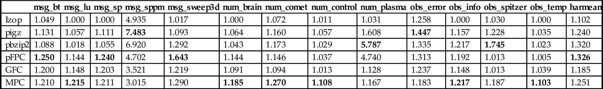
3.2 Compression Ratios
Tables 3 and 4 show the CRs on the double- and single-precision data sets, respectively, for the general-purpose compressors pbzip2 [17], pigz [18], and lzop [19], the special-purpose floating-point compressors pFPC [20] and GFC [21] (they only support double precision), and for MPC. The highest CR for each data set is highlighted in the tables. Because we wanted to maximize the CR, we selected the command-line flags that result in the highest CR where possible. For lzop we used –c6, as this is the highest compression level before the runtime becomes intractable. For pigz and pbzip2, we used –c9 –p20. For GFC and MPC, we specified the data-set dimensionality on the command line. GFC and MPC are parallel GPU implementations. pFPC, pbzip2, and pigz are parallel CPU implementations. The remaining compressor, lzop, is a serial CPU implementation.
All of the tested algorithms except lzop and GFC compressed at least one data set best. MPC delivered the highest CR on six double-precision and eight single-precision data sets. This was a rather surprising result given that MPC is “handicapped” by being constrained to only utilize GPU-friendly components that retain almost no internal state.
MPC proved to be superior to lzop and GFC, both of which it outperformed on most of the tested data sets in terms of CR. Moreover, GFC and pFPC did not support single-precision data. pFPC and pbzip2 outperformed MPC on average. However, this was the case only because of two data sets, msg_sppm and num_plasma, on which they yielded much higher CRs than MPC.
Most of the double-precision data sets were less compressible than the single-precision data sets. This was expected as the least significant mantissa bits tend to be the most random in floating-point values and many of those bits are dropped when converting from double to single precision.
3.3 Compression and Decompression Speed
Tables 5 and 7 list the double- and single-precision throughputs in gigabytes per second on the 13 data sets for all tested compressors. Tables 6 and 8 list the same information, but for decompression. As stated before, GFC and pFPC do not support single-precision data. For the GPU-based compressors, we show results for both the K40, which has a compute capability of 3.5, and the Titan X, which has a compute capability of 5.2.
Table 5
Double-Precision Compression Throughput in Gigabytes per Second
| msg_bt | msg_lu | msg_sp | msg_sppm | msg_sweep3d | num_brain | num_comet | num_ control | num_plasma | obs_error | obs_info | obs_spitzer | obs_temp | Average | |
| Izop | 0.573 | 0.629 | 0.624 | 0.391 | 0.623 | 0.626 | 0.561 | 0.624 | 0.435 | 0.200 | 0.576 | 0.215 | 0.595 | 0.513 |
| Pigz | 0.168 | 0.184 | 0.133 | 0.096 | 0.181 | 0.174 | 0.140 | 0.187 | 0.223 | 0.104 | 0.160 | 0.123 | 0.175 | 0.157 |
| pbzip2 | 0.040 | 0.047 | 0.038 | 0.028 | 0.038 | 0.043 | 0.046 | 0.035 | 0.009 | 0.041 | 0.029 | 0.052 | 0.031 | 0.037 |
| pFPC | 0.637 | 0.570 | 0.666 | 0.844 | 0.555 | 0.514 | 0.467 | 0.506 | 0.268 | 0.348 | 0.149 | 0.556 | 0.255 | 0.487 |
| GFC_35 | 42.20 | 30.75 | 45.96 | 44.20 | 19.92 | 22.47 | 17.01 | 25.27 | 5.559 | 9.848 | 2.999 | 31.39 | 6.327 | 23.38 |
| GFC_52 | 38.63 | 28.34 | 40.75 | 40.73 | 18.35 | 20.71 | 15.67 | 23.29 | 5.123 | 9.075 | 2.764 | 27.84 | 5.830 | 21.32 |
| MPC_35 | 13.46 | 13.70 | 13.63 | 13.54 | 13.39 | 13.40 | 13.43 | 13.60 | 13.23 | 13.40 | 12.79 | 13.59 | 13.12 | 13.40 |
| MPC_52 | 18.47 | 18.41 | 18.61 | 18.74 | 18.61 | 18.48 | 18.49 | 18.23 | 17.79 | 18.16 | 16.86 | 18.65 | 17.57 | 18.23 |

Bold values denote the best value in each column.
Table 6
Double-Precision Decompression Throughput in Gigabytes per Second
| msg_bt | msg_lu | msg_sp | msg_sppm | msg_sweep3d | num_brain | num_comet | num_ control | num_plasma | obs_error | obs_info | obs_spitzer | obs_temp | Average | |
| Izop | 0.674 | 0.810 | 0.811 | 0.523 | 0.771 | 0.805 | 0.687 | 0.804 | 0.580 | 0.435 | 0.689 | 0.442 | 0.759 | 0.676 |
| Pigz | 0.084 | 0.082 | 0.075 | 0.228 | 0.081 | 0.081 | 0.087 | 0.089 | 0.108 | 0.097 | 0.085 | 0.074 | 0.087 | 0.097 |
| pbzip2 | 0.145 | 0.125 | 0.138 | 0.383 | 0.121 | 0.116 | 0.125 | 0.122 | 0.152 | 0.110 | 0.063 | 0.148 | 0.089 | 0.141 |
| pFPC | 1.108 | 1.013 | 1.172 | 2.112 | 1.101 | 0.951 | 0.848 | 0.875 | 0.760 | 0.773 | 0.402 | 0.935 | 0.562 | 0.970 |
| GFC_35 | 53.67 | 39.11 | 58.45 | 56.21 | 25.33 | 28.58 | 21.63 | 32.14 | 7.070 | 12.52 | 3.814 | 39.93 | 8.046 | 29.73 |
| GFC_52 | 58.07 | 42.32 | 63.07 | 60.82 | 27.41 | 30.92 | 23.40 | 34.77 | 7.650 | 13.55 | 4.127 | 43.20 | 8.706 | 32.16 |
| MPC_35 | 19.25 | 19.06 | 19.31 | 19.09 | 18.87 | 18.87 | 18.94 | 18.73 | 18.10 | 18.85 | 17.40 | 18.76 | 18.21 | 18.72 |
| MPC_52 | 18.93 | 18.80 | 18.93 | 18.84 | 18.55 | 18.57 | 18.60 | 18.47 | 17.77 | 18.49 | 17.03 | 18.43 | 17.93 | 18.41 |

Bold values denote the best value in each column.
Table 7
Single-Precision Compression Throughput in Gigabytes per Second
| msg_bt | msg_lu | msg_sp | msg_sppm | msg_sweep3d | num_brain | num_comet | num_ control | num_plasma | obs_error | obs_info | obs_spitzer | obs_temp | Average | |
| Izop | 0.482 | 0.619 | 0.614 | 0.509 | 0.581 | 0.612 | 0.507 | 0.601 | 0.561 | 0.166 | 0.520 | 0.318 | 0.566 | 0.512 |
| Pigz | 0.160 | 0.171 | 0.142 | 0.477 | 0.161 | 0.152 | 0.134 | 0.176 | 0.168 | 0.053 | 0.130 | 0.087 | 0.146 | 0.166 |
| pbzip2 | 0.050 | 0.034 | 0.038 | 0.019 | 0.013 | 0.042 | 0.041 | 0.036 | 0.009 | 0.042 | 0.025 | 0.048 | 0.030 | 0.033 |
| MPC_35 | 13.25 | 13.20 | 13.17 | 13.22 | 13.17 | 13.17 | 12.93 | 13.05 | 12.43 | 12.71 | 11.83 | 13.17 | 12.67 | 12.92 |
| MPC_52 | 18.97 | 18.80 | 18.76 | 19.03 | 18.55 | 18.75 | 18.39 | 18.79 | 17.51 | 18.07 | 16.13 | 18.96 | 17.62 | 18.33 |

Bold values denote the best value in each column.
Table 8
Single-Precision Decompression Throughput in Gigabytes per Second
| msg_bt | msg_lu | msg_sp | msg_sppm | msg_sweep3d | num_brain | num_comet | num_ control | num_plasma | obs_error | obs_info | obs_spitzer | obs_temp | Average | |
| Izop | 0.653 | 0.812 | 0.801 | 0.503 | 0.768 | 0.787 | 0.656 | 0.794 | 0.701 | 0.333 | 0.597 | 0.555 | 0.705 | 0.667 |
| pigz | 0.082 | 0.082 | 0.073 | 0.240 | 0.079 | 0.079 | 0.088 | 0.085 | 0.085 | 0.089 | 0.081 | 0.070 | 0.081 | 0.093 |
| pbzi p2 | 0.128 | 0.112 | 0.131 | 0.408 | 0.137 | 0.109 | 0.110 | 0.108 | 0.097 | 0.089 | 0.047 | 0.117 | 0.060 | 0.127 |
| MPC_35 | 18.85 | 18.41 | 18.59 | 18.98 | 17.25 | 18.73 | 18.22 | 18.56 | 17.48 | 17.75 | 15.94 | 18.77 | 17.61 | 18.09 |
| MPC_52 | 18.57 | 18.17 | 18.36 | 18.72 | 17.13 | 18.45 | 17.87 | 18.35 | 17.34 | 17.68 | 15.83 | 18.55 | 17.44 | 17.88 |

Bold values denote the best value in each column.
lzop is the fastest CPU-based algorithm at compression and decompression, but it is still 28 times slower than MPC. Thus MPC not only compresses better than lzop but also greatly outperforms it in throughput.
pFPC, the overall best implementation in terms of CR (on the double-precision data), is roughly 18 times slower when running on 20 CPU cores than MPC. GFC is the fastest tested implementation (on the double-precision data sets). It is roughly 1.5–2 times faster than MPC, which is expected as GFC is essentially a two-component algorithm whereas MPC has four. However, GFC compresses relatively poorly. Importantly, the single- and double-precision compression and decompression throughput of MPC matches or exceeds that of the PCI-Express v3.0 bus linking the GPU to the CPU in our system, making real-time operation possible.
3.4 Compression and Decompression Energy
Tables 9 and 11 show the energy efficiency when compressing each of the 13 double- and single-precision inputs. Tables 10 and 12 show the same information, but for decompression. As stated before, pFPC does not support single-precision data. Also, the K20 Power Tool does not currently support measuring energy on the Titan X. Thus we provide energy measurements only for MPC_35.
Table 9
Double-Precision Energy Efficiency in Words Compressed per Micro-Joule
| msg_bt | msg_lu | msg_sp | msg_sppm | msg_sweep3d | num_brain | num_comet | num_ control | num_plasma | obs_error | obs_info | obs_spitzer | obs_temp | Average | |
| Izop | 0.755 | 0.827 | 0.820 | 0.516 | 0.817 | 0.822 | 0.737 | 0.820 | 0.569 | 0.266 | 0.748 | 0.285 | 0.777 | 0.674 |
| Pigz | 0.165 | 0.180 | 0.132 | 0.101 | 0.178 | 0.170 | 0.142 | 0.183 | 0.222 | 0.105 | 0.162 | 0.122 | 0.173 | 0.157 |
| pbzip2 | 0.040 | 0.045 | 0.039 | 0.026 | 0.038 | 0.042 | 0.046 | 0.036 | 0.008 | 0.042 | 0.030 | 0.051 | 0.032 | 0.037 |
| pFPC | 0.597 | 0.532 | 0.631 | 0.876 | 0.562 | 0.487 | 0.432 | 0.456 | 0.282 | 0.342 | 0.152 | 0.519 | 0.246 | 0.470 |
| MPC_35 | 44.53 | 30.37 | 46.54 | 56.14 | 53.56 | 52.80 | 117.67 | 52.10 | 4.134 | 3.942 | 6.379 | 43.46 | 4.840 | 39.73 |

Bold values denote the best value in each column.
Table 10
Double-Precision Energy Efficiency in Words Decompressed per Micro-Joule
| msg_bt | msg_lu | msg_sp | msg_sppm | msg_sweep3d | num_brain | num_comet | num_ control | num_plasma | obs_error | obs_info | obs_spitzer | obs_temp | Average | |
| Izop | 0.887 | 1.061 | 1.064 | 0.697 | 1.014 | 1.054 | 0.906 | 1.053 | 0.753 | 0.576 | 0.903 | 0.586 | 0.992 | 0.888 |
| pigz | 0.108 | 0.105 | 0.097 | 0.292 | 0.104 | 0.105 | 0.111 | 0.113 | 0.138 | 0.125 | 0.109 | 0.095 | 0.111 | 0.124 |
| pbzip2 | 0.134 | 0.116 | 0.128 | 0.348 | 0.114 | 0.109 | 0.119 | 0.114 | 0.146 | 0.106 | 0.067 | 0.136 | 0.088 | 0.133 |
| pFPC | 1.190 | 1.086 | 1.267 | 2.249 | 1.200 | 1.019 | 0.909 | 0.932 | 0.820 | 0.835 | 0.445 | 1.003 | 0.613 | 1.044 |
| MPC_35 | 43.64 | 31.80 | 47.52 | 45.70 | 20.60 | 23.23 | 17.58 | 26.13 | 5.748 | 10.18 | 3.101 | 32.46 | 6.541 | 24.17 |

Bold values denote the best value in each column.
Table 11
Single-Precision Energy Efficiency in Words Compressed per Micro-Joule
| msg_bt | msg_lu | msg_sp | msg_sppm | msg_sweep3d | num_brain | num_comet | num_control | num_plasma | obs_error | obs_info | obs_spitzer | obs_temp | Average | |
| Izop | 1.273 | 1.621 | 1.605 | 1.328 | 1.520 | 1.605 | 1.336 | 1.572 | 1.450 | 0.438 | 1.383 | 0.841 | 1.490 | 1.343 |
| Pigz | 0.317 | 0.339 | 0.282 | 0.973 | 0.319 | 0.300 | 0.289 | 0.346 | 0.341 | 0.112 | 0.270 | 0.175 | 0.294 | 0.335 |
| pbzip2 | 0.097 | 0.070 | 0.076 | 0.037 | 0.026 | 0.085 | 0.084 | 0.074 | 0.017 | 0.085 | 0.057 | 0.094 | 0.064 | 0.067 |
| MPC_35 | 50.94 | 165.1 | 51.53 | 84.31 | 119.36 | 90.32 | 107.7 | 93.18 | 6.239 | 7.929 | 3.620 | 79.42 | 3.206 | 66.37 |

Bold values denote the best value in each column.
Table 12
Single-Precision Energy Efficiency in Words Decompressed per Micro-Joule
| msg_bt | msg_lu | msg_sp | msg_sppm | msg_sweep3d | num_brain | num_comet | num_control | num_plasma | obs_error | obs_info | obs_spitzer | obs_temp | Average | |
| Izop | 1.708 | 1.621 | 1.605 | 1.328 | 1.520 | 1.605 | 1.336 | 1.572 | 1.450 | 0.438 | 1.383 | 0.841 | 1.490 | 1.377 |
| pigz | 0.210 | 0.339 | 0.282 | 0.973 | 0.319 | 0.300 | 0.289 | 0.346 | 0.341 | 0.112 | 0.270 | 0.175 | 0.294 | 0.327 |
| pbzi p2 | 0.242 | 0.070 | 0.076 | 0.037 | 0.026 | 0.085 | 0.084 | 0.074 | 0.017 | 0.085 | 0.057 | 0.094 | 0.064 | 0.078 |
| MPC_3S | 49.43 | 109.7 | 45.83 | 82.37 | 10.37 | 10.46 | 19.92 | 135.6 | 7.269 | 8.488 | 2.082 | 65.69 | 2.772 | 42.31 |

Bold values denote the best value in each column.
We can clearly see that MPC dominates the CPU compressors in terms of energy efficiency. For the CPU compressors, lzop is best for double- and single-precision compression as well as single-precision decompression, while pFPC is best for double-precision decompression.
Data compression on the GPU is between 1.8 to over 80 times more energy efficient than even the most energy efficient of the tested CPU compressors. Furthermore, it appears that decompression is more energy efficient on average than compression for lzop, pbzip2, and pFPC. For pigz and MPC, compression is more efficient than decompression, though on average, MPC decompression is still over 25 times more energy efficient than CPU decompression.
3.5 Component Count
Fig. 3 illustrates by how much the CR is affected when changing the number of chained components on the double-precision data sets. The bars marked “Best” refer to the single algorithm that yields the highest harmonic-mean CR over all 13 data sets. The other bars refer to the best algorithm found for each individual data set. We used exhaustive search for up to four-component algorithms. Because the runtime of exhaustive search is exponential in the number of components, we had to use a different approach for algorithms with more than four stages. In particular, we chose a genetic algorithm to find good (though not generally the best) algorithms in those vast search spaces. The single-precision results are not shown as they are qualitatively similar.
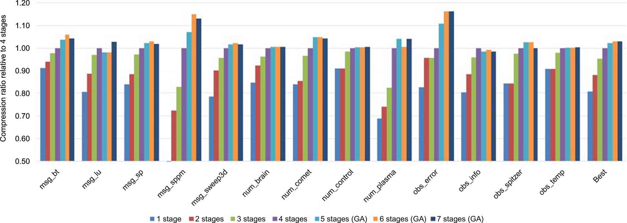
Except on two data sets, a single-component suffices to reach roughly 80–90% of the CR achieved with four components. Moreover, the increase in CR when going from one to two stages is generally larger than going from two to three stages, which in turn is larger than going from three to four stages, and so on. For example, looking at the harmonic mean, going from one to two stages, the CR improves by 8.9%; going from two to three stages, it improves by 8.4%, then by 4.8%, 2.3%, and 0.7%; and going from six to seven stages, the harmonic mean does not improve any more at all (which is in part because of the genetic algorithm not finding better solutions). In other words, the improvements start to flatten out, that is, algorithms with large numbers of stages do not yield much higher CRs and are slower than the chosen four-stage algorithms. Note that, due to the presence of the NUL component, the algorithms that can be created with a larger number of stages represent a strict superset of the algorithms that can be created with fewer stages. As a consequence, the exhaustive-search results in Fig. 3 monotonically increase with more stages. However, this is not the case for the genetic algorithm, which does not guarantee finding the best solution in the search space.
4 Summary and Conclusions
The goal of this work is to determine whether effective algorithms exist for floating-point data compression that are suitable for massively parallel architectures. To this end, we evaluated millions of possible combinations of 24 GPU-friendly algorithmic components to find the best algorithm for each tested data set as well as the best algorithm for all 13 data sets together, both for single- and double-precision representations. This study resulted in well-performing algorithms that have never before been described. A detailed analysis thereof yielded important insights that helped us understand why and how these automatically synthesized algorithms work. This, in turn, enabled us to make predictions as to which algorithms will likely work well on other data sets, which ultimately led to our MPC algorithm. It constitutes a generalization of the best algorithms we found using exhaustive search and requires only two generally known parameters about the input data: the word size (single- or double-precision) and the dimensionality.
It rivals the CRs of the best CPU-based algorithms, which is surprising because MPC is limited to using only algorithmic components that can be easily parallelized and that do not use much internal state. In contrast, some of the CPU compressors we tested utilize megabytes of internal state per thread. We believe the almost stateless operation of MPC make it a great algorithm for any highly parallel compute device as well as for FPGAs and hardware implementations, for instance in an NIC.
Our open-source implementation of MPC, which is available at http://cs.txstate.edu/~burtscher/research/MPC/, greatly outperforms all other tested algorithms that compress similarly well in compression and decompression throughput as well as in energy efficiency. Moreover, the throughput of MPC is sufficient for real-time compression/decompression of data transmitted over the PCIe bus or a LAN. Clearly, highly parallel, effective compression algorithms for floating-point data sets do exist.