
14 Planning Reliability of an Aging System
14.1 INTRODUCTION
An aging infrastructure will have a detrimental effect on a utility’s customer service reliability. Gradually, as equipment deteriorates and equipment failure rates increase, the rate of service interruptions will begin to increase. All measures of customer service reliability – SAIFI, SAIDI, MAIFI and others, will inevitably worsen. An old, partially worn-out power system is inherently less reliable, in terms of customer service quality, than a new one.
It is not possible to add enough Smart equipment and “self healing capability,” enough automated switching, and enough fault location and diagnostic equipment to guarantee this escalation in service interruptions and SAIDI and SAIFI problems can be completely controlled. A utility cannot “fix” the reliability problems created by aging by focusing only on technology alone.
Aging Actually Creates An Opportunity for More Reliability Improvement
As a system becomes inherently less reliable due to aging, the effectiveness of many reliability improvement methods increases. In a system where SAIFI is expected to be .66, certain automated switching and fault location programs may not provide a benefit/cost ratio of 1.00 or more. There is not enough opportunity, in such a reliable system, for them to justify their expense. But if the SAIFI is 1.33, they are about twice as cost effective. Therefore, as a system ages and failure rates increase, the cost effectiveness of various reliability improvement methods gradually rises. And as more is spent to renew equipment, the cost effectiveness of reliability improvement methods drops.
What a utility wants is the lowest cost way to deliver satisfactory service reliability to its customers. To the customer, it does not matter if that reliability comes from an a network composed of worn out equipment that is controlled smartly by an advanced monitoring and control system, or from a network that is inherently reliable because equipment condition is maintained at a high level. What is important is that: a) service is reliable, and b) cost is as low as possible. The industrial power owner seeks the same cost “sweet spot.”
Not surprisingly, in every case, the lowest cost, lowest risk plan is always a combination of both approaches, something that basically picks the low hanging fruit from each method in order to provide just enough reliability to satisfy needs. Thus, reliability engineering – planning, specification, and implementation of measures to improve and control customer reliability – is an important aspect of planning for aging infrastructures. The other part is the planning of the best inspection, tracking, condition improvement, life extension, proactive replacement plan. The two interact, creating synergy if used together well and problems if not, so they must be planned in conjunction with one another.
Reliability Engineering of Power Delivery
This chapter summarizes power delivery reliability concepts and methods.
The goal of reliability-based planning, engineering, and operations is to cost effectively maximize reliability of service as seen by the customer, not necessarily to improve reliability of equipment or service time on the system. Customer-level results are what count.
While equipment availability and similar measures are important, the planning and engineering process should focus on customer-level measures of service reliability.
Why is Reliability More Important Today Than It Was Traditionally?
Distribution system reliability is driven by several factors including:
(1) The increasing sensitivity of customer loads to poor reliability, driven both by the increasing use of digital equipment, and changing lifestyles.
(2) The importance of distribution systems to customer reliability as the final link to the customer. They, more than anything else, shape service quality.
(3) The large costs associated with distribution systems. Distribution is gradually becoming an increasing share of overall power system cost.
(4) Regulatory implementation of performance based rates, and large-customer contracts that specify rebates for poor reliability, all give the utility a financial interest in improving service quality.
In the past, distribution system reliability was a by-product of standard design practices and reactive solutions to historical problems. In the future, distribution system reliability will be a competitive advantage for a distribution utility, in its competition with other forms of power and energy (DG, alternate fuels, and conservation). Reliability must be planned for, designed for, optimized, and treated with analytical rigor.
Optimal Reliability isn’t Necessarily Maximum Reliability
Planners must keep in mind that while reliability is important to all customers, so is cost, and that only a portion of the customer base is willing to pay a premium price for premium levels of reliability. The real challenge for a distribution utility is, within tight cost constraints, to:
• Provide a good basic level of reliability.
• Provide roughly equal levels of reliability throughout its system, with no areas falling far below the norm.
• Provide the ability to implement means to improve reliability at designated localities or individual customer sites where greater service quality is needed and justified.
In Section 14.2, this chapter will introduce an important concept: the engineering of reliability in a distribution system in the same way that other performance aspects such as voltage profile, loading, and power factor is engineered. Section
14.3 will summarize the analytical methods that can be used as the basis for such engineering and discuss their application. Section 14.4 gives an example of reliability-based engineering as applied to a medium-sized power system, designed for overall and site-specific targeted reliability performance. Financial risk, due to performance-based contracts and rates, is a big concern to a 21st century utility. Section 14.5 looks at the analytical methods needed to assess and optimize this, and shows an example analysis. Section 14.6 concludes with a summary of key points.
14.2 RELIABILITY CAN BE ENGINEERED
Figure 14.1 shows a screen from a computer program that can simultaneously assess voltage behavior, reliability, or cost of an arbitrary distribution system design input by the user – what is sometimes called a “reliability load flow.” The program bases its computations on an arc-node structure model of the system, very similar in concept, construction, and data, to that used in a standard load flow program. By using failure rate data on system components, the program can compute the expected number of outages that occur, and the expected total minutes of outage, annually, at each and every point in the network. From these results, indices such as SAIDI, SAIFI, CAIDI and CAIFI, or other reliability indices, can be computed for the network. The particular program shown has several characteristics important to practical application:
• It represents the impact of equipment failures on the interconnected system around it.
• It can model the actions of dynamic changes associated with a contingency, such as a fuse blowing, a breaker tripping, a rollover switch operating, or a line crew repairing a damaged line section.
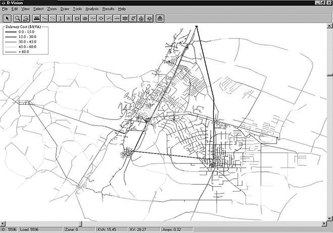
Figure 14.1 Screen display from a “reliability load flow” of the network in a small city. See text for details.
• It is self-calibrating. Given historical data on outage rates by portion of the system, it computes the failure rates for equipment in each area until its depiction of the base system’s reliability performance matches historical reality.
• It has a very large system capability, being able to analysis a distribution system composed of hundreds of thousands of nodes.
• Its model of the system itself (the circuit database) is in a standard load flow format compatible with most power system modeling.
• It is easy to use (graphic user interface).
Results are dependable
The results from this process as dependable from an engineering standpoint as those obtained from a well-applied load flow application. Generally, the reliability assessment has a better base of customer data than a load flow. It uses customer count data at the “load end” of the model (information that can be accurately determined) not kW load data (which are most typically estimates based on kWh sales).
Table 14.1 Reliability of Typical Types of Distribution System Components
Required component reliability data is not difficult to obtain
One of the primary concerns power system planners have with the use of a reliability-based engineering method is the data requirement. Such methods need data on the failure rates of various types of equipment, and repair and switching times for various situations. Generally, this data is available by culling through utility operating records. However, several sources of generic reliability data are available. These include default data obtained from industry standards (for example, Institute of Electrical and Electronics Engineers, International Conference on Large High Voltage Electric Systems), publications (such as books, journals, conference papers), and tests or surveys conducted by manufacturers. This information provides a good first guess and prepares the model to be calibrated against historical data. Table 14.1 lists typical values of failure rates for most common types of power system equipment.
As mentioned above, the best reliability-assessment programs have a self-calibrating feature: they “fit” their reliability analysis results to actual historical outage rates. These methods start with “generic” failure rate data in internal tables and make various adjustments and re-computations of what failure rates in an area must be, based on the historical data. Self-calibration is the best way to assure that a reliability-assessment model is accurate.
Results are useful even with only generic data
It is important to realize that a reliability-assessment method can help utility planning engineers improve the reliability performance of their system even if it is using approximate failure rate data. Most of the important decisions that are made with respect to reliability have to do with configuration, installation and location of protective and sectionalizing equipment, and switching. Even approximate data, used in accurate analysis of these issues, provides guidance on the wisdom of various decisions. Improvement can be made using only approximate (generic) failure rate and repair-time data.
Using a Reliability Load Flow
Planning engineers use a reliability-assessment program in much the same manner that they use a load flow to design the feeder system. They begin with performance targets - voltages and loadings with certain limits- for load flow planning, reliability within a certain range for reliability engineering. They then enter into the program a candidate system model, a data representation of the system as it is, or as they propose to build it.
The computer analysis then determines the expected performance of the system as represented to it. In a load flow, computing the expected voltages, flows, and power delivery at every point in the system does this. In a reliability assessment, computing the expected frequency and duration of outages at every point in the system does this.
The results are displayed for the user, usually graphically in a way that quickly communicates problems (results that are unacceptably out-of-range).
The planning engineers review the results. If they are less than desirable, they make changes to the system model, using the results as a guide to where improvements or changes should be made. The model is re-run in this manner until a satisfactory result is obtained.
Root Cause and Sensitivity Analysis
Root-cause analysis determines the contribution of each component to poor reliability. For example, if reliability is measured using SAIDI, a root-cause analysis will identify if pole failures, breaker failures, and so forth contribute what impact to the original cause of the SAIDI.
The analysis is considerably more important when part of an aging infrastructure program as well as a reliability augmentation plan. In a way it unites the two endeavors and it definitely provides a starting point to coordinate them well. Both the root-cause analysis, and the analysis of equipment failure trends (whether and how much they are increasing, etc.) are dealing with much the same data. An important point is whether aging of various types of equipment is a root cause. When it is, trends found that show a gradually increasing failure rates should be applied predictively based on the root case analysis: their contribution to reliability issues will worsen in company with those trends, etc.
In addition to knowing the contribution each component makes to the overall poor reliability of the system, it is desirable to know the impact that improving component reliability or design would have on the system’s reliability: again, this links reliability engineering and aging equipment analysis. Will a change make a difference?
For example, what would be the impact of reducing overhead line failures, reducing transformer failures, or reducing cable repair-time? A sensitivity analysis can be used to answer such questions: this simple approach adjusts a component parameter (such as its failure rate) by a small amount and records the corresponding change in system reliability.
Engineering the Design Improvements
In determining how to improve system performance, planning engineers focus on equipment or areas of the system that score high in terms of both root cause (they create a lot of the problems) and sensitivity (changes will make a difference on reliability). After a system has been modeled, calibrated, and examined with root cause and sensitivity analyses, potential design improvements can be identified and modeled. The focus should be on critical components – those with both high root-cause scores and high sensitivity scores.
14.3 Methods for Distribution System Reliability Assessment
Power distribution reliability can be designed just like any other aspect of performance – voltage profile, loading. Doing so in a dependable and efficient manner requires an engineering planning method that can simulate how any particular distribution design will perform in terms of reliability of service. The system reliability will be as targeted by the planners and the effort exerted does not require special skills or undue levels of effort.
Several suitable analytical methods for this type of engineering exist. In the same manner that a power flow model can predict the electrical behavior of a distribution system (such as currents and voltages), a computer program called a reliability assessment model, based on one of these methods, can predict the expected reliability performance of any particular distribution system. As reliability becomes more important to electric utilities and electricity consumers, these reliability assessment models will equal or surpass power flow models in importance and usage. Reliability models allow distribution engineers to
• Design new systems to meet explicit reliability targets,
• Identify reliability problems on existing systems,
• Test the effectiveness of reliability improvement projects,
• Determine the reliability impact of system expansion,
• Design systems that can offer different levels of reliability, and
• Design systems that are best suited for performance based rates.
Distribution system reliability assessment is a rapidly developing field. Some of the first work on computer programs for this was done at Westinghouse Advanced Systems Technology, Pittsburgh, in the late 1970s. One of the first commercial distribution system reliability analysis programs, PREL, came from that group in 1981. This software was mainframe based and not widely adopted, largely because utilities in the 1980s did not put the heavy emphasis on reliability as they do 20 years later.
Increasing sensitivity of customer loads and impending deregulation led several utilities to develop their own distribution reliability assessment capabilities in the early and mid-1990s. Demand for distribution reliability assessment software is continuing to grow and commercial packages are now available from several major vendors. Electric utilities that desire to apply such methods have no problem finding several suitable packages from which to choose.
Methodologies for Distribution System Reliability Analysis
Reliability assessment models work from an arc-node type database, very similar to that used in a distribution load flow program. Unlike a load flow, which uses data on each element to compute the interconnected flow of power through the system to the customer locations, the reliability assessment program uses data on each element to compute the interconnected reliability of service to the customer locations.
There are four common methodologies used for distribution reliability assessment: network modeling, Markov modeling, analytical simulation, and Monte Carlo simulation. These differ in their bases – in what they use as the foundation for their analysis of reliability. Each uses a different approach to determining the reliability of the system. A brief description of each is provided below.
Network modeling
Network modeling is based on the topology of the system, which it translates from a physical network into a reliability network based on serial and parallel component connections. Serial components have additive failure rates and each one can disable the entire chain. Parallel components have redundancy (up to a point corresponding to capacity) and can cover outages of other parallel pathways.
Network modeling basically takes the system topology and translates it into a “formula” of serial and parallel reliability characteristics, which it then uses to compute the reliability of the system performance. In computer models this formula is a table-driven set of equation coefficients that implements a reliability computation. This computation computes the likelihood that a continuous interconnection between a source, and the demand point, remains in operation.
Network modeling is simple and straightforward to implement, and produces good results at a basic evaluation of reliability. A major disadvantage for distribution system analysis is that dynamic functions, such as switching, or sequential system responses to contingencies, are outside of its context. Its formula applies to a basic topology, anything such as a switch operation that changes the topology, cannot be modeled. As such, it is not as widely used as other methods.
Markov modeling
Markov modeling is a powerful method for assessment of reliability, as well as for simulation of many other apparently random multi-state processes (such as wind and solar availability for renewable energy systems). Markov modeling is based on analyzing the states that a system could be in: states can be such things as “everything operating normally,” or “component one has failed,” or “component two has failed,” etc. It focuses, though, on analyzing the transitions between these states: it analyzes the likelihood that the system can move from the condition “everything is operating normally” to “component one has failed,” as well as under what conditions, and how long, it takes to transition back.
Every condition, or state, that the system could be in is identified and enumerated. The analytical method focuses on computing the back and forth transitions between one state and another. It models the conditions and likelihood of these transitions, thereby mapping the amount of time that the system spends in each state. If one state is “everything operating normally” and others represent one failure model or another, then the model can be used to analyze reliability-of-service and its causes.
Markov modeling is excellent for representing systems where details of the transition between states are known or are important. For example, planners may want to study how different repair and replacement part policies would impact the availability of a DG unit. Having a repairman at the DG site, or the parts already there so they do not have to be spent for, would clearly reduce the time to transition from “broken” to “working.” Markov models make it possible to focus in great detail on studying questions about how much such actions would impact reliability, because they focus on the mechanism of moving between states, not on the states themselves.
However, Markov models have some disadvantages for power distribution system applications. The first is that the states modeled are memory less (transition out of a state cannot depend on how the state was reached). This characteristic requires a type of duplication of states when system responses are a function of past events. Thus, if the system is in the state “working” because during the “broken” state a spare part was used (and as a result there no longer is another spare part at the site), the system cannot model this unless a new state is introduced: “working but no spare parts available.” Then, transitions between this state and “working” need to be established in the model (to represent delivery of the new part to the site). In practice, this complicates the application of a Markov model when used to analyze a distributed system such as a power distribution system.
The second limitation is computational. The matrix inversion required by Markov modeling requires that limits to the size of systems that can be represented and/or the complexity that can be represented to systems such as a few DG units. It also limits very simple distribution systems such as only the substation serving a small industrial site and its equipment.
Analytical simulation
Analytical simulation models each system contingency, computes the impact of each contingency, and weights this impact based on the expected frequency of the contingency. At first glance it appears to be very close to a form of contingency analysis, as was described in the Chapter 8 discussion on N-1 contingency analysis, except that likelihoods are assigned or computed for each contingency case. This is a big difference and not an easy one to add to N-1 analysis. Analytical simulation algorithms are built around the mechanism that computes the probability of each contingency case, rather than an explicit enumeration of contingency states, as in N-1 analysis.
Accurate reliability analysis using analytical simulation means computing the likelihood of each contingency based on failure rates and interconnection of equipment. Generally, dynamic functions of equipment such as fuses, breakers, rollover switches, etc., has to be modeled, too, hence the term “simulation.” A great advantage of this method is that such types of dynamic activity can be modeled.
If the likelihood of each contingency is computed based on a good representation of the failure rates and modes that would lead to it, this type of method can accurately model complex system behavior and dynamically enumerate each possible system state. Aggregation of system states and their probabilities then permits detailed assessment of reliability (all states that lead to success vs. failure).
Monte Carlo Simulation
Monte Carlo Simulation is similar to analytical simulation, but models random contingencies are based on probabilities of occurrence, rather than expected contingencies. This allows component parameters to be modeled with probability distribution functions rather than expected values.
Monte Carlo Simulation can model complex system behavior, non-exclusive events and produces a distribution of possible results rather than expected values (Brown et al., 1997). Disadvantages include computational intensity and imprecision (multiple analyses of the same system will produce slightly different answers). Additionally, Monte Carlo Simulation is not enumerative and may overlook rare but important system states.
Table 14.2 Results Computed By an Analytical Simulation
|
• Expected number of momentary interruptions (per year) • Expected number of sustained interruptions (per year) • Expected number of interrupted hours (per year) • Expected number of protection device operations (per year) • Expected number of switching operations (per year) |
For applications requiring determination of expected values of reliability, analytical simulation is the best method for distribution system assessment. It allows distribution engineers to quantify system reliability (SAIDI, SAIFI) over an entire system, and for individual customer locations, to calibrate models to historical data, to compare design alternatives, perform sensitivity analyses and to run optimization algorithms to maximize the expected results [See Brown, et al., 1998 - 2000]. Monte Carlo Simulation becomes necessary if statistical results other than expected values are required – analysis of such things as the distribution of expected SAIDI from year to year.
14.4 APPLICATION OF ANALYTICAL SIMULATION FOR DETAILED RELIABILITY ASSESSMENT
An analytical simulation method simulates a contingency, determines the impact of this contingency on system reliability, and weights the impact of the contingency by its probability of occurrence. This process is repeated for all possible contingencies, and results in the following information for each component, providing the results shown in Table 14.2.
Simultaneously with the analysis of each contingency and the results it produces, the analytical simulation method evaluates the probability of occurrence of this contingency – how likely is it to occur? Once all contingencies have been analyzed, their results are combined appropriately on a probability-weighted basis to produce aggregate results. In distribution system analysis this aggregation of results is based on system topology, keyed to adjacent equipment, branches, circuits, etc., as well as the entire system.
Modeling Each Contingency
A contingency occurring on a distribution system is followed by a complicated sequence of events. Each contingency may impact many different customers in many different ways. In general, the same fault will result in momentary interruptions for some customers and varying lengths of sustained interruptions for other customers, depending on how the system is switched and how long the fault takes to repair. The key to an analytical simulation is to accurately model the sequence of events after a contingency to capture the different consequences for different customers. A generalized sequence of events as modeled by analytical simulation is:
1. Contingency: A fault occurs on the system.
2. Reclosing: A reclosing device opens in an attempt to allow the fault to clear. If the fault clears, the reclosing device closes and the system is restored to normal.
3. Automatic Sectionalizing: Automatic sectionalizers that see fault current attempt to isolate the fault by opening when the system is de-energized by a reclosing device.
4. Lockout: If the fault persists, time over current protection clears the fault. Lockout could be the same device that performed the reclosing function, or could be a different device that is closer to the fault.
5. Automated Switching: Automated switches are used to quickly isolate the fault and restore power to as many customers as possible. This includes both upstream restoration and downstream restoration. In upstream restoration, a sectionalizing point upstream from the fault is opened. This allows the protection device to reset and for restoration of all customers upstream of the sectionalizing point. In downstream restoration, other sections that remain de-energized are isolated from the fault by opening switches. Customers downstream from these points are restored through alternate paths by closing normally-open tie switches.
6. Manual Switching: Manual switching restores power to customers that could not be restored by automated switching (certain customers will not be able to be restored by either automated or manual switching). As in automated switching, manual switching has both an upstream restoration component and a downstream restoration component.
7. Repair: The fault is repaired and the system is returned to its pre-fault state.
The seven steps outlined above generate a set of system states for each contingency. Switches and protection devices being open or closed characterize these states. For each state occurring with frequency l and duration q, the accrued outage frequency of all de-energized components are incremented by l (if the component was energized in the preceding state) and the accrued outage duration of all de-energized components are incremented by l x q.
The simulation becomes more complicated if operational failures are considered. Operational failures occur when a device is supposed to operate, but fails to do so. The probability of such an event is termed probability of operational failure, POF. Operational failures cause the simulation sequence to split. One path assumes that the device fails to operate and has a weight of POF, the other path assumes that the device operates and has a weight of 1 – POF. This path splitting is illustrated in Figure 14.2, which shows the steps required when considering a fuse that is supposed to clear a fault.
The result of simulation path splitting is an enumerative consideration of all possible system responses to each contingency (in the context of operational failures). Enumerative consideration is important since some states may be rare, but have a major impact on the system when they do occur. During restoration, path splitting associated with the enumerative consideration of possible outcomes is important when intended switching fails and customers that would otherwise have been restored are not.

Figure 14.2 Simulation path splitting due to operational failures.
Incremental Studies of Improvement
An analytical simulation will produce identical results if an analysis is performed multiple times. In addition, small changes in input data will cause small changes in results (as opposed to some other methods). This allows the impact of small reliability improvements to be quantified for individual customers and reliability indices by running a series of studies of incremental changes in the system design. For example, the planning engineer can move the location of a sectionalizer or recloser up and down a feeder an eighth of a mile at a time, seeing the results in total reliability, and the distribution of reliability results up and down the feeder, with each change. This capability also allows input parameters to be perturbed and result sensitivities to be computed. However, analytical simulation does not allow the uncertainty of reliability to be quantified. For example, while expected that SAIDI might be 2.0 hours per year, there is some probability that next year will just be an “unlucky year.” To compute how often such unlucky years could occur, and how extreme SAIDI or other factors would be in those years, requires application of Monte Carlo techniques.
Example Application
An analytical simulation method was applied to the test system shown in Figure 14.1, which is based on an actual U.S. utility distribution system. The system model contains 3 voltage levels, 9 substations, more than 480 miles of feeder, and approximately 8,000 system components. The model was first calibrated to historical outage data, then used to analyze candidate designs as described above. In addition the authors used an optimization module that maximized reliability results versus cost. The diagram shown in Figure 14.1 was originally color coded (not shown here) based on computed outage hours, and shows the system plan that resulted from a combination of engineering study and use of optimization. Individual component reliability results can be easily used to generate a host of reliability indices. For this system, common indices include:
MAIFI (Momentary Average Interruption Frequency Index) = 2.03 /yr
SAIFI (System Average Interruption Frequency Index) = 1.66 /yr
SAIDI (System Average Interruption Duration Index) = 2.81 hr/yr
Targets for the area were 2.00, 1.75, and 2.9 hours (175 minutes) respectively, thus this system essentially meets its target reliability criteria.
Differentiated Reliability Design
Realistically, the expected reliability of service over an entire distribution system cannot be the same at all points. Distribution systems use transshipment of power through serial sets of equipment. Thus there are areas of the system that are more “downstream,” and being downstream of more devices and miles of line, have somewhat higher exposure to outage. Figure 14.1’s example demonstrates this. Although SAIDI is 2.81, expected performance for the best 5% of customers is
1.0 hours and 4.02 for the worst 5%.
However, planning engineers can engineer a system to keep the range of variation in what customers in one area receive versus customers in another, with within a reasonable range. This involves the selected use of protective equipment such as fuses and breakers, sectionalizers, reclosers, and contingency switching plans, and in some cases, distribution resources such as on-site generation and energy storage, and demand-side management. Artful use of these measures, combined with application of sound distribution layout and design principles, should result in a system that provides roughly equitable service quality to all customers.
However, there are situations where a utility may wish to promise higher than standard reliability to a specific customer, or to all customers in an area such as a special industrial park. These situations, too, can be engineered. In fact, generally it is far easier to engineer the reliability of service to a specific location than it is to engineer an entire system to a specific target.
Performance-Based Industrial Contracts
Generally, such situations arise in the negotiation for service to medium and large industrial customers. Many of these customers have special requirements that make continuity of service a special consideration. All of them pay enough to the utility to demand special attention – at least to the point of having the utility sit down with them to discuss what it can do in terms of performance and price.
Figure 14.3 Service to three industrial customers in the example system were designed to higher-than-normal reliability performance targets.
The actual engineering of the “solution” to an industrial customer’s needs is similar to that discussed above for systems as a whole. Planning engineers evaluate the expected reliability performance of the existing service to the customer, and to identify weaknesses in that system. Candidate improvement plans are tried in the model, and a plan evolves through this process until a satisfactory solution is obtained. The system design in Figure 14.1 includes three such customer locations, as shown in Figure 14.3. Special attention to configuration, fusing and protection coordination on other parts of the circuit, contingency (backup) paths and quick rollover switching, provided about 80% of the improvement in each case.
The other 20% came from extending the reliability assessment analysis to the customer’s site. In each case, the customer’s substation, all privately owned, was analyzed and suggested improvements in equipment or configuration were recommended to his plant engineer. In one case the analysis extended to primary (4 kV) circuits inside the plant. Table 14.3 gives the results for each. For site A, the target has been exceeded in practice to date because there have been no outages in three years of operation. However eventually performance will probably average slightly better than the target, no more.
In the case of site B, the customer’s main concern was that the length of any interruption be less than a quarter hour. Thus, the target is not aimed at total duration time, but on each event, something quite easy to engineer. Performance has greatly beaten this target – means to assure short outages such as automatic rollover and remote control restore power in much less time than required.
For customer C, any interruption of power resulted in loss of an entire shift’s (eight hours’) production. Thus, the major item of interest there was total count of events. Initial evaluation showed little likelihood of any interruption lasting that long. Reliability engineering focused on frequency only.
Table 14.3 Reliability Targets for Three Special Customers
In all three cases, the performance-based contracts call for a price to be paid that can be considered a premium service price. It is typical for industrial customers in this class to negotiate price and conditions with the utility, but in all three cases the price included an identified increment for the improvement in service. Unlike some performance-based rate schedules, there is no “reward” or extra payment for good service – the premium payment is payment for the good service.
But performance penalties are assessed, not on an annual basis depending on annual performance, but on an event basis. If reliability of service is perfect, the utility has earned all the premium monies paid. Any event (any, not just those exceeding the limits) garners a rebate according to a certain formula. For example, customer B receives a $30,000 rebate for any interruption of power, but the rebate rises to $300,000 if the interruption lasts more than 30 minutes. (Customer B’s average monthly bill is about $175,000.)
14.5 USE OF A HYBRID ANALYTICAL SOLUTION
If one hundred identical distribution systems are built, the expected reliability of each will be identical. In a given year, some of these systems might be lucky and experience nearly perfect reliability. Others may experience near expected reliability, and others may be unlucky and experience far worse than expected reliability. This variation is natural and is vital to understand when negotiating reliability-based contracts.
Variations in reliability can be examined using techniques referred to as risk assessment methods. A risk assessment model identifies all possible outcomes. and the
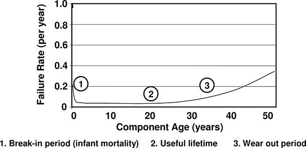
Figure 14.4 The traditional “bathtub” failure rate curve, as discussed in the text. Here, the device has a useful lifetime of about 30 – 35 years.
This commonly takes the form of a probability of each outcome occurring. When possible, this is done through analytical methods such as function convolution. However, often this is not feasible and “Sequential Monte Carlo Simulation” is used where time slices are modeled in succession and each component is tested for random failures during each time slice. This type of simulation is very flexible and can handle complex models, but is computationally slow and data intensive.
Many of the problems associated with a sequential Monte Carlo Simulation can be overcome if components are assumed to have a constant failure rate over the course of one year. This is a reasonable assumption and can be visualized by “bathtub failure rate functions.” These functions show that typical electrical components will have a high failure rate when they are first installed (due to manufacturing defects, damage during shipping, and improper installation). The failure rate will reduce after this “infant mortality” period and remain at a fairly constant level over the useful life of the component. The failure rate will gradually rise as the equipment wears out at the end of its useful life. A bathtub failure rate function is shown in Figure 14.4.
Components with constant failure rates follow a Poisson process. This allows the probability of the component failing a specific number of times in a year to be easily computed. If a component has a constant failure rate of l times per year, the probability of it failing x times in a year is:
![]()
If constant failure rates are assumed, the analytical simulation described in the previous section can be modified to simulate a random year rather than an expected year. This is done by determining the number of times each component will fail a priori. For each component, a random number between zero and one is generated. If this number is less that e-l, no failure will occur in the year being simulated. If the random number is greater, the number of times that the component will fail is determined by Equation 1.
Once the number of times each component will fail is determined, an analytical simulation is performed that substitutes component failure rates with the number of times that they will fail in the random year being simulated. Using this process, many years can be simulated, a list of outcomes can be recorded, and distribution statistics can be computed. This methodology is referred to as an Analytical/Monte Carlo Hybrid Simulation. This particular hybrid simulation has two desirable features:
1. It requires no additional data beyond the requirements of an analytical model. !
2. If there is confidence in the expected values generated by the analytical simulation, and there is confidence that component failure rates are constant over a single year; there is equal confidence in the results of the analytical/Monte Carlo hybrid simulation.
Analytical/Monte Carlo Hybrid Simulation is applied to the system being analyzed (i.e., the system in Figures 14.1 and 14.3) by performing 1,000 random simulations on the same system that was used to demonstrate the analytical simulation. The results are shown in Figure 14.5 as both a histogram (the bar chart) and an integral of the histogram (the continuous line). The statistical results of the simulation are (in hours per year): mean value = 2.81, standard deviation =.79, minimum value = .95, maximum value = 6.37.
The Analytical/Monte Carlo Hybrid Simulation is computationally intensive, but provides statistical results not obtainable by using purely analytical methods. This statistical information is vital when assessing technical and financial risk associated with reliability based contracts. The remainder of this chapter demonstrates this by applying Analytical/Monte Carlo Hybrid Simulations to distribution systems subject to performance based rates.
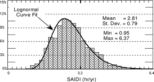
Figure 14.5 SAIDI Results for 1,000 random years (hr/yr). Bars show a histogram of the expected annual results, which, while having a mean of less than 3 hours, have a good probability of being over 5 hours. Solid fits a log-normal curve to the data.
Analyzing the Risk from Performance-Based Rates
Deregulated utilities are reducing costs by deferring capital projects, reducing in-house expertise, and increasing maintenance intervals. As a direct consequence, the reliability on these systems is starting to deteriorate. Since these systems have been designed and maintained to high standards, this deterioration does not manifest itself immediately. System reliability will seem fine for several years, but will then begin to deteriorate rapidly. When reliability problems become evident, utilities often lack the necessary resources to address the problem.
Regulatory agencies are well aware that deregulation might have a negative impact on system reliability. In a perfect free market, this would not be a concern. Customers would simply select an electricity provider based on a balance between price and reliability. In reality, customers are connected to a unique distribution system that largely determines system reliability. These customers are captive, and cannot switch distribution systems if reliability becomes unacceptable. For this reason, more and more utilities are finding themselves subject to performance-based rates (PBRs).
A PBR is a contract that rewards a utility for providing good reliability and/or penalizes a utility for providing poor reliability. This can either be at a system level based on reliability indices, or can be with individual customers. Performance is usually based on average customer interruption information. This typically takes the form of the reliability indices SAIFI and SAIDI.
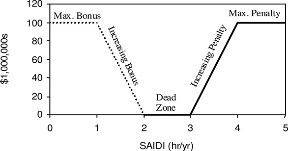
Figure 14.6 Performance based rate structure for the example in this section. There is no penalty or incentive payment for annual SAIDI performance that lies between 2 and 3 hours. Above that the utility pays a penalty of $1,666,666 per minute, up to 60 minutes. Similarly, it receives a reward of the same magnitude for each minute below the dead zone.
A common method of implementing a PBR is to have a “dead zone” where neither a penalty nor a bonus will be assessed. If reliability is worse than the dead zone boundary, a penalty is assessed. Penalties increase as performance worsens and are capped when a maximum penalty is reached. Rewards for good reliability can be implemented in a similar manner. If reliability is better than the dead zone boundary, a bonus is given. The bonus grows as reliability improves and is capped at a maximum value. All PBRs will have a penalty structure, and some will have both a penalty structure and a bonus structure. A graph of a PBR based on SAIDI is shown in Figure 14.6.
Most initial PBRs will be negotiated by the utility to be “easy to meet.” This means that business as usual will put the utility in the dead zone. This does not mean that a utility should do business as usual. It may want to spend less on reliability until marginal savings are equal to marginal penalties. Similarly, it may want to spend more money on reliability until marginal costs are equal to the marginal rewards. In either case, a utility needs a representative reliability assessment and risk model to determine the impact of reliability improvement and cost reduction strategies.
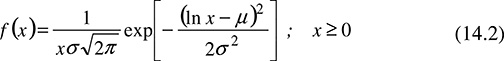
In order to make intelligent decisions about PBRs based on average system reliability, a probability distribution of financial outcomes is needed. This requires a PBR structure (such as the one shown in Figure 14.6) and a distribution of relevant reliability outcomes (like the histogram shown in Figure 14.5). It is also desirable to describe the reliability histogram with a continuous mathematical function. A good function to use for reliability index histograms is the log-normal distribution, represented by f(x):
The parameters in this equation can be determined by a host of curve-fitting methods, but a reasonably good fit can be derived directly from the mean and variance. If a mean value, x, and a variance are computed, log-normal parameters are:
![]()
![]()
The log-normal curve corresponding to the test system is shown along with the histogram in Figure 14.5. The curve accurately captures the features of the histogram including the mean, median, mode, standard deviation, and shape.
Assume that a system analyzed earlier, characterized by the reliability shown in Figure 14.5, is subject to the PBR formula shown in Figure 14.6. Using these two functions, a financial risk analysis can be easily determined. For example, the expected penalty will be equal to:
The probability of certain financial outcomes can also be computed. For example, the probability of landing in the dead zone will be equal to the probability of have a SAIDI between 2 hours and 3 hours. This is mathematically represented by:
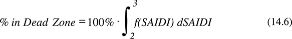
The expected outcome of the test system is $14 million in penalties per year. Thus, despite the fact that the expected annual SAIDI (2.81 hours) lies in the dead zone (no penalty – no reward) the utility will on average have to pay a fine amounting to about 8.4 minutes per year. Penalties will occur 32% of the time, bonuses will occur 12% of the time, and the utility will be in the Dead Zone 57% of the time. The distribution of all possible outcomes and their associated probabilities is shown in Figure 14.7.
For a cash-strapped utility, Figure 14.7 represents an unwelcome situation. And it is risky, because even though the average penalty of $14 million may be acceptable, that outcome will rarely happen. The $14 million average occurs because a penalty of $50 million or more will occur once every 7 years and the maximum penalty of $100 million will occur once every 12 years. Faced with this situation, a utility would be wise to negotiate a less risky PBR. Possibilities for adjusting the PBR to mitigate risk include:
1. Make the reward and penalty slopes less steep,
2. Widen the dead zone boundaries,
3. Move the dead zone to the right, and
4. Reduce bonus and penalty caps. Each of these options can be used alone, or a combination can be negotiated.
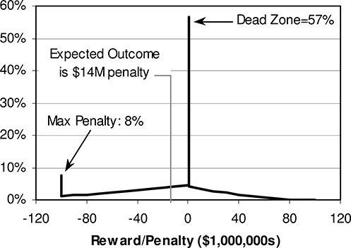
Figure 14.7 Distribution of financial outcomes for the example PBR problem. Although it is most likely the penalty/reward is zero (performance lies in the dead zone) the utility has a significant probability of getting hit with the maximum penalty (about once in every 12 years), while no chance of getting the maximum reward.
A suggested change to the PBR rules to mitigate the risk for this utility system is shown in Figure 14.8. This change stretches out the bonus and penalty transition zones from one hour to two hours. The impact of this changed PBR on the utility’s expected financial exposure is shown in Figure 14.9. On the surface, it may seem like not much has changed. Penalties will still occur 32% of the time, bonuses will still occur 12%, but total risk is reduced greatly, by $5 million. Utility companies can use predictive reliability assessment tools when planning and designing their systems and their responses to regulatory rules. This will allow the reliability of existing systems to be assessed, the reliability impact of projects to be quantified, and the most cost-effective strategies to be implemented. In most cases, an analytical model (Chapter 14) will be sufficient. This will allow utilities to compare the expected performance of various systems and various design options. Analytical/Monte Carlo hybrid techniques become necessary when technical and financial risk needs to be examined. This chapter has shown methodologies to serve both of these need categories.
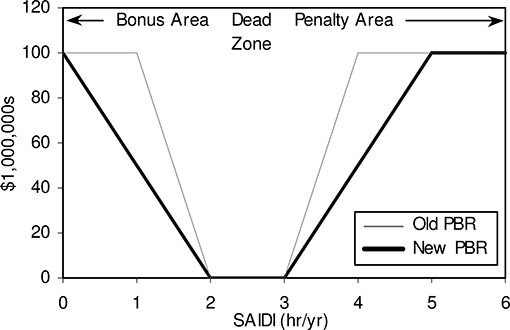
Figure 14.8 Changed PBR schedule that reduces risk. The schedule has a milder rise in both penalty and reward sides and is a “fair” proposal for the utility to make to regulators because it treats both penalty and reward sides equally.
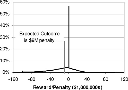
Figure 14.9 Financial outcome with the revised PBR formula. The utility’s expected average is still a penalty, but only $9 million, an improvement of $5 million. More important, the possibility of it being hit with a large (over $50 million) penalty has decreased greatly.
14.6 CONCLUSION AND KEY POINTS
The reliability of service of a power distribution system can be designed to meet specific goals with respect to reliability criteria such as SAIDI and SAIFI. It can also be designed to minimize financial risk whether that is measured in terms of utility and/or customer costs, or includes performance-based rates and contracts as well. Of four possible methods, all capable of computing distribution reliability, the authors believe the analytical simulation method is most applicable to reliability-based planning.
Analytical simulation computes the expected reliability of each component based on system topology and component reliability data. It does so by simulating the system’s response to each contingency, determining the impact of this contingency to each component, and weighting the impact of each contingency by its probability of occurrence. The result for each component is the expected number of momentary interruptions per year, the expected number of sustained interruptions per year, and the expected number of outage hours per year. Results can be displayed in tables, visualized spatially, or aggregated into reliability indices.
To assess technical and financial risk, the analytical simulation method is expanded to an Analytical/Monte Carlo Hybrid Simulation. Such a method assumes that component failure rates are constant over a specific year and models many random years rather than a single expected year. The result is a probability distribution of possible results that can be used to obtain information such as variance, median, modality, shape, and extremes. It also allows rigorous risk analyses to be performed on various types of performance-based rates and customer contracts.
After negotiating a performance-based rate, a distribution utility will find itself in a radically new paradigm. An explicit dollar value has been placed on reliability, and systems can be designed to balance the cost of reliability with the cost of infrastructure. If reliability measures are based on indices such as SAIFI and SAIDI, it may be beneficial to the utility to allow the reliability of a few customers in areas where it would be expensive to “fix” problems to decline to levels far below average.
Every power system will have areas where reliability can be improved relatively inexpensively, where for whatever reason the marginal cost of SAIDI and SAIFI improvement is low. Focusing on these areas alone improves overall utility-wide statistics, but increases the variance of customer experience. Eventually, this global “gaming” of the performance criteria will be viewed as unacceptable by customers and regulators alike, sparking more complicated PBR formulas and regulations designed to prevent such situations. Ironically, “deregulation” may therefore result in regulation of a previously unregulated area. It is best to focus on comprehensive programs that keep customer service everywhere within rather tight bounds. Regardless, reliability can be engineered. Key aspects of reliability-based engineering for distribution systems are:
• Focus on a customer-oriented metric. What really counts is the reliability of service the customer sees not reliability as measured on the power system itself. Reliability-based engineering should target customer-level reliability performance.
• Use a good reliability-assessment method. Such methods apply a rigorous analytical method, compute expected reliability on a detailed (nodal) basis, and use a method that provides consistent evaluation of results so that the effect of incremental design changes can be seen.
• Use differentiated reliability where necessary to best meet customer reliability needs and price sensitivity. Premium areas (higher reliability and price) can be designed to specific targets for those areas.
• Calibrate the base model to historical outage data as seen in actual operation of the system.
• Engineer reliability by improving design in response to weaknesses identified by the reliability assessment method, in existing and proposed system designs.
• Minimize financial risk, using a method appropriate to the evaluation of the probability distribution of expected results
REFERENCES AND BIBLIOGRAPHY
P. F. Albrecht and H. E Campbell, “Reliability Analysis of Distribution Equipment Failure Data,” EEI T&D Committee Meeting, January 20, 1972.
R. N. Allan, et al., “A Reliability Test System for Educational Purposes – Basic Distribution System Data and Results,” IEEE Transactions on Power Systems, Vol. 6, No. 2, May 1991, pp. 813-821.
D. Atanackovic, D. T. McGillis, and F. D. Galiana, “The Application of Multi-Criteria Analysis to a Substation Design,” paper presented at the 1997 IEEE Power Engineering Society Summer Meeting, Berlin.
R. Billinton, and J. E. Billinton, “Distribution System Reliability Indices,” IEEE Transactions on Power Delivery, Vol. 4, No. 1, January 1989, pp. 561-568.
R Billinton R., and R. Goel, “An Analytical Approach to Evaluate Probability Distributions Associated with the Reliability Indices of Electric Distribution Systems,” IEEE Transactions on Power Delivery, PWRD-1, No. 3, March 1986, pp. 245-251.
R. E. Brown, S. S. Gupta, R. D. Christie, and S. S. Venkata, “A Genetic Algorithm for Reliable Distribution System Design,” International Conference on Intelligent Systems Applications to Power Systems, Orlando, FL, January 1996, pp. 29-33.
R.E. Brown, S. Gupta, S.S. Venkata, R.D. Christie, and R. Fletcher, ‘Distribution System Reliability Assessment Using Hierarchical Markov Modeling, IEEE Transactions on Power Delivery, Vol. 11, No. 4, Oct., 1996, pp. 1929-1934.
R.E. Brown, S. Gupta, S.S. Venkata, R.D. Christie, and R. Fletcher, ‘Automated Primary Distribution System Design: Reliability and Cost Optimization,’ IEEE Transactions on Power Delivery, Vol. 12, No. 2, April 1997, pp. 1017-1022.
R.E. Brown, S. Gupta, S.S. Venkata, R.D. Christie, and R. Fletcher, ‘Distribution System Reliability Assessment: Momentary Interruptions and Storms,’ IEEE Transactions on Power Delivery, Vol. 12, No. 4, Oct 1997, pp. 1569-1575.
R.E. Brown, J.R. Ochoa, ‘Distribution System Reliability: Default Data and Model Validation,’ IEEE Transactions on Power Systems, Vol. 13, No. 2, May 1998, pp. 704-709.
R. E. Brown, S. S. Venkata, and R. D. Christie, “Hybrid Reliability Optimization Methods for Electric Power Distribution Systems,” International Conference on Intelligent Systems Applications to Power Systems, Seoul, Korea, IEEE, July 1997.
J. B. Bunch, H.I Stalder, and J.T. Tengdin, “Reliability Considerations for Distribution Automation Equipment,” IEEE Transactions on Power Apparatus and Systems, PAS-102, November 1983, pp. 2656 - 2664.
“Guide for Reliability Measurement and Data Collection,” EEI Transmission and Distribution Committee, October 1971, Edison Electric Institute, New York.
S. R. Gilligan, ‘A Method for Estimating the Reliability of Distribution Circuits,’ IEEE Transactions on Power Delivery, Vol. 7, No. 2, April 1992, pp. 694-698.
W. F. Horton, et al., “A Cost-Benefit Analysis in Feeder Reliability Studies,” IEEE Transactions on Power Delivery, Vol. 4, No. 1, January 1989, pp. 446 - 451.
Institute of Electrical and Electronics Engineers, Recommended Practice for Design of Reliable Industrial and Commercial Power Systems, The Institute of Electrical and Electronics Engineers, Inc., New York, 1990.
G. Kjølle and Kjell Sand, ‘RELRAD - An Analytical Approach for Distribution System Reliability Assessment,’ IEEE Transactions on Power Delivery, Vol. 7, No. 2, April 1992, pp. 809-814.
A. D. Patton, “Determination and Analysis of Data for Reliability Studies,” IEEE Transactions on Power Apparatus and Systems, PAS-87, January 1968.
N. S. Rau, “Probabilistic Methods Applied to Value-Based Planning,” IEEE Transactions on Power Systems, November 1994, pp. 4082 - 4088.
A. J. Walker, “The Degradation of the Reliability of Transmission and Distribution Systems During Construction Outages,” Int. Conf. on Power Supply Systems. IEEE Conf. Publ. 225, January 1983, pp. 112 - 118.
H. B. White, “A Practical Approach to Reliability Design,” IEEE Transactions on Power Apparatus and Systems, PAS-104, November 1985, pp. 2739 - 2747.
W. Zhang and R. Billinton, “Application of Adequacy Equivalent Method in Bulk Power System Reliability Evaluation,” paper presented at the 1997 IEEE Power Engineering Society Summer Meeting, Berlin.