Types of Cost

Initial cost is what must first be spent to obtain the facility or resource. It includes everything needed to put the facility in place, and is usually a single cost, or it can be treated as a single cost in planning studies if a series of costs over a period of time lead up to completion of the facility.

Continuing costs are those required to keep the facility operational and functioning the way its owner wants it to do. They include inspection and maintenance, fuel, supplies, replacement parts, taxes, insurance, electrical losses, and perhaps other expenditures. They persist as long as the facility is in use. Usually, continuing costs are studied on a periodic basis - daily, monthly, or annually.

Fixed costs are those that do not vary as a function of any possible variable element of the planning analysis or engineering study being carried out. For example, the annual costs of taxes, insurance, inspection, scheduled maintenance, testing, re-certification, and so forth, required to keep a 500 kW DG unit in service, do not vary depending on how often or heavily it is run. They are fixed costs.

By contrast, the DG unit’s fuel costs do vary with usage - the more it is run the higher the fuel costs. These are variable costs, a function in some manner of the amount of load served. Some types of maintenance and service costs may be variable, too. Highly used DG units need to be inspected and stress-caused wear and tear repaired more often than in units run for fewer hours.

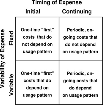
Figure 5.1 Two characterizations, one based on when costs occur and the other on how they vary with usage, result in four categories of costs.

Figure 5.1 shows how these two sets of categorizations – initial, continuing, fixed, and variable - can be combined. This two by two matrix allows planners to identify fixed initial costs, variable initial costs, fixed continuing costs, and variable continuing costs. In this way, costs in studies can be characterized simultaneously by both their relationships to time and how they respond to assumptions about usage.

Sunk Cost

Once a cost has been incurred, even if not entirely paid, it is a “sunk cost.” For example, once a facility has been constructed and is in operation, it is a sunk cost, even if ten years later the company still has its capital depreciation on its books as a cost.

Embedded, Marginal, and Incremental Cost

Embedded cost is that portion of the cost that exists in the current system, configuration, or level of use. Depending on the application, this can include all or portions of the initial fixed cost, and all or parts of the variable costs.

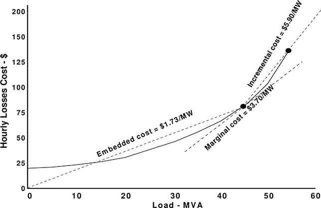
Figure 5.2 Hourly cost of losses for power shipped through a substation transformer as a function of the load. Currently loaded to 45 MVA, it has an “embedded” loss cost of $1.73/MVA, and a marginal cost of losses at that same point of $3.70/MVA. The incremental cost of losses for an increase in load to 55 MVA load is $5.90/MVA.

Often, the “embedded” cost is treated as a fixed cost in subsequent analysis about how cost varies from the current operating point. Marginal cost is the slope (cost per unit) of the cost function at the current operating point (Figure 5.2). This point is usually (but not always) the point at which current embedded cost is defined.

Incremental cost is the cost per unit of a specific jump or increment - for example, the incremental cost of serving an additional 17 MVA from a certain substation or the incremental cost of losses when load on a feeder decreases from 5.3 to 5.0 MVA. Marginal and incremental costs both expresses the rate of change of cost with respect to the base variable, but they can differ because of the inconsistencies and variances in the cost relationships.

In the example shown in Figure 5.2, the marginal cost has a slope (cost per unit change) and an operating point (e.g., 45 MW in Figure 5.2). Incremental cost has a slope and both “from” and “to” operating points (e.g., 45 MVA to 55 MVA in Figure 5.2) or an operating point and an increment (e.g., 45 MW plus 10 MVA increase).

Expenses Now and Then

Almost any electrical project has both initial and continuing costs. Figure 5.3 shows the costs for a new distribution substation, planned to serve 65 MW of residential load on the outskirts of a large city. It has a high initial cost that includes the equipment, land, labor, licenses and permits, and everything else required in building the substation. Thereafter, it has taxes, inspection, maintenance, electrical losses, and other continuing costs on an annual basis. Figure 5.4 shows the initial and continuing costs identified with respect to fixed and variable categories, too. Typical of most electrical planning situations, the initial cost is almost entirely fixed, and the continuing costs are mostly variable.

Decisions Based on When and How Much is Spent

Any utility planner must deal with two types of time versus money decisions. The first involves deciding whether a present expense is justified because it cancels the need for some future expense(s). For example, suppose it has been determined that a new substation must be built in an area of a utility’s service territory where there is much new customer growth. Present needs can be met by completing this new substation with only one 25 MVA transformer, at a total initial cost of $1,000,000. Alternatively, it could be built with two 25 MVA transformers installed, at a cost of $1,400,000. Although not needed immediately, this second transformer will be required within four more years because of continuing growth. If added at that time, it will cost $642,000 extra - $242,000 more than if it is included at the time the substation is first built. The higher cost to add it later is a common fact of life in T&D systems’ planning and operation. It’s also a reflection of the additional start-up cost for a new project and of the higher labor and safety costs required for installing a transformer at an already-energized substation, rather than when the site is cold.

Which plan is best? Should planners recommend that the utility spend $400,000 now to avoid a $642,000 expense four years from now?

A second and related type of time-vs.-money decision is determining if a present expense is justified because it will reduce future operating expenses by some amount. Suppose two types of distributed generators are candidates for installation at a high-reliability customer site. The first, Type A, costs $437,000 installed. It fully satisfies all loading, voltage regulation, and other criteria. On the other hand, the higher efficiency type B unit will also meet these same requirements and criteria and lower annual fuel costs by an estimated $27,000 per year. However, it has an initial cost of $597,000. Are the planners justified in recommending that $160,000 be spent, based on the long-term fuel savings?

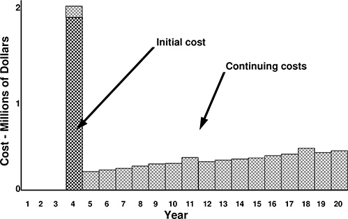
Figure 5.3 A new substation’s costs are broken into two categories here, the initial cost, a one-time cost of creating the new substation, and its continuing annual costs which are required to maintain it in operation.

Figure 5.4 The new substation’s costs can also be viewed as composed of both fixed costs - those that are constant regardless of loading and conditions of its use, and variable costs. Those costs change depending on load, conditions, or other factors in its application as part of the power system. In this example, the variable costs increase nearly every year, reflecting higher losses’ costs as the load served gradually increases due to load growth.

These decisions, and many others in utility planning, involve comparing present costs to future costs, or comparing plans in which a major difference is when money is scheduled to be spent. To make the correct decision, the planner must compare these different costs in time on a sound, balanced basis, consistent with the electric utility’s or DG owner’s goals and financial structure.

Common Sense: Future Money Is Not Worth As Much As Present Money

Few people would happily trade $100 today for a reliable promise of only $100 returned to them a year from now. The fact is that $100 a year from now is not worth as much to them as $100 today. This “deal” would require them to give up the use of their money for a year. Even if they do not believe they will need to spend their $100 in the next year, conditions might change and they might discover later that they do need that money. Then too, there is a risk that they will not be re-paid, no matter how reliable the debtor.

Present Worth Analysis

Present worth analysis is a method of measuring and comparing costs and savings that occur at different times on a consistent and equitable basis for decision-making. It is based on the present worth factor, P, which represents the value of money a year from now in today’s terms. The value of money at any time in the future can be converted to its equivalent present worth as:

Value today of X dollars t years ahead = X × P^t         (5.1)

Where P is the present worth factor

And t indexes the year ahead

For example, suppose that P = .90; then $100 a year from now is considered equal in value to today’s money of

100 × (.90) = $90

and $100 five years from now is worth only

$100 × (.90)5 = $59.05

Present worth dollars are often indicated with the letters PW. Today’s $100 has a value of $100 PW, $100 a year from now is $90 PW, $100 five years from now is $59.05 PW, and so forth.

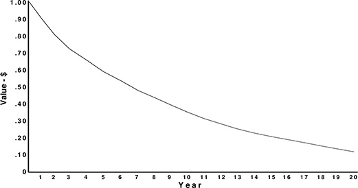
Figure 5.5 Present Worth Analysis discounts the value, or worth, of a dollar the further it lies in the future. Shown here is the value of one dollar as a function of future year, evaluated at a .90 present worth factor (11.1% discount rate).

Alternatively, the present worth factor can be used to determine how much future money equals any amount of current funds. For example, to equal $100 present worth, one year from now a person would need

$100/.90 = $111.11

Two years from now, one would need $100/(.90)² = $123.46 to equal $100 PW.

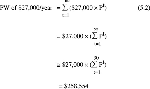
A continuing annual future cost (or savings) can be converted to a present worth by adding together the PW values for all future years. For example, the present worth of the $27,000 in annual fuel savings discussed for the type B DG unit earlier in this chapter can be found by adding together the present worth of $27,000 next year, $27,000 the year after, and so forth

PW of $27,000/year=Σt=1∞($27,000×Pt)=$27,000×(Σt=1∞Pt)≅$27,000×(Σt=130Pt)=$258,554

How Are Present Worth Factors and Discount Rates Determined?

There is no one rule or set of guidelines that rigorously defines what contributes to the present worth factor (PWF), or its companion, the discount rate. Likewise, there is no inviolate formula like Ohm’s law or Schroedinger’s equation that lays out completely and with no exceptions exactly how to compute PWF from those factors that are deemed relevant. Quite simply, PWF is merely a number, a decision-making tool that allows planners to compare future expenses to present ones. The present worth factor is often arrived at through careful analysis and computation, but sometimes it is an empirical estimate “that just works well.”

The present worth factor is simply a value that sums up all the reasons why an organization would prefer to spend money tomorrow rather than today.

There can be many reasons why a person may wish to limit spending today in favor of spending tomorrow. These reasons all influence the selection of a value for the present worth factor. Priorities vary greatly from one company to another and also change with time. Among them is one-reason planners often finding difficult to accept: “We just don’t have the money, period.” In most electric utilities, present worth factors and discount rates are determined by a utility’s financial planners and based on the company’s regulatory requirements for financing and use of money. The methods applied to fix these requirements quantitatively and their relation to PWF are beyond the scope of this discussion, and available in other texts (e.g., IEEE Tutorial on Engineering Economics). However, it is worth looking at some of the primary influences on the present worth factor and how and why they influence it.

Present Worth Factor Is a Decision-Making Tool, Not a Financial Factor

Thus, the present worth factor and discount rates are merely tools. Present worth analysis is a decision-making method to determine when money should be spent. It can embrace some or all of the factors discussed above, as well as others. Two equally prudent planners might pick very different present worth factors, depending on their circumstances, as summarized in Table 5.1 with the inputs that determined the PWFs used in the mid-1990s by a large investor-owned utility (IOU) in the northwestern United States and a municipality in the southwestern United States.

But while the present worth factor can be affected by many factors, the simple fact is that such determinations are irrelevant to the electric service planner. Present worth factor is used to evaluate and rank alternatives based on when they call for expenditures. It is just a tool, part of the analysis, period.

A relatively low PW factor means that the planning process will be more likely to select projects and plans that spend today in order to reduce costs tomorrow. As the PWF is decreased, the planning process becomes increasingly unwilling to spend any earlier than absolutely necessary unless the potential savings are very great. A very low PW factor will select plans that wait “until the last moment” regardless of future costs.

Table 5.1 Discount Rate “Computation” for Two Utilities

Table 5.2 Comparison of Yearly Expenses by Category for an Eight-Year Period

*Taxes and losses for the transformer added in year eight (alternative B) are prorated for that year, since it is assumed here that it is installed just prior to summer peak (six months into the year).

Comprehensive Present Worth Example

Table 5.2 and Figure 5.6 show more cost details on the two-versus-one substation transformer decision mentioned at the beginning of this section. In the case shown, the decision is being made now (in year zero), even though the substation will actually be built three years from now - the decision must be made now due to lead time considerations. Alternative A calls for building the new substation with two 25 MVA transformers at a total cost of $1,400,000 initially. Alternative B defers the second transformer four years (to year 7), reducing the initial cost to $1,000,000. And again, the addition of the second transformer four years later is estimated to cost $642,000 because of project start-up costs, separate filing and regulatory fees, and the fact that the work will have to be done at what will then be an energized site.

However, this decision involves other costs, which while secondary in importance, should be considered in any complete analysis. For example, no-load losses, taxes, and O&M will be greater during the first four years in Alternative A than in Alternative B. Table 5.2 and Figure 5.6 compare the expenditure streams for the eight-year period for both alternatives, including capital; operations, maintenance, and taxes (O&M&T); and losses.⁴

⁴ The table and figure cover the only period during which there are differences that must be analyzed in the decision making. At the end of the eight-year period, the two alternatives are the same – either way the substation exists at that point with two 25 MVA transformers installed. Present worth thereafter is essentially the same.

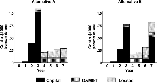
Figure 5.6 Yearly expenses for the two alternative plans for the new substation (constant dollars).

Note also, that the capital for substation construction in either alternative is not spent entirely in the year the substation is completed. A small amount is spent two years earlier (for filing and preparing for the site), and the site, itself, and some equipment purchased a year earlier so that work can begin on schedule.

In comparing differences in the two alternatives, observe also that the second transformer in Alternative A increases O&M&T costs during the first four years of operation as compared to the other alternative, because taxes must be paid on its additional value, and it must be maintained and serviced.

The difference in losses’ costs is more complicated. Initially, losses are higher if two transformers are installed, because this means twice the no-load losses, and the twin transformers are initially very lightly loaded, so that there is no significant savings in load-related losses over having just one transformer. But by year six the two-transformer configuration’s lower impedance (the load is split between both transformers) produces noticeable savings due to reduced losses as compared to the other alternative.

Overall, Alternative A spends fewer dollars in the period examined $142,000 less. It has the lower amount of long-term spending.

Table 5.3 and Figure 5.7 show the various cost streams for both alternatives converted to PW dollars using a present worth factor of .90 (equivalent to p = 11.11%). Note that dollar amounts have dropped– discounted future dollars just aren’t as valuable as the undercounted dollar figures. More important, is the present worth evaluation reverses the order of cost preference for the two options. Even though its total spending is less, Alternative A is rated a higher present worth by $51,000 PW, because many of its expenses are closer to the present.

The total difference in PW is slightly more than 3% of the average PW value of the alternative. Considering the straightforward nature of this analysis, and the high proportion of the various cost elements common to both alternatives, it is very unlikely that the analysis is in error by 3%. Therefore, this is very likely a dependable evaluation: Alternative B is the recommended “low-cost” option. Alternative A would cost more.

Looking at the sensitivity of this decision to present worth factor, the two alternatives would be considered equal if the evaluation had used a present worth factor of .937, equal to a discount rate of 6.77%. Present worth factor would have to be higher (i.e., the discount rate lower) to have reversed the determination that Alternative B is, in fact, the low-cost option.

Again, considering that nominal PWF values less than .92 are extremely uncommon, the recommendation that Alternative B is the preferred option seems quite sound. Therefore, the planner’s recommendation should be to build the substation with one transformer initially, and add the other at a later time, as needed.

Levelized Value

Often, it is useful to compare projects or plans on the basis of their levelized annual cost, even if their actual costs change greatly from one year to the next. This involves finding a constant annual cost whose present worth equals the total present worth of the plan, as illustrated by Figure 5.7. Leveled cost analysis is a particularly useful way of comparing plans when actual costs within each plan vary greatly from year to year over a lengthy period of time, or when the lifetimes of the options being considered are far different. It also has applications in regulated rate determination and financial analysis. In general, the present worth, Q, leveled over the next “n” years is

Leveled value of Q over n years = Q (d × (1+d)ⁿ )/((1+d)ⁿ - 1)         (5.4)

Thus, the steps to find the leveled cost of a project are: 1) Find the present worth of the project and, 2) Apply equation 5.2 to the present worth. As an example here, using Alternative A’s calculated total present worth of $1,684,000 from Table 5.3, that value can be levelized over the seven-year period in the table as

= $1,684,000 (.1111(1.1111)⁷/(1.1111⁷ - 1)

= $358,641

Table 5.3 Comparison of Yearly Present Worth by Category for an Eight-Year Period

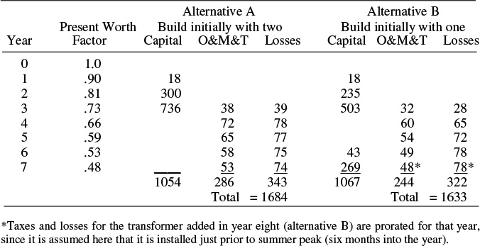
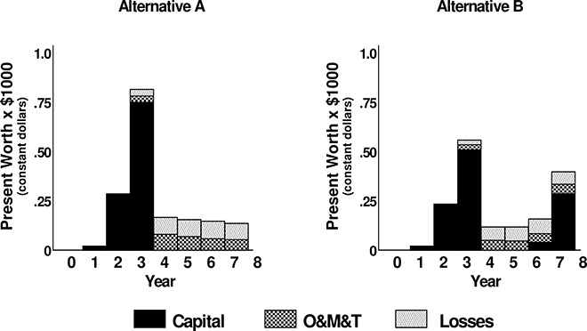
Figure 5.7 Present worth of expenses associated with the two alternative substation plans given in Table 5.2 and Figure 5.6.

By contrast, Alternative B has a levelized cost over the same period of $347,780. If the utility planned to pay for alternative A or B over the course of that seven-year period, the “payments” it would have to make would differ by a little more than $10,800 per year.

Lowest Cost Among Alternatives

In many cases and from many perspectives, the goal of planning is to identify an alternative with the lowest cost. If all pertinent costs (capital, losses, O&M&T, etc.) are considered, and the appropriate type of present worth adjustment is made for timing, lifetimes, and schedules, then the alternative with the lowest PW cost is the preferred option.

Payback Period

The period of time required for “long-term” savings to re-pay the initial investment is often used as a measure of the desirability of making an investment in a resource or other addition to the electric supply. Returning to the “type A versus type B DG unit” problem discussed earlier in this chapter, a fuel savings of $27,000 per year will require six years (6 × $27,000 = $162,000) to repay the $160,000 additional cost of the type B unit over type A. (If the break-even is computed based on PW dollars at a .90 PW factor, the payback of the original $160,000 takes ten years.)

“Payback period” analysis is most often used informally, to provide an additional perspective on plans and financing. Rarely is it part of the formal planning criteria or a specific cost-effectiveness test called for by regulatory authority or management. However, it does address one question that can be quite important to any investor - “When will I get my money back?”

Benefit/Cost Ratio Analysis

In many planning situations, one or all of the options being considered have both costs and benefits, and there are constraints or interrelated considerations with respect to both that impact the selection of the plan. In such cases, planning consists of more than simply ranking the alternatives by cost and selecting the one at the top of the list. Alternatives vary in benefit, too. This situation is particularly common in IRP situations, where options such as DSM have a cost, but also benefits accruing from their use.

Very often in such cases, the planning decisions are based on an evaluation of the expected gain versus the cost. Benefit-cost ratio is a simple concept: a ratio less than one indicates the project will lose more than it gains; the higher the benefit/cost ratio above 1.0, the greater the potential gain relative to its cost. For example, suppose that it has been determined that a particular project, with a PW cost of $160,000, would provide PW savings equal to $258,600. A planner could evaluate the benefit to cost ratio of this proposal as

Benefit/Cost = $258,600/$160,000 = 1.62

This alternative has more benefit than cost - 62% more.

Benefit-cost ratio is generally applied as a ranking method, to prioritize projects that are viewed as discretionary or optional, or in cases where there simply isn’t enough funding for all the projects that present worth analysis has indicated are worthwhile. It has drawbacks, however, as explained below.

MARGINAL BENEFIT/COST ANALYSIS

Example Problem from an Aging Infrastructure System

Table 5.5 shows the different planning options available for two feeders in a utility, which has aging infrastructure problems. Feeder 1 does not currently exist, it is being planned for a growing part of a utility service territory where new customers are developing, customers who must be served in order to meet the utility’s obligation to serve (or a wireco’s obligation to connection). This new distribution feeder can be built in any of several sizes and designs, as shown, using conductors and layouts of various types, all with advantages and disadvantages (including differences in cost). The details of exactly what each alternative is, and the differences in costs are unimportant to this discussion. What matters is that there are alternatives for the construction of this new feeder, and that they differ in both ability to handle future growth without further construction and service quality. Note that “do nothing” is listed as an option. This is not a feasible option for the utility, but for completeness sake it is given a PW cost of $20,000,000 – the consequences, at least in part, of not serving these new customers.

Feeder number 2 is an existing feeder with an average equipment age of 45 years, part of an aging infrastructure area of the system. Slow load growth (.3% per capita increase annually) has exacerbated the usual problems that aging causes, leading to below-average service quality. The table shows the capital costs for various rebuilding programs, along with their expected PW costs based on project O&M savings and restoration costs, calculated by analysis of age, equipment condition, load curves, and failure-likelihood. Again, “do nothing” is an option in this case.

Least-Cost Selection of Alternatives (Traditional Approach)

Traditionally, electric utilities have applied a planning paradigm that includes several fundamental assumptions:

1) All new customers will be connected to the system.

2) All new designs will meet standards.

3) Long-term (e.g., present worth) costs will be minimized.

4) Capital funding for any project that meets the above requirements will be forthcoming.

This paradigm can be labeled an engineering-driven paradigm, because engineering requirements (1 and 2 above) drive the decision-making process (3) and define the financial requirement (4). This is illustrated in Figure 5.9.

In this traditional approach, the two alternatives in Table 5.5 would be evaluated for total present worth cost over a long period (usually 30 years) or alternatively on a lifetime basis, adding together present worth costs for both initial and continuing operating costs over the period. If load projections and planning criteria showed that the feeder had to be upgraded during the period, the present worth cost of the future capital cost for that upgrade would typically be included.

Table 5.5 Two Feeder Project Alternatives Evaluated on the Basis of Least-Cost Present Worth Value System at 11% Discount Rate - $ × 1000

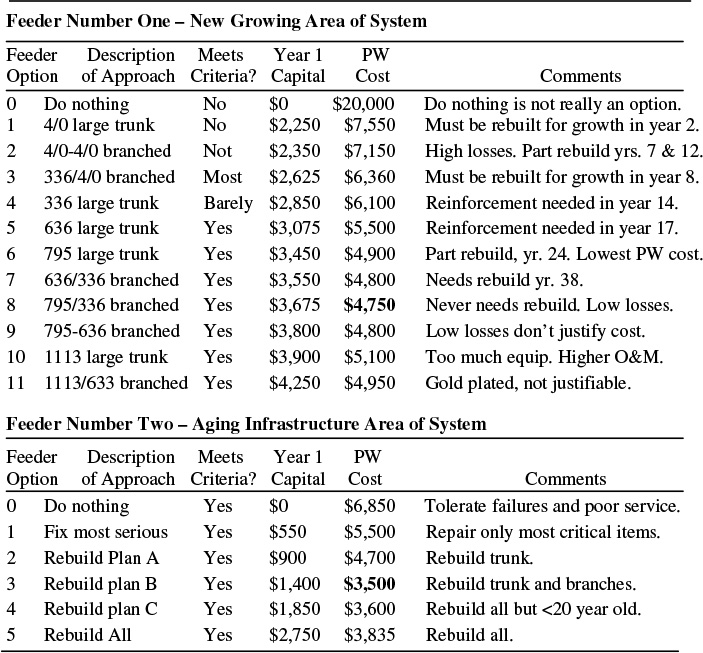
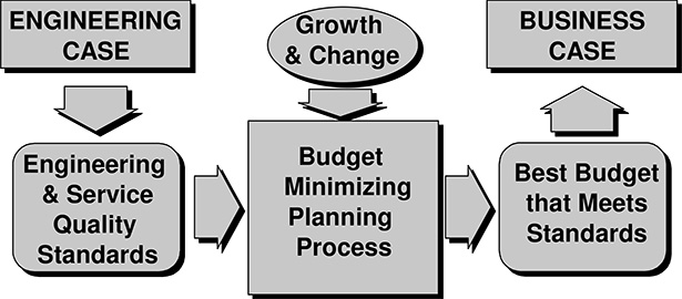
Figure 5.9 The traditional engineering-driven approach to prioritizing projects and determining utility budgets.

In each case, the alternative with the lowest PW cost would be selected. In the example shown in Table 5.5, this process would select option 8 for feeder 1 (the 795/336 branched feeder design) at a capital outlay of $3,695,000 and option 3 for feeder 2 (rebuild plan B) at a cost of $1,400,000. The utility would need a total of $5,075,000 in capital for the two projects, probably borrowing the money for this work, as is the typical financial method at most investor owned utilities.

Facing Budget Constraints

Suppose the utility that needed to do both projects listed in Table 5.5 was forced to reduce its capital budget by 30% in order to achieve financial targets for both rate and stock return reasons. This reduction would drop the $5,075,000 capital total for the two projects to an allowable $3,550,000.

One possible adjustment within the traditional paradigm to accommodate budget constraints is to change the time-value of money used in the PW analysis. The discount rate can be raised to 20%, 30%, or even higher, with the result that it “cuts” items from the approval list of projects. Each increase in discount rate reduces the perceived value of future savings from a project, and biases the decision-making process in favor of alternatives with lower initial costs, such as “doing nothing.”

To achieve the desired reduction to below, $3.55 million in this example, a discount rate 38% is necessary. This will force the selection process for the two example projects to $3,550,000 by selecting only option 7 for feeder 1, and selecting nothing for feeder 2. This provides a total cost of $3.55 million (just meeting the budget) and selects “do nothing” for the refurbishment project.

Using this approach, the capital budget required by the planning process is reduced. However, there are four practical problems with this approach:

1. It does not provide a mechanism to force the budget below any specific limit. By trial and error, the utility can find a discount rate that “works out” to the right budget, but it is not a simple process. More important, it is not a dependable process: next year the required discount could be different. This approach does not lead to a simple rule that can be “aimed” at a specific budget target.

2. No ability to make really difficult cuts. As discussed in Chapter 6, PW analysis never says “no” to essential projects. In the face of severe budget cuts, the traditional paradigm still decrees that all new construction must be done, and work must be done to standards.

3. Using a high discount rate is inappropriate. High discount rates means future savings are unimportant, which is not true: The utility’s current financial situation precludes it from affording long-term savings, but this is not the same as saying it does not want them. (The importance of this distinction will become clear in several more pages.)

4. Customers in older areas of the system might legitimately complain that they are not getting the service and attention they deserve. New customers in outlying areas get shiny new service built to high standards. They get old equipment and lousy service.

Raising the discount rate to accommodate this budget reduction needs to change only the relative importance of the future savings against which present costs are evaluated: The planning method still assumes that the goal is to balance long- and short-term costs. Truly deep budget cuts need to be addressed by looking at how necessary the various projects are today, not at how today’s costs weigh against tomorrow’s savings, in any measure. (This will be discussed at length in a few paragraphs.)

Using Benefit/Cost Ratio to Make the Decisions

Ranking projects based on the benefit/cost ratio is often used to decide among project alternatives. This method can compare the present value of savings over the life of the project to today’s cost to implement. One can also evaluate projects based on their payback period. The two methods usually produce comparable results, selecting or rejecting the same sets of projects. With all proposed projects ranked in this manner, the utility can then determine how much capital it would need to finance all worthwhile projects. Alternatively, it can chose to find only those above any arbitrary benefit/cost limit.

Figure 5.10 plots the results of such analysis for the two feeder projects from Table 5.5, and others that are in the present-year budget. This particular utility needs $88 million to finance all worthwhile projects, as determined by traditional (PW least cost) planning paradigms.

The utility could achieve a budget reduction of 30%, limiting capital spending to only $61.6 million, by approving only projects with a benefit-cost ratio of 4.4:1 or better.

Table 5.6 shows the impact of using benefit cost ratio as the arbiter in prioritizing the two example feeder projects. The benefit cost ratio selected for each option for both projects is shown in the rightmost column. For feeder 1, option 6 is selected (795 large trunk) at $3,450,000. For feeder 2, nothing is selected; all the options fall below the cutoff. The utility would have to have a budget of at least $77 million (only a 12.5% reduction) before any of these projects would be approved.

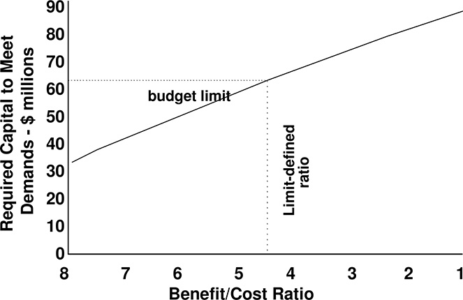
Figure 5.10 Cumulative capital requirements versus benefit/cost ratio for all “worthwhile” projects. The utility needs $88 million. Using B/C as the prioritization test, a reduction of 30% (to $61.6 million) means it can afford projects only up to 4.4:1, and only those with a B/C ratio above that limit should be approved. Benefit/cost ratio provides a way to limit spending to within a severe budget constraint, but it does not spend that budget most effectively (see text).

Table 5.6 The Two Feeder Projects From Table 5.5 Assessed By B/C Ratio

Results Still Not Completely Satisfactory

The use of B/C ratio as the prioritization for projects resulted in only slight real improvement over the use of a higher discount rate. Of the four objections listed earlier for that approach, there still exist numbers 1 and 4:

1. B/C ratio analysis does not provide a mechanism to force the budget below any specific limit. By trial and error, the utility can find a discount rate that “works out” to the right budget, but it is not a simple process. More importantly, it is not a dependable process: next year the required discount could be different. This approach does not lead to a simple rule that can be “aimed” at a specific budget target.

(Objections 2 and 3 were solved by the use of B/C analysis)

2. Customers in older areas of the system might legitimately complain that they are not getting the service and attention they deserve. New customers in outlying areas get shiny new service built to high standards. They get old equipment and lousy service.

Number 4 is a particularly damning objection in the long run, sure to get the utility into trouble with its customer base and regulators alike.

Budget Constrained Planning: Optimization Using Marginal Benefit Cost Ratio

Marginal Benefit Cost Analysis

Table 5.7 shows the options for the two feeders evaluated on a marginal benefit/cost ratio basis. In each project, the additional present worth savings delivered by moving up from one option to the next is evaluated against that additional expense.

Given a budget constraint of $3,550, planners “buy” the most effective use of their dollars by taking the options whose marginal benefit cost ratios are shown in bold (final column) in Table 5.7. This is option 3 for feeder 1 and option 3 for feeder 2. A total of $3,525,000 in expenses for the two projects gains a total savings (over do nothing) of $15,790. No other combination of choices delivers so much “bang” for the buck.

Figure 5.12 shows the budget requirements when all projects the utility is considering are re-ranked on the basis of their marginal present worth/marginal capital ratio. There, the total for every marginal B/C ratio is determined, a plot analogous to that of Figure 5.10 in how it is used, but using marginal rather than just benefit cost ratio. As before, slightly more than $88 million is required to meet all projects with a ratio above zero. As indicated, when limited to $61.6 million, the utility must approve only projects with a MPW/C ratio of 1.5:1 or better. But, unlike the case where it was using benefit/cost ratio as the guiding rule, it will now always “buy” an equivalent ( and biggest overall) PW savings -the most it can afford.

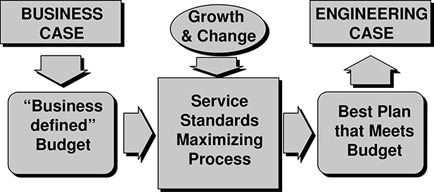
Figure 5.11 Many utilities have shifted to a business-driven structure, in which business needs define the available budget. The traditional planning paradigm has difficulty adjusting to this external change in cases where the reduction from traditional budget levels is significant. Although this paradigm stretches some traditionally rigid standards, it obtains both better reliability and better economy from the limited budget.

Application of Marginal Benefit-Cost Evaluation

Generally, the way one proceeds with the decision making on two or more projects using this approach is shown in Table 5.8. There, the options for the two feeder projects (from Table 5.7) have been merged and sorted into order based on marginal benefit cost ratio. Planners make their selections against a budget total by moving down the table, selecting options and adding their marginal cost (delta cost) into their total, stopping when they have the appropriate budget total (equal to the limit).

Given a budget limit to work within, ($3,550,000 in this example), planning begins by selecting feeder 1 option 1 ($2,250,000), the highest item on the table. It then proceeds to add feeder 1, option 2, for an additional $100,000, as well as option 3 for that same feeder, at $275,000, for a total so far of $2,625,000 in cost. The next item on the list is feeder 2 option 1 with a marginal cost of $550,000, bringing the total spent so far to $3,175. Finally, feeder 2 option 2 can be added, at an additional $350,000, bringing the total to $3,525, the best, with the options listed, totaling under $3,550.

Table 5.7 The Example Two Feeder Projects From Table 5.5 Assessed By Marginal B/C Ratio

Table 5.8 Options for Both Feeder Projects From Table 5.7 Merged Into One List, Ranked By Marginal B/C Ratio

Figure 5.12 Cumulative capital requirements for the utility, versus the marginal PW/capital ratio required for that level of requirement. The utility’s $61.6 million budget allows it to spend up to a 2.1:1 marginal benefit cost ratio. This approach provides a much better guiding rule for project approval and assures maximum overall “bang for the buck” using the limited capital budget.

Pareto Analysis

Pareto Analysis is the basic analytical and decision-support engine of asset management. It is a strengthened version of the budget-constrained approaches discussed in the previous sections. Suppose planners at Big State Electric (BSE) identify 100 major capital spending projects the company could do in the next year, each with a defined scope (what it involves and what it does), an estimated cost, and estimated impacts on corporate KPIs (key performance indicators) like SAIDI, safety, system losses, power quality, working down the age of critical yet old equipment, future profit margins, etc. Taken together, all 100 projects might cost $500 million. However, BSE would never fund all of them, for two reasons. First, it doesn’t have anywhere near $500 million – it is thinking of spending somewhere maybe up to $150 million and might be able to stretch to $200 million if pressed to the wall, but no further. Further, some combinations of these projects don’t make sense if done together. BSE would never refurbish the vaults in its downtown network and replace them, but planners have scoped out potential projects to do both, in order to comprehensively look at the company’s options: they’d like to see them replaced, but things are complicated, there are a lot of other important goals, too, and money is tight. Maybe refurbishment is all BSE can afford. Maybe it can’t even afford that. Asset management will help the planners decide what to recommend.

Portfolios

A portfolio is a combination of projects and programs the utility decides to approve and execute. Traditionally, the utility called the set of projects it approved each year “the capital budget,” a term that stressed what it was spending, or “the approved construction list,” a term that stressed that it was going to build. Calling it a portfolio instead stresses that these projects are investments, i.e., that the company expects something in return and in fact wants to maximize that return. Each circle in Figure 5.13 represents a different potential portfolio, some combination of projects and programs that the utility could decide to fund. The vertical axis is a measure of its contribution to success (how much the utility gets toward its KPI targets) while the horizontal axis is a measure of its cost (how much it spends) for that particular set of projects and programs. Each circle is plotted based on its total “bang” (what it provides in total towards the KPI goals the utility wants) versus “bucks” (what all of its projects cost when added together).

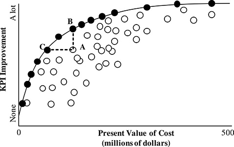
Figure 5.13 Potential portfolios (asset use and spending plans) can be plotted by their cost and performance results as shown here and explained in the text. Only the best portfolios lie on the efficient frontier, also called the Pareto curve, which denotes the maximum performance possible at every budget level. Optimization used in asset management finds only the portfolios on the efficient frontier and draws the curve for the utility planners.

Some of the potential portfolios in Figure 5.13 are inefficient portfolios (unshaded circles). BSE could buy any of these but never will, because it knows it can get more for its money. For example, why fund the combination of projects called portfolio B when one can fund A instead and get roughly 30% more “bang” for the same money? Or the company could fund portfolio C and get the same bang but for considerably less money. Portfolio B is inefficient, whereas A and C are efficient portfolios: if you want as much bang as C gives, you have to spend at least what C costs – no other portfolio can give you that much or more for less money. Similarly, if you want as much as B provides, it is the least costly way to get it.

The efficient frontier is the set of all efficient portfolios, and can be thought of as the upper boundary of this set of portfolios. The efficient frontier represents the set of efficient portfolio choices BSE has with regard to how much performance it wants to buy. This efficient frontier is also known as a Pareto curve, since it identifies a set of optimal solutions based on the same efficiency concepts used by the Italian economist Vilfredo Pareto when he examined issues related to social welfare (Pareto, 1906).

Efficient Choices

A key concept of asset management is efficient choice. The Pareto optimization determines the information shown in Figure 5.13 and identifies the frontier. This gives BSE a set of choices which are all optimum in the sense they maximizing what it gets for the money it spends. But the optimization does not chose or even identify a best plan. The utility executives must do that, deciding how much of one thing they want (money) versus the other (success).

Finding the Pareto curve is straightforward in concept even if technically intricate in practice. The major steps planners have to take to do so are:

1) Define all the projects, their costs, and KPI impacts.

2) Convert the KPI impacts to a single valued measure (benefit).

3) Rate each as to benefit/cost ratio (bang for the buck).

4) Sort them by benefit/cost ratio, highest to lowest.

5) Plot them cumulatively in a figure like that shown in Figure 5.13.

The result is the Pareto curve for this list of potential projects. At each point on the curve, no combination of projects taken from that list can provide more bang for the buck than the combination already plotted: the curve describes the efficient frontier for the utility. The curve has a decreasing slope: initially spending is very efficient, providing a lot of benefit for the money spent, but as more is spent each successive project is, at best, only as efficient as the one before it- the result of sorting them and putting them in order of bang for the buck.

Figure 5.14 shows an actual set of 300 projects, taken from an asset management study for a large investor-owned electric utility in the central United States in 2004. Each project is a represented by a rectangle, of height equal to the benefit it provides and width equal to the project’s cost. The project at the lower left is that project, among all, that has the highest benefit cost ratio.

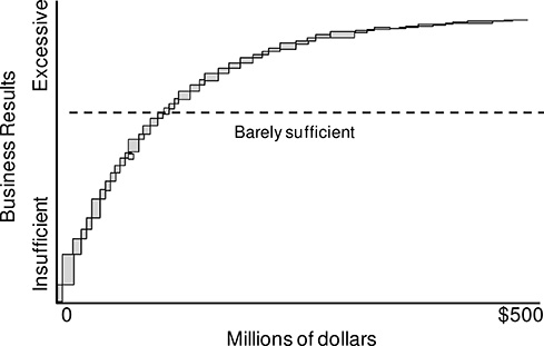
Figure 5.14 Pareto curve representing major capital projects for an electric utility. See text for details.

Realities of Asset Management

Figure 5.15 shows an actual Pareto curve from this same set of projects that includes consideration of several practical considerations that have to be included for the resulting plan to have any practical usefulness to the utility. These are:

Must do projects: a utility has to do some projects it must do. For example, it must do road widening projects to allow the state to build a new, wider highway, etc. It may have agreed to put certain existing lines underground when negotiating a new franchise agreement and rate schedule with a municipality in its service territory, etc. These projects are a given: they will be part of the portfolio.

Dependencies and other constraints. Some projects require another project be done first (Smart reclosers can’t be installed in the Eastwood division until a central control and communication hub is installed in an expanded Distribution Operations Center). Other projects are mutually exclusive (The utility can rebuild a set of breakers or replace them, but would never do both). Planners want both in the list of potential projects to be considered because they provide different amounts of long- and short-term benefit and have different costs. They want the optimization to decide which is best for their company.)

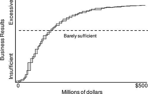
Figure 5.15 The same Pareto curve after practical issues like must-do projects and various practical constraints are considered. Achieving the minimum acceptable level of performance is about 20% more expensive than in Figure 5.14: the real world is just more expensive than theory sometimes estimates. On the other hand, the marginal benefit (slope of the curve = how much one gets for each additional dollar spent above the minimum) at the minimum point is about 25% more than in Figure 5.14. In the real world, the utility has a bit more incentive to spend more than the minimum necessary.

Goals are digital in many practical senses. As a optimization begins buying the best project first, every minute of SAIDI improvement is equally valuable up to the point where enough has been purchased to meet regulatory and business targets for reliability. After that it may not be valuable at all, particularly if other targets like working down equipment age, or reducing O&M costs, or meeting safety goals remain to be achieved.

As a result, the most effective Pareto optimizations never try to combine all the KPI impacts into a single-valued measure. Instead, a multi-target constrained optimization engine is used that is told to find the lowest cost portfolio that:

a) Meets all the minimum targets

b) Includes all must do projects

c) Includes a combination of projects that satisfies all constraints

Asset Management using Pareto Analysis driven by a MIP (mixed integer type) optimization is recommended for utility planning that includes both durability (lifetime and aging issues) and reliability (customer service) as well as other performance and business targets. For more information on utility asset management and optimization of methods see Willis and Brown (2010), which provides an accessible overview or Brown (2012), which gives a very detailed presentation on asset management and methods to implement it, in the References and Bibliography.

Intra-Project, Marginal Benefit-Cost Alternatives Comparison

The foregoing method of maximizing benefit from a limited budget by comparing alternatives within each project (i.e., for each, several alternative ways of doing the project were evaluated) against alternatives from other projects, is called intra-project alternatives analysis. Methods that compare only a single alternative for each project (i.e., the method used in Table 5.5) are called inter-project comparisons. They compare each alternative based only on its ultimate “lowest cost” alternative. By contrast, intra-project comparison ranks the various alternatives for each project against one another.

It is the combination of comparing multiple alternatives in a project, against those of others, and the use of marginal benefit-cost analysis, that yields the additional savings. This method – intra-project comparison based on marginal benefit cost analysis – is called budget-constrained planning, of BCP for short.

BCP is more complicated to implement than traditional prioritization methods. However, the authors have helped several utilities implement it, where it has led to bottom line savings and reliability improvements as dramatic as the improvement shown in the foregoing examples. BCP delivers results. It will be used both in capital planning, and in maintenance and operations prioritization, later in this book. When applied uniformly over an entire utility (all regions, all functions), it is the basis for Results-Driven Management.