
12 Optimization
12.1 INTRODUCTION
In the first edition this chapter was titled Prioritization Methods for O&M and discussed methods for reliability centered maintenance (RCM) of a utility delivery system. The new title reflects a slightly expanded scope. RCM is still covered as before. But the basic prioritization approaches applied in the RCM examples can be set up to work toward maximizing something other than reliability, such as increased lifetime or business value – related but slightly different goals. This chapter discusses the concepts that apply to trying to optimize any goal with respect to service, maintenance, refurbishment, and life extension of power delivery equipment, using RCM as its main example.
The goal of virtually every organization is to try to maximize the results it wants and minimize the consequences it does not. Often this is referred to as optimization. That word, along with its verb, adverb and adjective versions, are often horribly abused terms. Few optimization methods, at least as practically applied, truly find an optimal answer or plan. They find good or pretty good solutions instead, often better ones than a project team can find unaided by such tools. Often other products of optimization’s use are as valuable as the “optimum answer” it provides, products such as the determination of the true cost of constraints and limitations that must be respected, or the interaction effects of various conflicting business goals, etc.
This chapter focuses on methods utilities and industrial power system owners can use to decide how to maximize the care of the power systems they own. Here, “care” means the expenditure of O&M budgets and resources – non-capital resources – on the system, in order to assure that equipment can and will continue to be able to do its job dependably and safely. Regulated utilities are permitted to pass legitimate and approved amounts of O&M expenses on to their customers via the rates they charge for power and energy. However, those O&M budgets are limited to what has been approved by regulators. Beyond that, many utilities and industrial power system owners have only limited numbers of skilled employees and contractors available to do such work, and only limited windows of time during the year when they can do it. For all these reason, a practical reality of power system ownership is that there are always more apparently worthwhile O&M activities that could be done than can be done. Allocation of O&M boils down to priorities – to favoring certain activities like inspection and tracking over more service, or focusing on equipment of a certain age and equipment rather than all equipment, or on only certain types of equipment and not all. This chapter discusses both the function of deciding on how much to fund on what equipment care activities, and why, and analytical and procedural methods used by power system owners to do so. Entire books can and have been written about power system equipment maintenance and service, and provide great detail on techniques as well as the ifs, ands, and buts of maintenance and service applied to different equipment and situations (See References and Bibliography). This chapter focuses on breadth rather than depth, providing an overview with a focus on how the function and the techniques available work toward managing an aging power delivery infrastructure. Section 12.2 begins with some basic concepts about maintenance and service focus and the use of optimization. Sections 12.3 and 12.4 then examine a large (for a textbook) RCM example in a series of evolutions from simplistic to fairly detailed evaluation. Sections 12.5 and 12.6 review several practical issues required to fit technical methodology to a power system’s business needs. Section 12.7 then takes up the concept of optimization, a decision-making process that addresses more than one goal (e.g., reliability and extended equipment lifetime) and considers practical constraints (Project A has to be done before Project B can be done, only one of Projects C, D, or E can be done). The chapter concludes with a summary of key recommendations in Section 12.8.
12.2 PRIORITIZING INSPECTION, MAINTENANCE, AND SERVICE
One Utility: One Decision-Making System
Any utility that wishes to provide good customer service in spite of the challenges created by an aging infrastructure must prioritize its equipment needs and utilize both its physical assets and its O&M resources as effectively as possible. Doing this involves managing three interrelated activities:
1. Prioritization of O&M resources including those for inspection, testing, and diagnostics, along with preventive maintenance, repair, and replacement.
2. Prioritization of capital spending to meet new expansion needs and for replacement of equipment that is too old or costs too much to repair.
3. Utilization of existing and any new equipment, including the loading level for each unit.
Each of these three activities affects how the distribution company utilizes its assets. Each of them interacts with the others: a change in one might change, good or bad, the situation for one or both of the other two. Thus a utility needs to look at how its total budget should be allocated, beginning with whether O&M or capital buys it more performance, while taking all three, and their interactions, into account.
The first two activities spend different parts of the utility’s budget, but each part represents money that is spent. Utility executives and managers must never forget that the third activity – decisions on how to use the equipment – “spends” in a very real way, too. It “uses up” the lifetimes of existing equipment, wearing it out at a faster or slower rate depending on loading, maintenance, and operating policies. Higher loading levels get more value from equipment now, but increase the loss of life rate, “spending” that remaining lifetime faster. Sooner or later, that means both increased O&M costs (as equipment deteriorates from the wear and tear of service, inspection periods must be more frequent, and breakdowns are more common – see Chapters 6 and 11) and higher capital spending (for replacements).
Thus, the power system owner’s goal is to balance all three aspects – O&M, capital spending, and usage, in a way that maximizes the business “value” received for ownership of the equipment, howsoever the organization defines that value. Chapter 15 will present six examples of companies with very different business goals and values and show how those lead to very difference perspectives and guidelines on use, maintenance, and life cycle management.
Prioritization is Needed Because of Limited Budgets
Resources are always limited with regard to what the power system owner would like to do. A utility might have 750 medium voltage breakers in service. It might have data that indicates that inspection and service every three years leads to the fewest problems, best service reliability, and longest lifetimes. But it may have resources, budget, and scheduling windows that permit it to do maintenance and service on no more than 125 years per year. Should it simply cycle through all 750 once every six years? Probably not, if it is trying to minimize customer reliability problems: it can try to focus on units that have an above average effect on customer reliability and an above average need for service - those that have operated more often than most units, or are older and more deteriorated, and are on circuits or in places where they affect the service to large numbers of customers. Regardless, the point is that this question would not arise at all if the utility could do everything and anything it thought necessary: prioritization is needed, and is all about, dispatching or allocating a resource that is scarce – less than all that could be used.
The Need for Prioritization Makes Knowledge of Condition Valuable
A key element of managing an aging infrastructure is condition tracking based on inspection and condition assessment – knowing the level of deterioration and the dependability of specific equipment – so that the infrastructure operator can both decide how best to use that equipment and decide if and how to care for it best. Inspection gathers data that is the basis for that knowledge. By and of itself, inspection and condition tracking do nothing to improve condition, prolong lifetime, or increase the value a utility will see from the equipment it owns. The value they provide is purely in the ability it gives the utility to focus the remainder of its resources – those not spent on inspection but on doing something to the equipment – with greater effectiveness. Thus, a point for all aging infrastructure managers to keep in mind, a key concept behind effective management – is the value of condition knowledge. How much is the knowledge inspection provides worth to the power system owner-operator?
Given that a power system owner has an O&M budget it can allocate to equipment inspection and service of a, how much should it spend on inspection? Spending amount b on inspection leaves only (a-b) for service, but presumably that amount will be more effectively spent because of the knowledge inspection provides.

Figure 12.1 Some amount of inspection and condition tracking will lead to optimum results for the infrastructure owner. This diagram shows a hypothetical situation where 20% of budget spent on inspection doubles the effectiveness of the remaining budget, and spending 80% quadruples it, resulting in 175% and 80% of average results respectively. Spending all monies on inspection results in no benefit.
Thus, the value the power system owners derive from their total inspection and service budget is
Value (a,b) = F(b) x (a-b) (12.1)
where: |
|
a = the total budget |
Function F(b) is an effectiveness of service multiplier that measures how effective the prioritization or targeting of particular items is. It is defined to have a value of 1.0 at b = 0, meaning that the effectiveness at nothing spent on inspection and condition tracking is essentially average: pick the units to maintain at random and over the long haul, the utility will get the average. If an inspection budget b is effective, it might improve results by 10% – F(b) = 10%. If b = 5% to get that 10% improvement in effectiveness, then overall results improve (total result would be 110% x .95 of the budget remaining after inspection expenses, or 104.5%, a 4.5% improvement in results.
In the example of 750 medium voltage breakers above, with no inspection knowledge the owner will select a batch of 125 breakers “at random.” There will be a few in this group that really need service, some that don’t, and many somewhere in between. F(0) = 1.00. The owner gets 125 sectionalizers serviced times 1.0 effectiveness, or 125 units of value from this work.
But suppose the owners spend 20% of the service budget, a, on inspection, so they can bias their selection of units to those that are more in need service. Perhaps the knowledge gained doubles the value they get for every dollar spent on service. But since they spent 20% on inspection they can service only 100 units. Still, they come out a winner: 100 breakers times 2.0 effectiveness = 200 units of value. 1 Spending 20% of a on inspection improved their results by 75%.
If the owners increase the amount they spend on inspection above 20% perhaps they get even more total value. Better inspection leads to more knowledge permits even better dispatching of the service to units where it makes a difference. But at some point, as the monies they devote to service increase, the total value will drop. If they spent all their budget on inspection, it does not matter how effective their service would be because they have no money to spend. Thus, any total-value-derived-versus-amount-spent-on-inspection-curve looks something like that shown in Figure 12.1. It will start off at zero spent on inspection with a value of 1.0. It will rise to some peak value, and then drop to zero and 100%. The owner’s goal is to find that peak value. Knowledge of the function F(b) is the key to optimizing this. Thus, not only does knowledge of condition have value, but so does knowledge of how changing the focus on service changes that value. The case study covered in Chapter 16 will discuss this and how it played out in practical terms for one utility.
1 The authors are deliberately not identifying what effectiveness means here, because this example is, at least on a qualitative level, generalize-able to any and all types of results. Effectiveness could mean the decrease in SAIFI affected by the service, or reduction in unexpected work orders required, or increase in lifetime, etc.
12.3 RELIABILITY-CENTERED MAINTENANCE
A recommended approach to allocation of O&M resources (money, people) for electric utilities faced with aging infrastructure problems is to adopt a form of Reliability-Centered Maintenance (RCM).2 What form of RCM is best depends on details of the utility’s particularly situation. The basic concept is simple: allocate maintenance resources based on how they contribute to reliability.
Maintenance and Maintenance Management
The traditional view of maintenance’s purpose is that it is used:
• To make certain equipment performs its intended function in a satisfactory manner
• To reduce long-term costs by servicing equipment before deterioration causes any avoidable damage
• To avoid unexpected outages by detecting failure in advance
Resources can be allocated by a utility to activities aimed at achieving any and all of these goals (inspection, testing, service, repair). There are several “philosophies” or perspectives on how maintenance can be managed.
1. By the book – do maintenance on a periodic basis. The period between service and the maintenance to be done are exactly as prescribed by manufacturer’s recommendations or applicable standards.
2. By the book (modified) – do maintenance on a periodic basis. To reduce cost, the period between service work and the actual work done each time are respectively the lengthiest period and the leanest amount of service the manufacturer/standards will permit.
3. Only as needed – maintain equipment only when it gives operational signs of needing service (e.g., tap changer non-operative).
4. Reliability-Centered Maintenance. Allocate maintenance resources among equipment in a manner that will maximize the improvement in “reliability.”
2 The authors will use “RDM, to denote results-driven management, which encompasses the intra-project, marginal benefit-cost methods described here (see pages 179-180) applied to both maintenance and capital spending, and the more commonly seen all-caps designation, RCM, for “Reliability-Centered Management, which will mean here the expanded version of RCM described in this chapter.
5. Asset Management. Allocation maintenance resources in an optimized way, taking into account all options and aiming to satisfy multiple corporate goals or targets, and perhaps while also considering the capital budget, as well.
Among utilities in the United States, most traditionally adopted a maintenance program that was somewhere between 1 and 2, performing all the prescribed maintenance on equipment, but often on a slightly less frequent basis than the manufacturers would recommend.
During the 1990s, as electric utilities throughout the United States. faced both increasing competition and uncertainty as to cost-recovery rules in the future, many made every effort to cut spending, including cutting back on maintenance budgets. As a result, there was a shift from (1) above toward (2), with some utilities adopting procedures that were very close to (3), essentially performing maintenance only when equipment failed or gave signs of imminent failure.
Always: A Budget-Constrained Situation
A point worth reiterating is that nearly every modern distribution utility, and certainly every aging infrastructure utility, is permanently in a “budget constrained” situation – there will always be more worthy, and justifiable, uses for resources than there are resources. A modern electric utility simply cannot afford to replace all of its aging equipment just because that equipment is old. It does not have enough funds. Therefore, the number of potential projects (capital) or programs (O&M) that are worth funding will always exceed the number that can be approved. The utility will permanently find itself in a “budget-constrained” situation, where it must make decisions between worthy projects on the basis of “bang for the buck.”
Prioritization for utilities in this situation is about much more than deciding on the order in which projects will be done. It is about deciding which projects will be done, and which won’t be done at all, even though those projects may be worthy and, in some sense (perhaps the traditional sense), justifiable. Prioritization in a budget-constrained situation means determining which projects and programs are the most worthy – which will do the most good – and funding only those with the limited budget.
Techniques to apply that concept to capital projects and to non-maintenance related operating costs are covered in parts of Chapters 5 and given in the case studies covered in later chapters and the Appendices. That same basic concept is used in this chapter with respect to maintenance. All projects, and all alternatives for all projects, are evaluated with respect to how well they help improve customer service quality. Those that provide enough “bang for the buck” are approved. Those that don’t are not.

Figure 12.2 Reliability-centered maintenance does not seek to balance service quality and cost (top), although management practices used to administer it and similar marginal benefit-cost based programs may (see Chapter 15). Instead, RCM seeks to maximize bang for the buck from O&M dollars, which it does by identifying inequalities in what various potential projects and programs will provide for the dollar (bottom).
Reliability-Centered Maintenance
As mentioned above, the real question in allocating resources when faced with service quality challenges is how much will each activity contribute to the utility’s goals, and at what cost? In RCM, the costs of various inspection, testing, service, repair, and replacement activities that the utility could do are assessed on the basis of how much they will contribute to the utility’s goal (good customer service) versus their cost – a merit score. They are then ranked by merit score. Winners are those that score particularly high on a “bang for the buck” basis – those that provide more customer service quality improvement for less money.
Figure 12.2 illustrates this concept. RCM is depicted at the bottom of the figure. Basically, RCM involves weighing the merits of various projects and picking those with the greatest benefit at the least cost. Figure 12.2 also illustrates what RCM isn’t. It is not, as shown at the top, an attempt to “balance” or optimize the total amount of maintenance budget against the value of the resulting service – so called Value-Based Maintenance (VBM). VBM has a place in the planning and decision making at an aging infrastructure utility, but that place is as a strategic planning tool to determine overall budget, and to prioritize the total maintenance budget versus capital and other operating budgets.
RCM Prioritizes Candidate Programs and Projects
RCM prioritizes a group of projects or programs based on merit score, permitting the utility to select the most effective candidates to achieve its goals. Four important points are that:
1. RCM effectiveness is usually determined by both the number of customers served and by the improvement in reliability that is expected from the project (customers x reduction in outage) or something similar.
2. Cost is the total cost of the service or maintenance program, including materials, labor, etc. A key element of good RCM programs is that costs are consistently treated among all classes of equipment and types of activities.
3. Cost may include a credit for avoided costs down the road, such as the avoided cost to repair a failure in the future, suitably discounted for time value of money and any lack of certainty.
4. Benefits do not last forever. Good methods recognize that if a breaker is maintained, it will be in “good shape” for only a period of time, after which it will again need service.
Projects are then ranked on the basis of bang for the buck and the most effective one picked. Working down such a list, a utility chooses all it can afford until it reaches a point where its maintenance budget is exhausted. The remaining projects on the list are not funded.
12.4 BASIC RELIABILITY-CENTERED PRIORITIZATION
Table 12.1 lists 35 distribution system maintenance projects or programs that cover a range of typical maintenance activities.3 These include both major maintenance projects on “large equipment” and smaller projects, as well as a major program (pole inspection/replacement). The entire list of 35 projects has a cost of $3,174,500. However, for this example, the utility has only about 40% of this, or $1,375,000, to spend. It must select the best $1,375,000 worth of projects from out of that list.
These projects could be prioritized in any number of ways, but in this example they will be ranked on the basis of impact on customer service quality per dollar. Impact is the decrease in customer-minutes out of service that is expected from each project during the next few years, defined as
Impact = ΣRt x Pt
Where Rt = reduction in customer minutes out of service per year, in year t, expected due to the activity
And Pt = present worth factor for year t, t = 0 (this year), and years 1, 2, 3 and further into the future
The impact must be evaluated over multiple years, because maintenance projects have a positive impact on equipment reliability that lasts more than one year. This sum usually needs to be evaluated over only the short term, for the next three to seven years. Three years is used in this example, mainly because the tables would become unwieldy if more years of impact improvement were displayed. However, in actual implementation, decisions comparing replacement versus maintenance often need to take a longer perspective, as will be demonstrated with examples given later in this chapter. The concept and method of implementation are identical, however.
Present worth factor is applied to customer outage reductions in future years, in order to adjust all factors onto a present-time basis for the current year. In this case a factor of .9 is used.
Cost in this example is total cost of the proposed activity. In all cases in this example (at least for now), the costs are operating budget items within the present year (year 0), and so no present worth adjustment or consideration of costs beyond the present year needs to be done. Programs or projects that include a continuing cost for several years or a commitment to future expenses, or that make partial payment today with future payment of the remainder for some service or replacement done next year or thereafter, must all be reevaluated with
3 This is literally a “textbook example” created by the authors to illustrate well certain key concepts in RCM. However, all of the data given is both consistent with the authors’ experience in actual utility systems, and with the failures rates, repair costs, and expected improvements given in the various equipment-specific appendices in the IEEE Gold Book (IEEE Recommended Practices for the Design of Reliable Industrial and Commercial Power Systems) and its references.
Table 12.1 Example List Of Projects As Evaluated By RCM Ranking

Table 12.2 Example List Of Projects With Change in Failure Rates for the Next Three Years (%/yr.) Without and With the Proposed Work Being Done

a present worth evaluation of cost. Cost is defined on the same present worth basis as benefits, as
Cost of project i = Costi = ΣCi,t x Pt (12.3)
Where Ci,t = cost of project i in year t
And Pt = present worth factor for year t
Reduction in failure rate due to maintenance
Table 12.2 shows the 35 projects listed with their new failure rates, and present and expected outage rates for the next three years with and without the proposed project performed. The failure rates used here are within the typical ranges seen for distribution equipment in various stages of aging.
This example illustrates one highly recommended procedure. The improvements made in failure rate for each project are defined using a formalized method of estimating improvement (in this case a probabilistic method discussed later in this chapter). It involves classifying maintenance into categories, with each category modeled as having a certain expected impact. 4 Such an institutionalized set of standardized expectations for improvement assures uniformity of purpose and that no one “cheats” the system by using their own maintenance efficacy figures. Categories used here are the following:
1. Complete rebuild returns failure rate to a failure rate equal to “as new condition” plus 5% of the degradation expected over thirty years. Thus, if a new transformer (but one past its infant mortality times) has an annual failure rate of .05%, and a thirty-year-old one has a failure rate of 2.7%, then a recently rebuilt one has an expected failure rate of .05% + .5 x 2.2% = .61%/year.
2. Full service done on the unit cuts the amount of degradation of the equipment by two-thirds. As an example, suppose that a HV breaker has a new failure rate of .92%/year, whereas one badly in need of full servicing has an annual failure rate of 3%. Then, a recently serviced unit has a failure rate of .92 + .33 x (3.00-.92) = 1.61%.
3. Inspection and all repairs found to be needed made cuts failure rate by 40%. This, if a group of old low-voltage breakers, all in need of servicing, has an average expected annual failure rate of 3.5%, but only .056% when new, then inspection and needed repairs reduces the value to an expected annual failure rate of .56 + .60 x (3.5 -.56) = 2.3%.
The above are rough rules of thumb used for this example only and not recommended as hard and fast rules the reader should apply to any utility system.
4 “Expected” here means in a probabilistic sense. Failure is a random process that is best modeled probabilistically. So is improvement.
They illustrate that repair activities have been classified by expected improvement on a category or equipment class basis. No attempt is made to determine what the improvement made by a specific type of service on a specific device would be. Such categorization is highly recommended. Repair and improvements, like failure rates themselves, are probabilistic in nature. Both the concepts of failure rate itself, and failure rate improvement, are probabilistic, and their application works well only when used as probabilistic expectations applied to large sets of equipment.
Obtaining Failure-Rate Reduction Data
A concern for any utility maintenance management team will be “where do we find the data on failure rate reductions for various maintenance functions?” Ideally, these data should be developed by the utility specifically for its situation, or at least based on studies done elsewhere with judgmental adjustment for any unique factors for the utility’s situation.
This is not as difficult as it seems to many. Data is available at most utilities, and if not, then “generic” data based on published and available public domain data, such as that included in various IEEE books and publications, can be used as a starting point. The authors have never seen a situation where the appropriate data cannot be developed to the point where the RCM approach can be applied in a dependable manner.
One strong recommendation is to never use a lack of data as an excuse not to take this approach. In the author’s experience, that is most often used an excuse by people who simply want to continue to do things as they have always been done. If a utility cannot develop a set of reasonable estimates of the impact maintenance makes on its equipment, on a broad category basis as required here, then it is basically admitting it has no idea of the value of the maintenance it is performing. Doing anything whose value cannot be estimated, in the present industry environment, is as extremely imprudent. A utility that does not develop failure rate reduction data has only a very weak basis upon which to justify its maintenance expenses.
Prioritization Based on Ranking
Table 12.3 shows the result of applying the formulas given earlier to the data on the 35 projects shown in Tables 12.1 and 12.2. There, the customer minutes of improvement per year for years zero, one and two is computed and a present worth sum formed. This is then divided by cost to obtain reduction in customer service minutes expected per dollar – “bang for the buck.”
The projects are listed in Table 12.3 in descending order according to their merit score (improvement per dollar), given in the leftmost column. The “bang/buck ratio” for projects on this list varies from a high of 12.84 to a low of 0.01. Figure 12.3 plots the merit score (bang/buck ratio) versus total budget required to buy all projects of that score or better, for this set of 30 projects. For example, the top project on the list (merit score 12.84, has a cost of $27,000). The utility can buy all projects with scores of 12.84 for $27,000. The next project on the list has a score of 11.89 and costs $11,000. The utility can buy all projects with scores of 11.89 and better for $38,000. And so forth. The first eight projects together total only $168,000 – just 5% of the total list’s cost – but provide over 25% of the total improvement in reliability from the entire list.
Table 12.3 Projects Evaluated By RCM Ranking, Listed in Descending Order of Merit
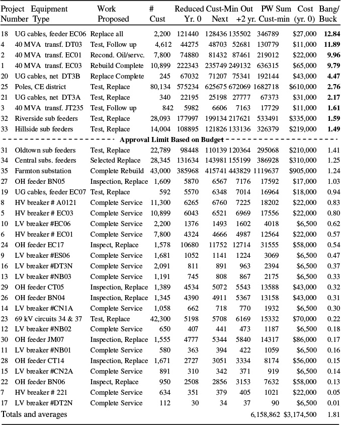
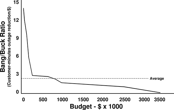
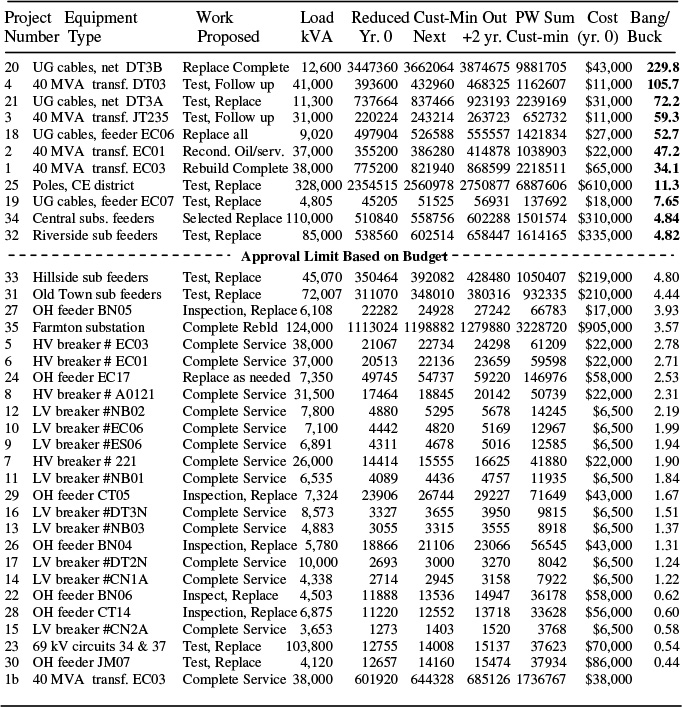
Figure 12.3 Merit scores of projects versus cumulative budget required to buy down to that level. This set of projects exhibits the “scree pattern” typical of many RCM prioritization results. There are a very few extremely high scoring projects (above 3), a number of “pretty good” (3 – 1.5) projects, and a host of projects with lesser merit.

Figure 12.4 Total “bang” that can be purchased versus budget. By selecting the top ranked projects, the utility can buy over two-thirds of the total benefit available for its budget limit of only 40% of the total cost (dotted line).
The plot has a “scree” bend, a sharp change in slope between a few very worthy projects and a large number of others.5 Here it occurs at a budget value of about $250,000. This is typical. Most evaluations of this type are dominated by a few very high-scoring projects, amidst a plethora of others.
Figure 12.5 plots total benefit purchased versus budget. It shows how much money is required to buy what total level of improvement. The cost of the first ten projects in Table 12.3 (those with bang/buck values shown in bold) is $1,374,000, exactly $1,000 less than the allowed budget total in this example. The utility can spend its budget on these projects – only 43% of that needed for the entire list – and receive 68% of the total benefit in customer-minute reductions of the entire list (4,152,729 customer minutes avoided out of 6,158,862 customer minutes possible from the entire list). The “cutoff value” for funding at the $1,375,000 budget limit is 1.49-customer service minutes per dollar. No other set of projects it can afford will attain as much improvement.
What This Prioritization Accomplished
RCM prioritized the proposed projects in a way that permitted the utility to rank and select projects that would use budget-dollars most effectively. Among the projects listed, no other subset will provide more value, assuming the utility’s goal is to reduce customer minutes of outage, than those ranked highest on the list. For any budget limit, the utility merely has to begin selected projects from the top, working its way down the list until it exhausts ist budget.
RCM, then, is basically a tool to help maximize reliability-related operating activities against a budget limit.
Changing the Figure of Merit
RCM does create one conundrum for a utility. It must choose a figure of merit – a particular performance factor to minimize – in this case the expected customer-minutes of outage. Clearly, that choice will greatly affect just what projects are selected, and what benefits the utility “buys” with its maintenance budget.
Continuing with this same example, what if the utility had selected minimization of kVA-minutes of outage, not customer-minutes of outage, as its goal for prioritization? There is considerable merit in using kVA-minutes as the decision-making criterion in RCM. Often, a circuit or transformer will serve only a small number of customers, but those customers each buy a lot of power, and spend a good deal more on power than customers who buy less. One can argue that every kilowatt these larger customers buy should be treated the same with respect to attention and quality control, as those bought by smaller customers. Further, some of these large consumers may be “more important” in terms of societal outage impact.6
5 Scree is a geologic term for the pile of rocks and debris at the foot of a volcanic cinder cone or other tall “monument” rock feature (e.g. Shiprock, NM). As a hard rock cinder cone weathers, bits of rock break away and tumble down to ground level, often rolling some distance from the cone’s near vertical face, and creating the scree – a wide, nearly flat mound surrounding the near-vertical rock monument.
Table 12.4 Projects Evaluated By kVA-Minutes, Listed in Descending Order of Merit
6 Opinion in many parts of the industry holds that interruption of service in the central core of cities and key municipal facilities is much more unfavorable than outages to most other loads, partly due to the impact such outages have on the function of society as a whole.
For example, Table 12.1 showed that project 19 (UG cables, feeder EC07 – test and replace as found necessary) had only 592 customers, about one quarter of the customer count on most feeders, but served 4805 kVA peak load, rather typical for a feeder. Clearly, it serves customers who have a higher demand than average. As a result of the relatively low customer cost, the evaluation shown in Table 12.3 put it mid-pack in the table – it is not to be funded this year. Service to those larger customers will suffer, and for that matter, service to smaller customers on that feeder could suffer in comparison to customers elsewhere.7
Table 12.4 lists the 35 projects re-evaluated and prioritized on the basis of kVA-minutes of outage reduction expected per dollar, rather than customer minutes as done earlier. The values are much different since they are based on a different measure. They vary from a high of 229.8 to a low of .44. Again, the ranking exhibits a scree-like shape (not shown). The utility’s available budget is reached somewhere in the 12th project (approval of 11 leaves it with about $225,000 left, approval of project 12 spends about $100,000 too much. Assuming the first 11 projects are approved and the remaining budget is spent on part of project 12 with proportionate results (it involves many feeders so it would be feasible to only do a portion of it), the total budget of $1,375,000 buys 22,273,339 MVA minutes of reduction, or 64% of the possible reduction. Project 19, the feeder with few but larger-than-average customers, just barely makes the cut, for although it moves up greatly in relative score, a number of other projects do, too. Other changes are approval of Project 34, which did not make the approval list in Table 12.3, and non-approval of Project 31, which falls off the approval list.
The top projects will be at the top of just about any list
While the change in figure-of-merit altered the composition of the approval list, eight of the top eleven projects stayed the same regardless of the prioritization scheme. Looked at another way, in this example 84% of the budget is spent on the projects that make it into both lists.
This is often the case - the very top rated projects stay top rated even if the exact definition of “merit” is changed. The reason is that projects that tend to score extremely high generally do so because they provide a tremendous improvement in equipment reliability per dollar. Whether serving many customers or a high load, that large increase in equipment reliability pays off with a handsome increase in merit score. Careful examination of Tables 12.1 through 12.4 will show that the winners here are all projects where a correction from “very poor” to “very good” reliability is made at a good price. Another way to look at it is that prioritizing on the basis of kVA minutes gains 90% of the optimum result from the standpoint of optimizing for customer-minutes.
7 In actual fact feeder EC07 (#7 out of East City substation) serves three customers of roughly 1 MVA peak demand each and 499 typical small residential and commercial consumers. Had this feeder, which has very severe reliability problems, served only residential and small commercial customers of the same total peak demand (about 1,700 of them would be typical) the higher customer count would have led to a figure of merit of 2.71, putting the feeder on the approval list. As a result, one can argue that these 499 customers were “screwed” just because they happened to be on a feeder serving several large consumers and therefore having a low customer count.
Table 12.5 Comparison of Top Projects

Both merit indices used above were duration-related. Had a frequency of outage index been used, such as customer interruption count, or kVA-interruptions, the results would have been somewhat less similar to those in Tables 12.3 and 12.4. But even so, more than two-thirds of the projects at the top of the list would remain the same even if a frequency-related merit score (e.g., SAIFI) were used In general, the use of any reasonable reliability definition seems to gain at least two-thirds of “optimality” as judged by any other figure of merit. Qualitatively, this is a general result:
The use of any reasonable definition of “merit” as the prioritizing index in RCM will provide qualitatively similar overall results.
What “Reliability Definition” Should A Utility Select?
The answer is quite simple: whatever index its regulatory authority has indicated will be used to evaluate performance of the utility. Generally, that is some combination of SAIDI, SAIFI, and a measure of “outliers” – customers who have much worse than average reliability.8 Regardless, if law or regulation defines “what is important,” the utility would be imprudent to pick anything else, particularly if performance incentives or rate penalties are linked to its performance as assessed by that measure.
8 Most utility regulatory commissions have some provision in their regulations requiring attention to customers/feeder who have much worse (e.g., three times) than average duration or frequency of outages, or who are perennially on the list of worse performance every year.
This is where performance based rates (PBR) provide a great advantage to the utility. PBR not only provides a completely unambiguous definition of what “good performance” means, but it provides a quantitative measure of how much it is worth. This permits not only prioritization of projects as shown here, but optimization of the total budget as will be discussed in Chapter 15.
With very few exceptions, there are no significant problems applying the methods discussed above to any type of regulatory definition of “good performance” or PBR rate schedule. The examples given here are a bit simpler to execute and display on textbook pages, than what is generally required in the most actual utility cases, but the concepts are the identical and the execution requires nothing not shown here. Non-linearities in PBR functions (see Chapter 14, Figures 14.6 and 14.8) create some challenges in analyzing individual projects and prioritizing a list to a budget constraint, but the authors have never encountered any system that cannot be optimized in the manner discussed above.
12.5 PRIORITIZATION OF THE TYPE OF MAINTENANCE
Section 12.3’s RCM prioritized projects by picking from a list of proposed maintenance projects. Projects were prioritized based upon:
• The expected reliability improvement,
• The number of customers, the load, or other measures of importance of the equipment’s service, and
• Cost.
Projects were ranked so that the best can be selected against either a goal of using a constrained monetary budget most effectively (as in the example) or against a goal of achieving some target reliability improvement at the lowest cost possible. Applied with good data, focus on objectives, consistency and common sense, that basic method provides good results. However, results can be improved.
The improvement is based on letting RCM determine what and how much maintenance should be done to each unit. In Section 12.3, each item on the list had a specific maintenance activity (e.g., full rebuild, inspect and replace as needed, etc.) already assigned to it. Prioritization the picks the best breaker-service activities to fund. But overall “bang-for-the-buck” can be improved beyond this, if the RCM method is used to also decide what activity should be done to each breaker, too. Maybe one unit should receive full service, and a second breaker just a quick servicing of only critical components: the money saved there can pay for similar service on another breaker, providing more benefit than if that second breaker were fully serviced.
Table 12.6 Project 8 and Two Alternatives

Table 12.7 Project 8 and Two Alternatives Listed As Marginal Project Decisions
Project |
Equipment |
Work |
# |
Reduced Cust-Min |
Out |
PW Sum |
Cost |
"Bang/ |
|
Number |
Type |
Proposed |
Cust |
Yr. 0 |
Next |
+2 yr. |
Cust-min |
(yr. 0) |
Buck" |
- |
HV breaker # A0121 |
Do Nothing |
11,300 |
0 |
0 |
0 |
0 |
0 |
- |
8c |
HV breaker # A0121 |
Test, Replace |
11,300 |
3797 |
4231 |
4612 |
11340 |
6750 |
1.68 |
8b HV breaker # A0121 |
Partial Service |
11,300 |
949 |
973 |
1005 |
2639 |
2250 |
1.17 |
|
8 HV breaker # A0121 |
Complete Service |
11,300 |
1519 |
1557 |
1608 |
4222 |
13000 |
0.32 |
|
Half Measures Sometimes Deliver More than One-Half the Results
Application of “intra-project” alternatives evaluation
Table 12.6 lists Project 8, from Table 12.1, which was the complete service on a HV breaker #AO121, along with two other alternative categories of service that are possible for that unit - different types of service on that same breaker. These are option 8b, “partial service,” and option 8c, “test and replace as found needed.” The table shows data equivalent to that shown in Table 12.3 for all three alternatives (i.e., the evaluation done against customer outage minutes). Both Options 8b and 8c provide less reliability improvement than the original project proposed, but they also have a lower cost. They provide more “bang for the buck.” Their figures of merit (right-most column in Table 12.6) indicate that unlike the original project (complete service) both 8b and 8c score high enough to have gained approval in Table 12.3 (the selection limit was 1.49).
Table 12.7 lists these two projects in a slightly different way. First, they are listed in order of increasing cost. Secondly for completeness, “do nothing” is listed as an option. Thus, do nothing (the least expensive) is listed at the top. The next line gives Project 8c, along with its costs and benefits, then 8b is listed, and finally 8.
Most importantly, the costs and benefits of each option have been computed as marginal differences. The least cost project (8c) is listed with its costs and reliability improvements as it was in Table 12.6. But project 8b, the next least costly, is listed with marginal costs and benefits. The cost shown is its cost over and above 8c’s. The improvements shown are its improvements minus those that 8c would deliver. Similarly, the original project’s reliability improvements and cost have been converted to the marginal differences that choosing that alternative over 8b would reveal.
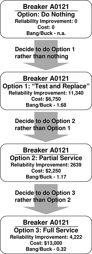
Figure 12.5 The three possible projects for Breaker A0121, viewed as marginal decisions. This is intra-project evaluation – comparison of project alternatives that all fall within one equipment unit or set of equipment – as opposed to inter-project comparison – comparing projects applied to one unit of equipment to those on others.
This marginal benefit and cost table has converted the list of possible projects into a decision chain. It tells the utility what it gets for what it has to pay when it picks any option over a less expensive option. Table 12.7 lists the three projects and “do nothing” as a serial decision chain. This is illustrated in Figure 12.5. These projects are now decisions among different categories of service for the same breaker, a chain of increasingly expensive projects, each providing more reliability improvement than the preceding, but at higher cost.
While viewing a set of possible alternative projects in this manner may seem obtuse, and of no practical value, when dealing with an optimization method as described here, it provides a big improvement. The “chain” of options shown in Figure 12.5 basically reduces a decision with multiple outcomes (which of four alternatives do I choose?) to a series of binary (yes-no) decisions. It simplifies performing the decision-making process with a formal (i.e., rigorous, repeatable, documentable, defendable) procedure that essentially performs a series of binary evaluations (this is better than that). It also illustrates a key point. Doing nothing should always be the basis for comparison: all activities should justify themselves against a “zero base.”
Looking at Table 12.7, note that the scores for these three options (last column), the lowest cost option, 8c has the same as it did in Table 12.6 – a score of 1.68 ($11,340 customer minutes expected reduction over $6,750). But option 8b has a score of only 1.17, rather than 1.55 as evaluated in Table 12.6. While Project 8b looks good enough when viewed on its own, viewed as a decision to spend $2,250 more than Option 8c to gain the improvement it gives over 8c, it does not look quite as good – definitely not good enough to gain approval in Table 12.3. That $2,250 is not nearly as effective in improving reliability as the $6,750 spent on only buying Option 8c. Similarly, when viewed as a marginal option, Option 8 itself looks very inefficient, with a score of only .32.
Table 12.8 shows the RCM evaluation and ranking of all projects from Table 12.3 with these three projects substituted for Project 8. Note that 8c, with its figure of merit score of 1.68, makes it into the “winners” category. Projects 8b and 8 fall far below the approval limit – their additional cost over 8c is definitely not justifiable based on their additional benefit. The recommended action, then, is to select to perform only “testing and replacement as found needed” on this breaker.
What got bumped off the list to make room for project 8b? In this case, nothing. Instead, whereas originally the utility could just afford to buy the top ten projects, it can now not quite afford to buy all of the final projects on the approval list (#32, Hillside substation feeders - testing and replacement as found needed). By the time it gets down to that item in Table 12.8, it is $6,7500 short of having enough to fund this project completely. Prorating that project by assuming that some small portion could be deleted with proportional impact on results, indicates that this change in using alternatives for Project 8 results in a .03% improvement overall.
Using the approval limit’s marginal cost of reliability ($1.41/customer minute) the additional reliability wrought by this improvement over the results of
Table 12.3 would cost the utility another $859 to buy if it stuck to the method used in Table 12.3.
This small improvement may hardly seem worth the effort. However, the point was to introduce the concept of extending the RCM evaluation to deciding how to maintain each unit of equipment, not just what gets maintained. By evaluating options in this manner – letting the RCM decide what is done to what equipment, the total benefit obtained from the spending is improved. As will be shown later, the resulting savings can be significant.
Table 12.8 Projects Evaluated By RCM Ranking, Including Two Options for Project 8
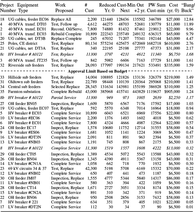
Table 12.9 Projects 1 and 35 with Multiple Alternatives

Intra- versus inter- project alternatives evaluation
Tables 12.6 – 8 showed one example of letting RCM determine what should be done to a unit of equipment. The earlier “optimizations” – those carried out in Section 12.3 – basically decided only among projects where it had already been decided what would be done to each unit. Comparison like that, where decisions about what maintenance will be done has already been made, is called Inter-Project Alternatives Evaluation. By contrast, evaluating the possible maintenance options on one unit of equipment to the possible maintenance options on other units is termed Intra-Project Alternatives Evaluation. It applies the optimization to a broader range of options and thus provides an improvement.
Comprehensive Example Using Intra-Project Optimization
Table 12.9 lists three alternatives to Project 1 and four for Project 35 – the original and two and three alternatives respectively, for each. Also shown is one example of splitting the nine LV breaker projects (numbers 9 through 17 in Table 12.1) into two alternatives. In the original list (Table 12.1, optimized in Table 12.3), nine LV breakers were listed for “full service” at $6,500 each. Here, an option – inspect and replace (as found needed) - is an alternative at only $1,100 in cost but with less effective reliability improvement. All of these options are shown figured as marginal costs and marginal improvements and grouped together as sets of ordered, marginal decisions.
Table 12.10 Projects Evaluated By RCM Ranking Using “Intra-Project” Alternative Evaluation for Twelve Projects (#s 1, 8, 9-17, and 35).
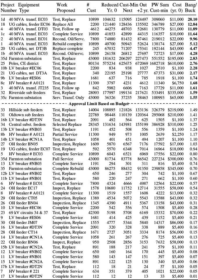
A different set of decisions
Table 12.10 shows the result of an RCM ranking based on customer-minutes that includes these alternatives added to the projects and alternatives used in Table 12.8 (including Project 8’s options). Among the first eight projects at the top of the list are all four of the alternatives to Project 1. Although the RCM method had a list of partial measures it could consider for this unit, it chose to “fully upgrade” Project number 1 through selection of its alternatives 1d, then 1c, then 1b, to 1. Thus, for that transformer it picked, in a serial, incremental, four-decision fashion, the full service as was originally selected in Table 12.3.
But on other projects the prioritization often selected only an interim level of permitted maintenance. For Project 35, alternatives 35d and 35c were selected. Alternatives 35b and 35 did not make the cut. Similarly, one low voltage breaker (9b, breaker ES06) makes the cut with testing and replacement as needed. Cumulatively, these results are considerably different than those obtained in Figure 12.4, even though the same 35 equipment units are being considered, and even though the same reliability index (customer minutes) is being used as the goal. Important differences in the results are given below.
A 6.4% improvement in results has been obtained
For the same budget, an increase of 264,326 customer minutes of interruption expecting to be avoided has been obtained. Gaining this in the original optimization (Table 12.3 would have cost the utility an extra $187,500 (264,326 customer-minutes at 1.41 customer minutes per dollar).
Approval target is raised
Intra-project prioritization raises the bar for approval, because it gets more “bang” per dollar from some of the projects now being approved. Here, the approval limit increases by nearly 10%, from 1.41 to 1.55. Better projects are being implemented. This increase in the target value (10%) is greater than the increase in overall results (6.4%) because of the scree-shape of the top part of the project mix – the very best projects approved did not change.
More units of equipment receive some improvement.
The number of units seeing some reliability improvement increases by over 30%. Maintenance effort is spread around the system more.
Smaller projects are being done
Since this method tends to “spread around” the money on more projects, that means the limited budget is splintered into more, but smaller, projects. On average, they are of greater average value compared to their cost.
The optimization selected “partial measures”
It is significant that in 40% of the equipment units selected for some maintenance, the RCM decided to maintain it by selecting only an interim measure. More significantly, in all but one case where it had the choice, it chose an interim measure. “Half measures” often provide more than half the benefits.
Application to all units would do even better
Table 12.10 applied prioritization using multiple alternatives for only thirteen of thirty-five units of equipment involved. If a multiple alternatives approach is applied to all projects on the list, the improvement in figure of merit obtained grows to about 10% or slightly more depending on details of the reliability index used and how thoroughly project alternatives are represented. Such an example is beyond the scope of what can be given here (it results in a list with over 110 entries). However, the concept of its execution is exactly as used above.
12.6 PRACTICAL ASPECTS FOR IMPLEMENTATION
The foregoing examples, while comprehensive, simplified several of the details needed when RCM is applied in actual practice in order to streamline the examples so that the major points could be made in a succinct manner. When applied to actual utility cases, the authors make the following recommendations for reliability-centered maintenance prioritization.
Cost and Benefits Should Be Treated as Expectations
As discussed in Chapters 6, 11, and elsewhere throughout this book, equipment failure is a random process that cannot be predicted with accuracy on a single-unit or small-lot basis except in a few very special cases. Similarly, both the cost of doing some types of maintenance and the benefits that maintenance provides, is probabilistic. For example, the category of service “Inspect and Make Repairs as Found Necessary” will vary in both cost and benefits from unit to unit depending on what is found when inspection is carried out. This cannot be predicted accurately in advance for any one unit of equipment (a specific pole, a particular power transformer) but it can be predicted en masse over a large group of units.
Reliability-Centered Maintenance should be applied in this context: the failure rates being dealt with, the benefits expected from maintenance, and the costs of that service are all expectations, accurate and dependably forecastable on a large-scale basis but determinable on an individual basis only as probabilistic expectations.
Use Only Historically-Based Cost and Improvement Factors
The failure rates for equipment, as a function of condition as used for “before service” expectations of reliability, the improvement expected from various levels of service applied to equipment of various categories of age/condition, and the cost of various types of service should all be developed from historical data. For example, the entries in a table like Table 12.2 should be based, to the extent possible, on historical experience specific to the utility, or data from a large set of samples published in a reputable reviewed technical journal. If that is not possible, the data should be developed by consultation with experts who have experience in such work.9
Represent Improvements as Having Only Short-Term Impacts on Reliability
Even the most comprehensive service on a transformer, breaker, underground or overhead line will result in improvements that only last for a short time. Left unattended after the preventive maintenance, the device will return to its original “aged” failure rate condition in only a short period of time. The improvements in reliability used as the RCM benefit should reflect this in a realistic sense. Overestimating the length of time improvements make a positive impact will overemphasize the value of maintenance, leading to too much spending and a shortfall of results versus expectations.
Figure 12.6 illustrates the difference between the impact that service might make, and replacement. Here, a 30-year old transformer can either be replaced or re-built. Replacement results in “like new” condition and it will take 30 years for expected failure rate to return to the level of just prior to replacement.
Performing any type of inspection, testing, and preventive maintenance, however, has a different impact. First, it does not result in “like new” condition and failure rate expectation - the improvement is somewhat less. Secondly, the improvement does not last for 30 years, as replacement does, but for a much shorter time, as shown. Generally, noticeable improvements from servicing only older units last for only 3 – 7 years.
Use Category-Based Equipment Condition and Maintenance Types
Expected RCM costs, as well as the benefits (reliability improvement gained) from inspection, testing, and various grades of preventive service and the cost and improvement numbers assigned to each category represent expectations for equipment-service combinations in that category.
All equipment being considered for maintenance, and all maintenance efforts that are being considered to be performed, are classified by these category definitions and the numbers assigned to each category are used in estimating the expected cost-improvement combination for that equipment, in every case. “Adjustments” or tailoring of data based on judgment is not permitted. As an example, one of several possible ways to implement this would be to:
1. Rate all equipment by condition based on “equivalent age” and lump all equipment into categories by equivalent age group (see column headings in Table 12.11, below).
9 Many consultants can develop sets of good-looking numbers. Far fewer seem able to develop numbers that produce dependable results.

Figure 12.6 Top – replacement of equipment after 30 years returns a facility to “like new” condition. It will take 30 years for the equipment to age to the same condition as it was before replacement (assuming all other factors remain the same). Middle – anything less than replacement provides a somewhat lesser improvement in failure rate. It is a mistake to model that improvement as lasting for a long period of time (in this case 30 years). Bottom: a more realistic representation is to model the failure rate as escalating at the same rate as it historically does from the lower rate after service, refurbishment, should be classified into categories for RCM planning and evaluation purposes, as shown.
Table 12.11 Example of Improvement Categorization by “Generic” Categories – Improvement Factor I in Equation 12.3, for Power Transformers

2. Model expected failure rate as a function of equivalent age or condition, rather than actual age.
3. Group maintenance operations into several categories.
4. Develop a table of expected equivalent age versus specific category of maintenance, from a table of expected improvement factors (Table 12.11). In this example, the factor R (equation 8) was determined based on such categorization, using the formula
Fs = (Fp – Fc) x M(a,s) (12.4)
Where:
Fs = expected annual failure rate after service s is performed
Fp = expected annual failure rate before service s is performed
And Fs ” Fn, the expected failure rate of new equipment
M (a,s) is the entry in Table 12.11, the maintenance
improvement factor for age category a and service category s.
What to Do When Marginal Figures of Merit for Project Alternatives are not Strictly Increasing
In some cases, when the hierarchical alternatives chain for a particular project is developed (e.g. Figure 12.5), it will not have strictly decreasing marginal scores as one moves “down” the serial chain of decisions regarding how much maintenance to buy. Everything works well when costs are strictly increasing as one moves down the decision chain. Optimization may encounter problems when that is not the case. Adjustment of the list is required.
This problematic condition was the case with project 1 in the final version of the examples used in Section 12.3. (Tables 12.9 and 12.10). The final option for transformer EC03 (moving to 1 from 1b) had a figure-of-merit of 5.28, whereas the alternative in the chain that was ahead of it in the “chain” (moving to 1b from 1c) had a lesser figure-of-merit, of only 4.28. As a result, in Table 12.9 Option 1 was picked before Option 1c. In Table 12.10’s optimization, this did not cause a problem, because Alternative 1c was eventually selected (both 4.28 and 5.28 were nicely above the approval limit of 1.55). But, if the approval limit had fallen between 4.28 and 5.28, it would have meant picking 1d, 1c, and 1, without picking 1b – impossibility – in the real world.
This is a complication that must be dealt with in the real world. The are two ways of adjusting the alternatives in such tables to avoid such computations in the tables, both requiring rather involved “programming” of the spreadsheet or database manipulation system being used. The first involves making the costs and improvements listed for the alternatives “active” functions of those which have already been selected (i.e., their values change depending on what other options have been selected). This necessitates an interactive spreadsheet application.
The second way is to use multiple entries representing both the entries in the chain shown in Figure 12.6, and combinations (e.g., moving from 1c directly to 1). Optimization requires a “post processor” to resolve ambiguities caused by two overlapping alternatives (i.e., both “move to 1b from 1c” and “move to 1 directly from 1c”). Either method works well and both give identical results when implemented correctly.
Real-World Application Requires a Computerized Approach
Implementation of rigorous extended RCM using intra-project alternatives evaluation as shown here does result in a large list of proposed alternatives to consider. The list of 35 projects in the example used in Section 12.3 grows to over 110 entries if alternatives are used for all 35 units of equipment being considered. Additional entries, or complications in database manipulation due to having to deal with marginal costs that are not strictly increasing in all cases, makes for a further increase in complexity. Typically, simple “sorting” prioritization methods will not work here: rigorous optimization, using a commercial optimization engine, is strongly recommended.
As a result, for a utility with a large metropolitan service area the list of possible alternatives for all significant distribution equipment in its system will easily run to hundreds if not thousands of possible entries. However, this is exactly what computers are made to do: manage and analyze involved lists. RCM as described here is implementable with nothing more than an electronic spreadsheet and a set of well-designed and implemented organization procedures. The categorization of equipment by type, condition by equivalent age, and maintenance by service category makes it possible to develop procedures that generate the entire alternatives database, as needed for RCM evaluation, from the raw equipment/conditions lists.
Multi-District or Multi-Department Application
One “trick” that helps a great deal in implementation of RCM at a large distribution utility is that the marginal cost of reliability – the “cutoff limit” in the optimization – can be used as both a general target to reduce planning and evaluation work. It can also be used as a tool to apply the RCM concept when O&M decisions are broken into areas or districts due to the utility’s management structure. Figure 12.7 illustrates this concept. Three different regions of a utility each manage their maintenance budgets autonomously, using the same RCM procedure based on the same company-wide reliability index, economic factors and categorizations of equipment condition and maintenance service types.
All that senior management has to do to keep the overall use of maintenance resources “optimal” across all regions is to see that the marginal cost (approval limit) in each region is adjusted until all are the same. Adjusting the budget allocation for each region or department until the approval limit is the same for all regions and departments does this. Figure 12.8 illustrates this function. The utility has three regions that operate on a very autonomous basis. Each applies RCM, producing the prioritized lists that were shown in Figure 12.7. Based on preliminary estimated budgets, each has already picked an approval limit beyond which it cannot afford to spend (e.g. 3.95 for Region 1).
Note that in the top of Figure 12.7, Region 3 has a limit that is 2.98 and Region 1 is at 3.95. This means that the utility can pick up an improvement of .97, without spending anything more, by deleting a dollar from Region 3’s budget where it buys only 2.98 units of improvement, and transferring it to Region 1, where it will buy 3.95 units of improvement. When it makes such a change, the approval limit in Region 3 will rise slightly, and that in Region 1 will gradually drop.10 It can continue making such transfers, and the approval limits in the regions will rise and drop respectively, until they are equal. At that point spending is adjusted between the two regions: it is “optimal” in the sense that the utility is getting the most “bang for the buck” possible.
The company-wide budget limit determines where on the company-wide curve the utility must place the RCM approval limit. The individual curves then indicate what budget each region should get to fit that limit. Executive management does not even have to re-allocate budget – it simply approves only, and all projects above or equal to the limit – and the budget and its optimal allocation will work out correctly.
Rather than make a lengthy series of incremental adjustments to such budgets, the utility can determine the overall acceptance limit for all regions. As shown in Figure 12.8, the prioritized lists from all regions are used to produce an aggregate score-versus-budget limit curve. The utility’s total budget ($80,000,000 in this case) is applied to this curve to determine the required approval limit (3.28 in this case). Executive management then uses the score versus budget curve for each region to determine what regional budget corresponds to an approval limit of 3.28. The budgets determined in this manner for the three regions will sum to $80,000,000. Alternatively, executive management does not have to even re-adjust budgets – it can simply approve all projects with figures of merit above 3.28, but not below, regardless of regional budget limits. Company-wide, this will result in $80,000,000 in spending, but no more.
10 The approval limits are falling and rising as the budgets in Regions 1 and 3 are respectively rising and falling, since they are respectively moving down and out and up and in on curves similar to that shown in Figure 12.4.
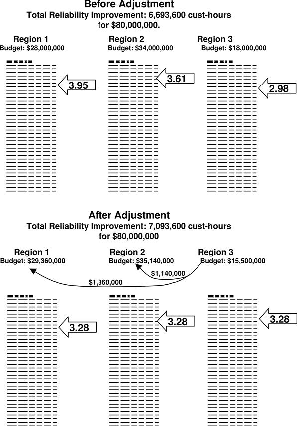
Figure 12.7 Three regions in a utility each autonomously manage their own maintenance budget using basically the same RCM procedure, locally administered by each regional office. Executive management achieves overall optimization by controlling budget allocation using the method shown in Figure 12.8, by using the individual regional projects lists (top) to determine a uniform company-wide approval score (bottom) which it applies to all three regions.
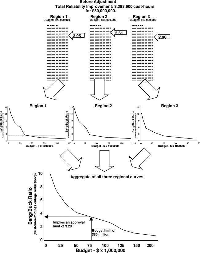
Figure 12.8 Executive management can easily control the overall maintenance budget to see both that maintenance budget is not exceeded and that RCM is optimized over the entire utility, not just within regions, with the procedure shown above. Regions submit their complete project alternatives list (top), each of which is converted to the figure-of-merit versus budget limit plot (similar to Figure 12.4) for each, and the curves summed (alternatively the lists can be added together, sorted, and plotted).
12.7 EXTENDING RELIABILITY-CENTERED PRIORITIZATION TO OTHER OPERATIONS PROJECTS
This section will briefly look at how the RCM concept can be extended to include activities and expenses that are not, strictly speaking, equipment maintenance. It will also demonstrate several nuances with respect to setting up comparisons of operations projects that differ in time or scope from one another.
Example of a Much Longer Period of Benefit than Normal Maintenance: Computerized Trouble Call Analysis
Often a utility has options with respect to spending on reliability improvement that are not classified strictly as maintenance. For example, it can implement a computerized Trouble Call Management (TMS) system to facilitate the acceptance, processing, analysis of trouble reports from its customers, and optimize the dispatching of resources and equipment for restoration and repair. Such systems do little to reduce the occurrence of equipment outages and the interruptions they cause (i.e. SAIFI). However, in the authors’ experience such systems directly reduce the duration of customer interruptions by about 15 minutes per year, and accommodate other changes (e.g., they permit more complicated and dynamic switching programs to be implemented for restoration) that make a further 5 minutes improvement. Computerized TMS systems are expensive – the advanced systems that are truly effective can cost a large utility as much as $16 million including hardware, software, training, system maintenance, and labor for operation. However, they provide long term benefits. If updated, maintained and used well, they do not lose their effectiveness at reducing reliability problems within only a few years, as do the preventive maintenance activities discussed earlier.
As an example, suppose Metropolitan Light and Power is considering a system improvement plan that is expected to provide an average 20 minutes reduction in outage time annually. Implementation will take 18 months, at a total cost of $11,300,000 for hardware, software, facilities, auxiliary equipment, labor, and training, which will be treated here as $627,778 per month average cost over the 18 month period. During that time the system provides no improvement in reliability. Subsequently, the system has a fixed operating cost of $1,700,000 per year (facilities rent and utilities, etc.), as well as a variable cost that will average an estimated $1.38/customer/year.11, 12
Table 12.12 Analysis of Long-Term Expenses and Reliability Reduction for a Trouble Call Management System
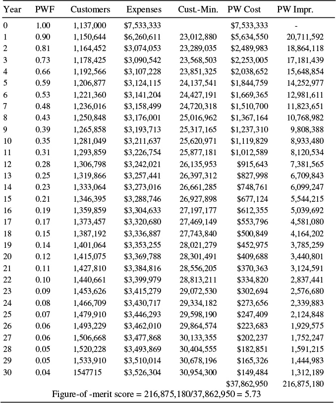
Table 12.12 lists these costs over a 31 year period, beginning with 12 months in year zero during which the project implementation begins. In year 1 the system is implemented at half year (thus there are half the variable costs and half the expected results in that year. There are no fixed costs in year 0. Customer count is expected to grow as shown (thus variable cost grow each year, too). Both future costs and future benefits are discounted using a present worth factor. As shown, the computed figure of merit is 5.73, enough to justify this TMS system against expenses in Table 12.8 or the example in Figures 12.6 and 12.7.
Figure 12.9 shows the “figure of merit so far” over time for the TMS system. When evaluating a long-term project with significant up-front expenses, it is sometimes useful to look at how good it looks in the short run, not just the long term. Since there are no improvements in year 0, and only one-half a year’s improvements in year 1, the TMS system looks rather poor on a very short-term basis. Note however that Figure 12.9 shows that its figure of merit passes 3.28 (the acceptance limit in Figure 12.8) in only 4 years. Therefore, this looks good enough to gain approval within the example evaluations used in Figure 12.8, anytime it is evaluated over a four-year or longer period.
Example of evaluating very short-term impacts and comparing options for different impact periods: tree-trimming
Tree trimming is clearly a form of “maintenance” and yet not equipment maintenance in the strictest sense. At many utilities it is administered by a separate department or from a separate budget than equipment maintenance. Since it has an identifiable cost and a direct impact on reliability there is no reason it cannot be included in RCM evaluation, with evaluation used to determine if, how much, and where tree-trimming should be used and how much budget should be allocated to it versus other maintenance issues.13 Tree trimming generally makes only a relatively short-term improvement in distribution reliability. Some utilities manage vegetation control on a three-year cycle, but two years is considered the most effective by some experts.14 Regardless, it often has a very good “bang for the buck.”
Table 12.13 shows the evaluation of six vegetation-trimming alternatives for the eastern operating district of Region 2 of the utility example used in Figures 12.6 and 12.7. The six alternatives involve two sets of three options, the sets being for programs that will provide respectively two- or three-years of benefit. Within each of these sets, there are three alternatives. These include: 1) trimming back vegetation from all primary and secondary overhead lines; 2) restricting trimming to just primary circuits; or 3) further restricting it to just along primary trunks and major branches (i.e., not along laterals).
11 This analysis assumes that none of these costs are to be capitalized. If that were the case, adjustments to the cost basis for this project might have to be done following the guidelines shown in Chapter 15 with respect to comparing capital to operating expenses.
12 There is no doubt that future improvement in hardware and software design will lower cost and improve the performance of such systems. However, the analysis is done over the long run using the costs and performance of the original system. This is what the utility is committing to, today. Future changes will justify themselves on their own merits.
13 Very often tree-trimming has a very high effectiveness per dollar and moves to near the top of the RCM list.
14 See, for example, O. C. Seevers, Management of Transmission and Distribution Systems, Fairmont Press, Liburn GA, 1995, p. 170.

Figure 12.9 Figure of merit for the computerized trouble call system as a function of the time period over which the analysis of benefits and cost is carried out. The system exceeds the 3.28 acceptance limit in Figure 12.8’s example in year four, meaning that if that utility is “looking ahead” even just four years, the TMS system’s benefit justifies taking money from the three regional maintenance budgets to pay for the system.
As mentioned above, any of these three programs can be carried out with a three-year, or two-year duration program. Two- and three-year programs vary in how far back the trimming is done, and how much off-right-of-way and off-easement trimming is attempted (with customer permission). They differ in cost (the more comprehensive trimming in the three-year program costs more) in a very subtle way, in their impact on public relations.15 Table 12.13 compares these six alternatives in absolute terms (i.e., it is not set up as a set of marginal decisions). On its own merits, any of the six programs exceeds the acceptance limit in Figure 12.8. All look like “good projects.”
15 The customer impacts differ in a way that makes it difficult to identify one program as better in this regard than the other, but on the other hand the difference is significant and should be considered. The three-year program garners a higher number of complaints about aggressive trimming, but it also involves a good deal more proactive customer contact (requests to trim trees on private property which might fall during storms) and prior notification of trimming that, while legal, might concern homeowners. Surveys indicate this leads to a mostly positive public perception of the utility’s efforts. (Table 12.13 is based on the experience of a utility in the southeast United States that decided on a three year program due to both its superior economics and because of a simple policy with regard to public relations: “all customer contact, if well-managed, is positive”).
Table 12.13 Tree-Trimming Projects Evaluated for Comparison to RCM
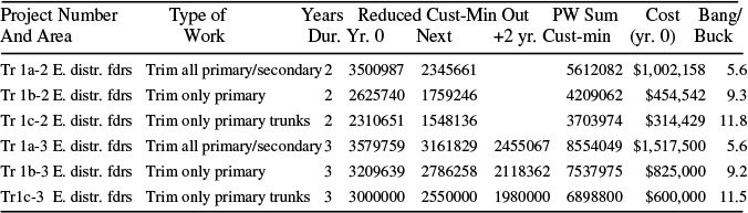
Table 12.14 Tree-Trimming Projects Ranked As Marginal Decision Chain

Table 12.15 Tree-Trimming Projects Ranked As Marginal Decision Chain with “Dumb” Alternatives Deleted

Table 12.14 shows these programs ranked in order of increasing cost, with the impacts and benefits computed as marginal values. It is now a serial list of marginal decisions for use in RCM optimization, as described in Section 12.3. The arrows at the right of the table show the serial decision chain, moving from one item to the next in the list, in this case as a series of single jumps down the list. Note that the second and fifth alternatives in Table 12.14 make little practical sense. The second on the list (Trlb-2) has a lower marginal figure of merit (3.6) than the step after it (18.5), indicating that perhaps it should be deleted from the serial list and the decision chain aimed to go around it to the next decision on the list. That would mean that the only decision to make is whether or not to take both it and the decision after it at the same time.
Similarly, item five on the list (Tr1a-2) has a negative marginal figure of merit and should not be selected. Although alternative Tr1a-2 looks good in absolute terms (Table 12.15 shows a figure of merit of 5.6), spending an additional $177,178 on it rather than the next less costly alternative (Tr1b-3) makes no sense because the additional money buys a reduction in improvement.
Table 12.15 shows the marginal decision table adjusted with items 2 and 5 in the original list deleted, and the marginal costs for items 3 and 6 changed to reflect the benefits and costs of a double jump in the table (the arrows indicate the decision sequence). There are now four items in the serial list with strictly decreasing marginal benefit/cost ratios as one moves down the list.
The optimal decision seems to be the second alternative on the list, Tr1c-3 – trimming only primary trunks, but for a three-year benefit period. This option has an absolute figure of merit of 12.5 (Table 12.13) and a marginal figure of 12.2 in this table. The next alternative in Table 12.15 has a marginal ratio of 2.8, below the utility’s service territory-wide acceptance limit of 3.38.
Results can be Valid even if Alternatives Cover Different Time Periods
The two foregoing examples bring up an important point. The evaluation method presented here is consistent with respect to different impact periods. For example, one aspect of the difference between the two- and three-year tree-trimming programs that was not addressed above was that in actual implementation, the two-year programs would be applied every two years, and the three-year programs every three years. That does not need to be considered. In the evaluation method both cost and value are discounted over time, so the computed benefit/cost ratios are consistent to shifts in time. If one takes a two-year program and shifts it two years into the future (two years after doing it the first time we will repeat it), its figure of merit be the same. Similarly, shifting a three-year program three years ahead does not change its figure of merit.
As a result, it is not necessary to compare alternative programs of different equipment programs on the basis of the same time period. Readers interested in confirming this can use the data in Table 12.13–12.15 to build tables representing a six-year period (three two-year periods versus two three-year periods) or a thirty year program (fifteen of the former, ten of the latter). The figures of merit remain the same.
12.8 OPTIMIZATION
Using Prioritization for KPIs Other Than Reliability
The prioritization method described in Sections 12.3 – 12.6 can be applied to boost the performance of any numerically representable measure, not just reliability. If the projects in Tables such as 12.8 were evaluated for extension of expected service lifetime instead of reliability, and then evaluated and ranked by what was otherwise the very same method, the resulting prioritized list would give the maximum lifetime extension possible as a function of spending. Similarly, any other numerical measure could be “optimized” by this method.
Optimization and its verb, adverb, and adjective forms are among of the most misused and abused technical terms in the power industry (and a lot of other industries). Strictly speaking, the word involves finding from among many options that which minimizes or maximizes the particular performance index. Also implicit in its application is an important concept: that there is a range or large set of possible solutions. Thus, there is no optimum answer to “What is two plus two?” There is a unique solution – just one. By contrast there are dozens of ways a utility could allocate $14 million to service, maintenance, and refurbishment of its medium voltage breakers. Every one of those ways is equivalent in terms of its basic qualitative characteristics: it spends $14 million and it spends it all on breakers. But among them, one plan might be better than another. That is the optimum plan. Thus, “optimization” involves selecting the best from among a range or set of options or alternative possibilities.
In addition, it is necessary to have a formal performance index – a definition of exactly what one considers best. Among the options might be one plan that minimizes the expected number of misoperations, essentially maximizing the reliability of the breakers themselves as a set. Another might maximize customer service reliability, something similar but subtly different. Yet another might maximizes the expected service lifetime of the equipment. Several important practical points emerge from this fact:
- One has to know exactly what one wants and be able to define it with regard to the problem. Minimize the number of breaker misoperations. Minimize SAIDI. Maximize expected number of years of service left in the equipment. Best has to have a specific definition.
- Changing the definition of best will change which option is defined as best. The three plans discussed above – minimize misoperations, minimize SAIDI, and maximize service lifetime – are each optimum as regards their particular goal.
- Optimization implies trade-offs. The optimum SAIDI plan will minimize SAIDI, but it might lead to less extension of lifetime than a plan that optimized that (and vice versa).
Prioritization methods as discussed earlier determine the best spending order for maintenance activities with regard to reliability, in a certain sense, and to a certain extent. To that extent, they optimize results. However, they are generally not considered optimization methods because:
Constraints. The real world imposes limitations on and requirements for the plans a utility can make: there are only so many breaker crews, only so much equipment can be withdrawn for service at one time, etc. These are constraints that limit the possible plans for creating requirements they must meet. In addition, practical issues of precedence, dependency and interaction create constraints in a mathematical sense (defining qualities the solution must have or cannot have). Project A has to be done before Project B can be done. Projects C and D are mutually exclusive: you can do one or the other but not both. Doing Project G reduces the expected benefit of H by 23%.
In many practical situations for both O&M and capital budget optimization, there will be more constraints involved than options to consider.16
Multi-attributes. Most organizations and executives care about more than one important attribute. Ideally, they hope to minimize SAIDI and the number of misoperations and expected equipment lifetimes. Executives realize that there are trade-offs, but everyone hopes to find ABE solutions (Almost Best Everywhere) – a plan that, while not strictly optimum anywhere, is nearly optimum everywhere (Table 12.16. The ABE solution is not optimum in any respect, but provides KPI measures within 4% in all measures, whereas any optimum solution falls up to 20% off from the optimum results in categories that are not optimized.
Table 12.16 Example of an ABE Solution

Risk and Sensitivity. The executives running nearly any business want to know the sensitivity of a particular plan to factors not entirely known or under their control (how does weather and the variable likelihood of storms play in to the possible annual SAIDI result that would be obtained?)
16 A medium size utility the authors worked with in the late 1990s used optimization to determine the best service, maintenance, and replacement program for its distribution and substation equipment. Mathematically, this resulted in 934 candidate distribution and substation programs and projects to chose from, and over 1,200 constraints of various types. The optimum plan funded 180 of the projects (about 20%) but accommodated all the constraints.
Prioritization, at least as described in Sections 12.3 – 12.6, cannot handle constraints and multi-attributes well. It cannot work against more than one attribute at a time, and it cannot directly address risk and sensitivity issues. Work-arounds to these limitations exist and are at times partly successful. Procedures that apply prioritization serially and in step-wise fashion can work around small numbers of constraints. A number of organizations have built heuristic procedures that combine multiple attributes into a single aggregated score, to give the appearance of addressing multiple attributes, and to a small extent these help. Risk and sensitivity can be studied using prioritization by slightly changing the input and looking at the results, thus obtaining sensitivities and gradually plotting risk. But in general, the basic prioritization approach – rank all candidates on the basis of merit and then select from the top of the list—cannot optimize in the sense defined above.
To find the best solution to a practical problem in the presence of constraints, when there are multiple attributes, and when risk is involved, one needs true optimization algorithms, which employ a formal numerical or logical search method to identify the optimum answer, or in some cases to find a sub-optimum answer. “Sub-optimum” sounds as if it could be far from preferable and in strict terms of the words, it means any solution less than the best. However, common mathematical parlance uses it to mean the following: “Mathematically one cannot prove this algorithm always finds the optimum solution – but what we are calling the sub-optimum solution is both a really good solution that fully meets all constraints, and the best solution that can be found.”
12.9 CONCLUSION AND RECOMMENDATIONS
It is difficult to argue against RCM, particularly in the case of a utility with significant aging power delivery infrastructure to manage. Depending on how one looks at it, RCM either maximizes the value a utility can obtain from a limited budget or minimizes the cost to obtain any targeted level of reliability improvement through maintenance.
Utilities with aging power infrastructures have need of more than the average amount of results from inspection, testing, preventive maintenance, and repair. Often they have fewer budget dollars than required for traditional maintenance approaches. As a result they need all the advantages possible with respect to getting the most “bang from the buck” from maintenance. RCM does precisely this. It is implementable with information that any distribution system owner (industrial or commercial or public utility) has, and uses only straightforward procedures (electronic spreadsheets, good record-keeping), although those procedures do have to handle large amounts of projects and alternatives to be effective. Therefore, it is strongly recommended.
Table 12.17 lists a number of recommendations for maintenance prioritization that generally hold true to all utilities but particularly those with aging infrastructures to manage. The rest of this conclusion discusses each item in the table in more detail.
Apply Prioritization to All Parts of the System, Not Just One Level or One Department’s Venue
RCM can work at all levels and for all types of equipment at a utility. There is no reason to limit its scope to only one type of equipment (e.g., power transformers) or to within only one department (Substation Operations). In fact, as will be covered in Chapter 14–15, the basic concept should be extended to all activities, and all spending throughout the utility, not just restricted to maintenance.
Zero-Base All Decisions
All good O&M planning begins with an assumption that nothing is sacred. Any action has to justify itself on the basis of the benefits it makes compared to the costs it requires. All possible O&M actions are in competition with one another for funding. The most effective will win.
Apply Prioritization Using Intra-Project Alternatives’ Evaluation
The improvement in “bang for the buck” wrought by applying the optimization to determine both what equipment should be maintained, and how maintenance on each unit should be done can be substantial. The added value is well worth the cost of the more comprehensive and detailed analysis required.
Table 12.17 Guidelines for Maintenance Scheduling on Aging Infrastructure Systems
|
• Apply the RCM concept using intra-project alternatives’ evaluation in the optimization • Use a reliability definition as close as possible to regulatory mandate or formula • Zero-base all decisions • Apply intra-project alternatives evaluation for RCM • Use the same reliability definition in all regions and for all departments • Use generic categories of work and equipment along with pre-defined expectations and costs • Do not confuse inspection period with improvement period • Rely on inspection and testing to carry a lot of the burden in any maintenance program |
Minimize the Same Reliability Definition Everywhere
Similarly, unless regulatory mandates decree different definitions of reliability or “good customer service” be applied in different areas of the system, the same definition should be used in all RCM in all regions and all departments.
Use a Reliability Definition as Close as Possible to Regulatory Mandate
As discussed in Section 12.3, while conceptually there may be indices (definitions of reliability measure) that make sense or seem fair from one perspective or another, ultimately a utility should let the regulatory process define “what is wanted.” Once defined, this should be the performance index used in all decisions aimed at “improving reliability.”
Use Generic Categories of Work and Equipment Along with Pre-Defined Expectations and Costs
As discussed in Section 12.3, use of categories for both equipment condition and service classes both simplifies application of RCM on a large scale, and keeps it within in a context of using cost and results factors in only a legitimate probabilistic, manner. Categorization within a rigorous format also discourages adjustment of data by individuals based on claimed “judgment” or special knowledge (i.e., fudging the data).
Do Not Confuse Inspection Period with Improvement Period
The periodicity needed for inspection and the period during which improvements from service are expected to last are not the same. Section 12.3 (Figure 12.6) recommended that the period of improvement due to servicing a unit be modeled as relatively short-term. However, short as it may be, it is often longer than prudent periods for inspection. For example, “major service” might produce an improvement in expected reliability of a transformer that lasts five years. But the utility might decide it is prudent to inspect the unit annually, because problems with something other than what was serviced last time could develop.
Expect Inspection and Testing to Carry a Lot of the Burden
In any optimized program, inspection, testing, and diagnostics carry a good deal of the weight of improvement. In a very real sense, a good RCM plan is its own type of “just in time” system: frequent inspections and testing tend to uncover problems before they occur; a system based on these problems where repairs are only made to items that need to be replaced; and periodic scheduled repair/replacement. On the other hand, something may be replaced that doesn’t seem to really need it, just because it’s time.
REFERENCES AND BIBLIOGRAPHY
R. E. Brown, Business Essentials for Utility Engineers, CRC Press, Boca Raton, 2010.
J. J. Burke, Power Distribution Engineering – Fundamentals and Applications, Marcel Dekker, New York, 1994.
P. Gill, Electrical Power Equipment Maintenance and Testing, Marcel Dekker, New York, 1998.
Institute of Electrical and Electronics Engineers, Recommended Practice for Design of Reliable Industrial and Commercial Power Systems, The Institute of Electrical and Electronics Engineers, Inc., New York, 1990.
H. H. Malik, A. A. AlArainy, and M. I. Qureshi, Electrical Insulation in Power Systems, Marcel Dekker, 1998.
O. C. Seevers, Management of Transmission and Distribution Systems, Fairmont Press, Lilburn 1995.
W. A. Thue, Electrical Power Cable Engineering, Marcel Dekker, New York, 1999.