
7 Aging Equipment and Its Impacts
7.1 INTRODUCTION
Aging equipment is undoubtedly the primary cause and effect associated in most people’s minds with the term “Aging Infrastructure.” And while there are other significant factors involved as were summarized in Chapter 1, there is no doubt that aging infrastructures present an incredible challenge largely due to the effects of aging equipment. Aging equipment has high failure rates and requires, proportionally, more inspection and maintenance cost. Often parts and service equipment are hard to come by (and expensive).
This chapter looks at equipment aging – what it is, how it impacts the various types of equipment, and how those changes affect the reliability and economy of a power system’s operation. Invariably failure rates increase with age, usually in an exponential manner. But characteristics vary depending on equipment type (aging impacts poles very much differently than say, cable) and conditions of use. Most important to the modern distribution utility is how an aging base of equipment changes the performance (reliability and economy of operation) of the system as a whole, and impacts the quality of customer service.
This chapter begins in Section 7.2 with a qualitative look at aging and its impacts on equipment, discussing the different categories of aging impact, and the general characteristics of aging on equipment such as transformers, poles, cables, etc. Section 7.3 then looks at quantitative trends in failure rates as equipment gets older – how and why do failure rates increase? This section raises an interesting concept – what would exact information on when a particular unit of equipment will fail be worth, and how could a distribution utility utilize that information? Section 7.4 delves into the impact that aging and failure rates have on the installed base of equipment in a utility system and the repercussions on cost and service quality that result. Section 7.5 concludes with a summary of key points.
7.2 EQUIPMENT AGING
All electrical equipment kept in service ages. During every year of service the equipment becomes a year older. One consequence of this aging is gradual deterioration of the physical and electrical strengths of the equipment, until at some point failure occurs one way or another – the end of the equipment’s useful lifetime. Table 7.1 shows several types of deterioration that affect older equipment. The “caused by” columns show which of the three primary types of aging, covered in Table 7.2, lead to the respective type of deterioration.
Table 7.1 Types of Deterioration Causing By Aging
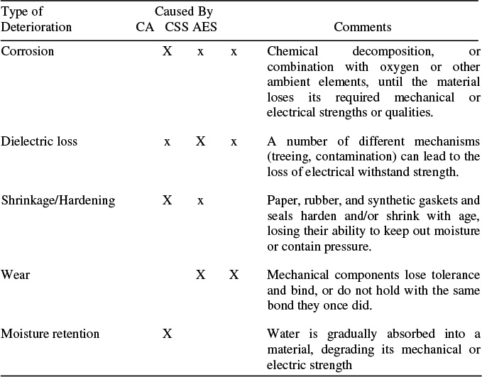
Table 7.2 Categories of Equipment Aging Impact and Their Meaning
Types of Aging Impact
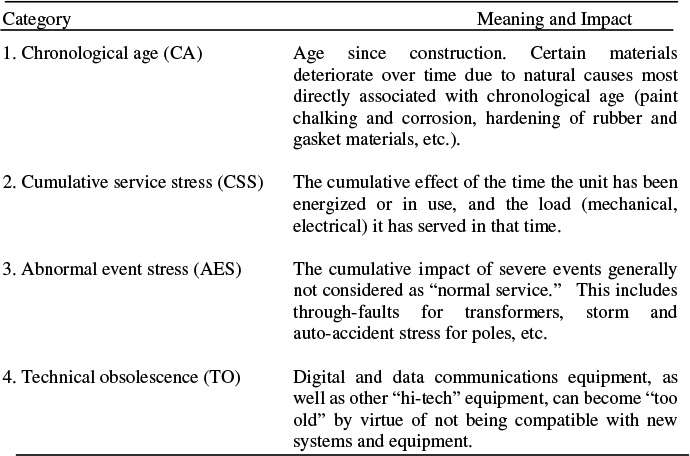
Aging can having any of several particular meanings with respect to power system equipment, as shown in Table 7.2, which lists four specific categories of aging and their impacts. Generally, the terms “aged or old” and “aging” are used to refer to some non-specific combination of all four effects, with the understanding that the equipment is not as useful or dependable as similar equipment of lesser age.
Chronological age
Certain materials such as paint, paper and fabrics, rubber and synthetic gaskets and seals, and insulation, deteriorate over time. Time since manufacture alone is the direct cause of this type of deterioration. Thus, seals and gaskets begin to harden, and paint to chalk, as soon as a transformer or breaker is built, progressing at much the same rate regardless of whether the unit is installed and in service or kept in inventory in an equipment yard. A creosote pole will dry out and begin the very slow process of chemical breakdown of its preservative whether or not it is stored in an equipment yard or put in the ground. It will however, begin to rot at the ground line only after being put in the ground, particularly if the soil around it is moist and of the right pH.
As the pole example in the last sentence illustrates, very often the rate of deterioration over time is exacerbated or mitigated by ambient conditions. Transformers, poles and cables stored outside and subjected to summer heat, winter cold, direct sunlight and ambient moisture, will deteriorate faster than if kept in sealed, temperature-controlled and dehumidified warehouses. Deterioration due to chronological aging can be cut by two thirds in some cases if the equipment is keep in a controlled environment. Generally, “chronological aging” rates and average lifetimes assume that the equipment is installed in typical ambient service conditions (i.e., poles and transformers are kept outside whether in service or not).
In many cases, the deterioration that would occur due to time alone is accelerated by the stresses caused by putting the equipment in service. Hardening of gaskets and seals, and paper insulation, will occur at a faster rate when a transformer is operating (heat generated by electrical losses will accelerate the deterioration processes).
In some cases, however (i.e., paint chalking and some types of corrosion), the rate of deterioration does not depend on whether the unit is in service. And in a few situations, putting a unit in service will reduce the rate of chronological deterioration. For example, energizing a power transformer being kept for standby service creates a low level of heating (due to no-load losses) that “cooks” any moisture build-up out of the unit, slowing that rate noticeably.
Cumulative service stress
Certain types of deterioration occur only, or primarily, due to the use or operation of the unit for its designed purpose, and are proportional to the time or the cumulative level of use in service, not chronological time. There are three primary types of processes involved:
1. Electromagnetic field stress established when a cable or unit of equipment is placed in service can lead to degradation of dielectric strength and in some cases, promote corrosion. Essentially, applying voltage to the device produces a stress that will eventually break down insulation and accelerate some chemical processes (particularly if the unit is not grounded well or cathodically protected). This type of stress depends only on the voltage. It does not depend on the amount of current (power) the unit is handling.
Every unit of electrical equipment – transformer, cable, bell insulator – is always designed to withstand a nominal voltage, that which it can withstand safely and dependably over a long period of time (decades). But, given enough time, the electromagnetic stress from that voltage will lead to various types of insulation breakdown, which can include treeing, attraction of impurities that build flashover paths, etc. Eventually, over a century (post insulators), or only a period of several decades (UG cable), the insulation will fail for this reason alone.
In most cases the deterioration rate due to this cause is very voltage sensitive. Raising voltage even slightly will increase stress a good deal. Thus, higher voltages, due to operating the unit at the high end of its nominal range, or to misoperation, switching surges, or lightning, can accelerate this deterioration, sometimes quite dramatically. Similarly, lowering the voltage on equipment that is suspected of being weak (old cables) to the low end of the permissible scale (e.g., .95 PU) can often reduce stress, deterioration and failure rates significantly. And of course, voltage that reaches too high a level – above the tolerable range – leads to immediate failure.
2. Wear. Parts that move against one another, in devices such as tap changers, capacitor switches, circuit breakers, load break switches, etc., wear. The movement gradually erodes material in the moving junction between parts, loosening tolerances and often scouring smooth bearing surfaces. Such wear can lead to binding of moving parts and failure to operate, or to operate slower than necessary (breakers).
The term “wear” can also be applied to a type of mechanical deterioration that occurs in parts that are not technically moving against one another. An example is in overhead conductors and their splices, terminations, and support brackets. The conductor “moves” in the sense that it sways in the wind, and expands and shrinks, and sags more or less, with temperature (and loading). Over decades, this movement can lead to loosening of the bond between clamps and conductor, or within splices or termination fittings, and even to cracking of the conductor material itself. Eventually something breaks and the line falls.
This gradual deterioration is accelerated greatly by aeolian vibration. Wind blowing across the conductor sets in motion a resonant vibration, much like blowing on a harp string might cause it to hum. This vibration stresses the bonds in splices, brackets and clamps, and can fatigue the metal strands of the conductor, over a period of only months in extreme cases. Various types of vibration dampers are available to fit to conductors to stop such vibration, but these are usually fitted only to known or suspected cases of heavy vibration. Most overhead spans experience a slight amount of this vibration, and over decades it leads to a degradation of mechanical strength in the conductor and its fittings.
3. Heat stress. Higher temperatures accelerate many of the physical and chemical mechanisms involved in material’s deterioration, to the point that heat can be considered electrical equipment’s worst enemy. In electrical equipment like transformers, regulators, and motors, heat is generated by electrical losses in the equipment. The higher temperatures created as a result cause deterioration of materials in insulation, gaskets, seals, the transformer oil itself, and in some cases, the metal in conductors and/or mechanical components. Similarly heat affects all electric equipment, “aging” or ruining the functionality of various materials or their components. Parts that should be soft and expanded, so they seal well, shrink. Parts that should insulate lose dielectric strength. Metal expands, binding and wearing, or, at very high temperatures anneals so that it becomes brittle and of low strength – essentially a different type of alloy.
In almost all cases, the rate of deterioration of a component or material is a function of the temperature, generally increasing exponentially with a temperature up to some maximum-tolerable temperature beyond which the material fails immediately. The relationship is exponential – a device might be able to operate for decades at 80°C, for several years at 90°C, for a week at 100°C, and for only a few hours at 110°C.
In addition, temperatures that reach certain levels can cause internal physical changes in some types of electrical equipment, changes that promote misoperation. For example, in a power transformer, extreme heating of the windings (due to losses from very high loadings) can cause hot spots on the core that are hot enough to create gassing or boiling of the oil. The gas introduced into the oil by the bubbling contaminates the oil’s ability to act as an insulating medium, and a “bubble path” can provide a route for flashover, leading to immediate and catastrophic failure.
In mechanical devices such as breakers, load tap changers, and motors, high temperatures can cause swelling of mechanical parts, leading to binding (bearing tolerances are reduced to the point that the device will not operate) and misoperation, and/or high rates of wear. In overhead conductor, high enough temperatures (typically caused when losses generate heat sufficient to create a 100°C rise above ambient) will anneal the conductor material. As a result it hardens, becomes brittle and loses its elasticity and mechanical strength. Vibration from wind and the natural expansion of heating and cooling from diurnal temperature variations then quickly leads to minute cracking and mechanical failure and the conductor breaks and falls to the ground.
The deterioration caused by high temperature is cumulative – i.e., a period of high temperature will cause deterioration that will not be “undone” when temperatures fall. A device will suffer gradual deterioration of its components, equal to the cumulative stress of high temperature over its service life to date. Since heat (the cause of high temperatures) is due to load (the load current causes losses that create the heat), power engineers often associate deterioration rate directly with load: higher levels of load lead directly to higher rates of deterioration. The term “loss of life” refers to the rate of equipment lifetime loss associated with a particular loading (heat and temperature) level for the equipment.
Many of the chronological aging processes discussed earlier are accelerated if the device sustains high temperatures for long periods of time (as is common for many electrical devices). Thus, chronological aging and cumulative service stress is not, in practice, completely independent.
Abnormal event stress
Over its service life, any particular unit of power system equipment is likely to see a number of “events” which lie outside the normal conditions expected in service. These include electrical events such as through-faults, switching surges, and lightning strikes, and/or harsh mechanical events such as automobiles striking the device (i.e., a pole or pad mounted device), high ice loadings from freak winter storms that mechanically stress overhead conductors, and similar situations.
Auto accidents and storm damage are prime causes of wood pole and metal structure failure, and somewhat unavoidable given that these structures are often placed on public easements and parallel roadways. However, most of these events are reported (many result in immediate failure of the pole, or equipment at the top of it) so the utility is at least aware of the event and can inspect and repair any damage done.
Ice loadings are another stressful mechanical factor, but one that is more difficult to track. During severe winter weather, ice will accumulate on overhead conductors. Given extreme conditions, several inches of ice can accumulate, weighing many hundreds of pounds per span. The cumulative weight of conductor and ice can exceeds the strength of the line, and it will part, falling to the ground. However, in the vast majority of winter storms, icing does not lead to failure – the weight is tolerated without any damage or deterioration.1 When the ice melts after the storm, the conductor is, if not “good as new,” as good as it was before the storm.
1 Conductors, particularly those with steel reinforcement (ACSR – Aluminum Clad Steel Reinforced Conductor) are designed to have high mechanical strength to deal with periodic severe ice loadings. In some areas of the world (e.g., parts of Saskatchewan) the distribution utility uses an entirely steel wire in its OH distribution sacrificing the lower resistance of aluminum for the superior ice loading capability of pure steel wire.
But in between these two situations – outright failure on one hand and no damage done on the other – is a narrow range of “damage-done” cases that are particularly vexing to utilities. The ice loading on a particular span of an overhead conductor might reach a level that does not cause immediate failure, but is sufficient to stretch the conductor to its elastic limits, or over-stress clamps, splices, etc. This leads to accelerated deterioration and failure soon afterward. The utility has no way of knowing if any portion of its overhead lines were so affected and if so, which portions.
Through-faults are the most stressful event routinely seen by many transformers, from the standpoint of gradual deterioration leading to failure. A device downstream of the transformer experiences a fault, and for a brief time until a circuit breaker clears the fault, the transformer sees current flow through it that is from three to fifty times normal maximum. Heating caused by this high current is usually not the major impacting process – in most cases the fault current lasts but a few cycles and little heat energy is generated.
Instead, the most common damaging effect of through-faults is the magnetic field created by the very high current levels, and its shock impact on internal components. Transformers (and motors and voltage regulators as well) are designed so that the current flow through them causes an intense magnetic field – required for their operation. But a through-fault multiplies that field strength in direct proportion to its greater current level, creating a tremendous magnetic field and compressing or pulling apart nearby components, etc.
The magnetic force from a severe fault can create tremendous force. If high enough, this force can literally rip connections loose inside the transformer, leading to immediate and perhaps catastrophic failure. But typically, in a well-planned power system, fault currents are limited by design and operation to levels not so severe that they lead to such problems. Still, the mechanical impulse from a “tolerable” through-fault will make a large power transformer, weighing many tons, shake and “ring” as if it had been dropped several feet, and has an overall effect on it similar to such abuse. The cumulative impact of a number of such severe shocks over a transformer’s lifetime can be a significant loosening of the core stack, and stretching and twisting of windings and connections – a general weakening of the mechanical integrity of the unit.
The cumulative impact of through-faults is thought by many power equipment experts to be the leading cause of power transformer failure. There are recorded cases where transformers (and motors, and voltage regulators) fail when a through-fault occurs, generally when such faults occur during peak loading conditions (when the transformer is already quite hot from high loadings and thus under a good deal of stress). Previous events have weakened the overall integrity of the unit until this one last through-fault is sufficient to cause failure.
However, more often than not, failure does not occur during or immediately after a through-fault. Since peak loads occur less than 5% of the time most through-faults happen during off peak times when conditions in the transformer are at low stress levels. Often the unit tolerates the fault at that time, but the damage has been done. The unit subsequently fails at a later time – hours, days, or even weeks afterward – when it is first exposed to prolonged peak load stresses.
Few utilities have dependable, easy to access records on the through-faults experienced by major transformers during their lifetimes. As a result, one of the most useful records of cumulative stress needed to determine present condition is unavailable to engineers and planners trying to deal with aging equipment and the estimation of its remaining lifetime.
Lightning strikes are severe-stress events that often lead to immediate failure of a device, almost a certainty in cases where the device is struck directly. Lightning is a pure current source, with the current flow being from ten to one hundred times the normal fault levels seen in power systems. A lightning strike can cause an immense “through-fault” like failure, or lead to a voltage flashover that causes other problems.
Failure modes due to lightning strikes are complex, and not completely understood, but failure occurs mainly due to heat. Although very brief, the incredible magnitude of the lightning current, often over 500,000 amps, creates heat – trees hit by lightning explode because the water in them is instantly vaporized. Similar impacts occur in electrical devices. In other cases the magnetic shock of high current does the damage.
There is considerable evidence that a good deal of damage can be done to electric equipment by indirect lightning strikes. A lightning strike to the ground near a substation can cause high voltages and or erosion of grounds. A strike in the ground may also travel to a nearby UG cable or grounding rod, burning it badly.
Lightning strikes to overhead lines often cause immediate failure, but can instead cause a flashover, which, due to breaker operation and an interruption, leaves no outaged equipment. However, the equipment may be damaged to the extent that it will fail in the next few weeks or months. In some utility systems, there is a statistically significant increase in service transformer and line failures after the annual “lightning season.”
Abnormal stress events can occur from time to time in the life of any electrical equipment. In some cases, the severity of one event leads to immediate failure, but often it is the cumulative impact of numerous events, over years or decades, that gradually weakens the device. Sometimes these events cause deterioration similar to that caused by time or service, but most often the degradation in capability is different – through-faults loosen transformer cores and twist internal fittings in a way that no amount of normal service does.
Technical obsolescence
Most types of equipment used in power systems are from “mature” technologies. Although progress continues to be made in the design of transformers, breakers, and so forth, these devices have existed as commercial equipment for over a century, and the rate of improvement in their design and performance is incremental, not revolutionary. As a result, such equipment can be installed in a utility system and be expected to “do its job” over its physical lifetime – obsolescence by newer equipment is not a significant issue.
A forty-year old transformer in good condition may not be quite as efficient, or have as low maintenance costs as the best new unit, but the incremental difference is small and not nearly enough to justify replacement with a newer unit. However, in most cases, if a unit is left in service for a very long time, the issue of spare parts will become significant. Some utilities have some circuit breakers that have been in service 50 years or more. Replacement parts and fittings are no longer manufactured for the units, and have to be customized in machine shops or scavenged from salvaged equipment.
But a noticeable segment of the equipment used in utility power systems does suffer from technical obsolescence. The most often cited cases are digital equipment such as computerized control systems, data communications and similar “hi-tech” equipment associated with automation, and remote monitoring and control. Typically anything of this nature is eclipsed in performance within three to five years, often providing a utility with a new level of performance that it may wish to purchase. The older equipment still does its job, but is vastly outperformed by newer equipment. Economic evaluation of the benefits of the new systems can be done to determine if the improvement in performance justifies replacement. Often it does.
But beyond performance issues alone, there are other factors that mitigate against this equipment remaining in service for decades. First, since in some cases spare parts are made for this type of equipment for only a decade or so after manufacture, there is no viable prospect of leaving the equipment in place for many decades. Secondly, even if parts are available, newer equipment requires different test and maintenance procedures. Qualified personnel to make inspections and repairs become more difficult (and expensive) to find.
While digital equipment used in control and automation is the most obvious case of “technical obsolescence,” there is a much more dramatic, and significant case that is causing perhaps the most contentious issue facing the power industry as it moves toward full deregulation. The issue is a stranded assets and the cause is technical obsolescence of generating plants. Many utilities own generating units that are fifteen to twenty years old. These units are not fully depreciated – when the units were built, the utilities borrowed money to pay the expenses, financed over thirty-year periods, and they still owe significant amounts on those loans.
But the technology of generator design has improved considerably since those units were built. Newer generators can significantly outperform those older units, producing power for as much as a penny/kWh less and requiring less frequent and costly O&M and fewer operators. In a deregulated market, merchant generators can buy these units and can compete “unfairly” with the utility’s older units. Thus, these older units are “stranded” by the shift to deregulation – the utility was promised cost recovery when they were purchased, but now faces competition due to technical obsolescence, and a drop in the sales that were expected to provide revenues to pay off the loans.
In the T&D arena, technical obsolescence will continue to be an important factor in control, automation, and metering areas. In addition, a high rate of technical progress will continue to impact power system equipment areas such as distributed generation, power electronics/power quality equipment, and home and building automation and control systems.
Lack Of Proper Care Can Accelerate Aging Effects
Lack of proper maintenance or inattention in setup and/or operation can, in some cases, lead to excessive deterioration due to secondary impacts (e.g., neglected seals let in moisture which leads to dielectric failure). The degree to which neglect leads to premature failure depends on the type of device and the extent to which its design depends on periodic maintenance.
Equipment with moving mechanical components tends to be most sensitive, that sensitivity proportional to the frequency of mechanical operation. Thus, tap changers and voltage regulators are most prone to early failure due to neglect. However, upon failure they can often be repaired by performing the maintenance or replacement of parts that has been deferred.
On the other extreme, most service transformers and residential power meters are essentially no-maintenance devices – they can be installed and expected to last for a normal lifetime without any maintenance. The first attention they get subsequent to installation is when they fail to do their job for some reason. At this point they are usually replaced. Equipment requiring little or no maintenance generally has only one “service mode” replacement.
Neglect or stupidity in setup or operation is another matter entirely. A neglected aspect of equipment use, often leading to rapid deterioration is poor grounding. Equipment may not be well grounded when installed, or the quality of the ground might degrade over time due to corrosion of clamps, etc. In either case, a weak ground can cause higher than normal and/or abnormal currents during “normal operation” accelerating the deterioration caused by normal service stresses. More critical yet, poor grounds often exacerbate the impact of lightning, switching surges, and through-faults to the point that the stress caused is two to five times greater. Failure is nearly assured.
Other types of poor setup include mismatch of transformer impedance in multi-phase banks composed of single-phase units, incorrect settings for regulators, and similar inattention to details in equipment utilization.
Loss of Life and Load-Related Lifetime
Overall, of all the deterioration modes mentioned above, the major contributor to aging of electrical components in a power system is high temperature, a service-stress-related cause. High enough temperatures will cut short a device’s life instantly. More typically, the cumulative effect of high temperatures over years of service leads to deterioration of key elements inside the device until they fail, leading to cessation of function, and often ruining the device.
The heat generated by electrical loss causes high temperatures. Those losses are a function of the electric load on the device. Therefore, the major component of aging is related directly to the loading on the device. While other types of deterioration proceed in parallel, usually this is the one that leads to failure (unless a high incidence of abnormal events fails the unit first).
For this reason, power system equipment engineers often speak of load-related lifetimes and “loss of life” of a transformer, motor, regulator or other component, as a function of its loading. Figure 7.1 shows the expected lifetime of one particular transformer if loaded to various levels. The unit can be expected to last 40 years (350,000 hours) if loaded continuously to 80% of its rated load, or only
7.5 years if loaded to 100% on a continuous 24 hour a day basis (solid line). If serving a typical utility load (time-varying load with a 60% annual load factor and peak periods of four hours duration) the unit has an expected lifetime of 40 years when serving a peak load equal to 100% of its rating (dotted line).
Thus, operation at 150% of rated load (estimated lifetime, 350 hours) can be likened to accelerating the unit’s normal 40-year (in utility service) lifetime by a factor of 1,000. The unit looses 1,000 hours of expected operational service lifetime for every hour of operation at 150%, i.e.; every hour of operation at this loading level uses about 40 days normal service lifetime. Most other types of power system equipment have qualitatively similar lifetime versus loading relationships.
While this is a dramatic acceleration in loss of life, most utilities make it policy to operate a transformer at much higher loads during contingencies. Under emergency conditions, transformers are often operated at load levels up to 166% of rating. At this load level, expected lifetime is only 120 hours and every hour of operation uses the equivalent of four months of normal operation (see Chapter 8 for a discussion of contingency loading policies).
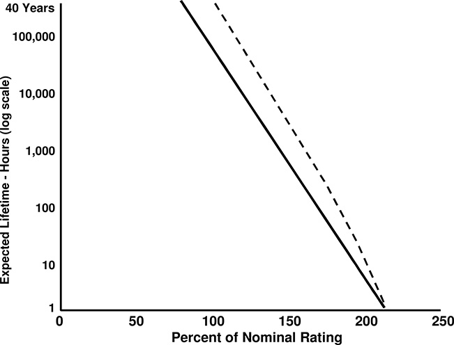
Figure 7.1 The expected lifetime (time to 50% likelihood of failure) for one particular type of power transformer, as a function of the loading in percent of nominal rating. Solid line shows lifetime for constant loadings. Dotted line shows expected lifetime if serving an annual load curve of 63% load factor with a peak load measured at 100% percent of rated capacity.
The reason is one of economics, and makes sense in almost all cases. Given that peak loads occur only occasionally, a transformer that has been installed so that it is expected to take up to 166% of its normal peak load during a contingency will probably see only 20 hours of such intense service during a 30 year plus service lifetime. Most contingencies will occur off peak when loading and thus the stress is far lower. Those 20 hours of loading will cumulatively lead to a loss of 7 years of the expected 40-year lifetime.
But the benefit gained (contingency coverage of other transformers) is considerable, because other options for that coverage are costly. And the savings lie entirely in the present – it has a present worth factor of 1.0. By contrast, the loss in life is realized at the end of the transformer’s life, 33 years into the future (40 years minus 7). Present worth factor, in that timeframe, is minute (about 3%) so the lost service life has minimal value by comparison. Simply put, benefit exceeds cost.
Of course, a utility can get into trouble, as many have, by putting old transformers under such high levels of stress during contingencies. Many utilities have transformers that have successfully made it through forty or more years of service, during which time the units were never exposed to such high contingency loadings, due to the more relaxed loading standards that existed in the traditional utility industry. The units are partly deteriorated and weaker than new – they may have only a decade of remaining expected life. But due to financial pressures, the utilities have to switch to a policy of intense contingency loading. The problem created is that the stress of this use may absorb most of what life remains.
“Old” Depends on the Expected or Design Lifetime
Finally, it is worth noting that whether equipment is old or not depends on the expected equipment lifetime, as designed. A 20-year old wood pole is not really old (expected lifetime is at least twice that), but a 20-year old substation RTU is. A 40-year old span of ACSR is not yet really old, but a forty-year-old set of capacitor switches is.
Electrical equipment can be designed to withstand any degree of deterioration, by building it from a higher grade of materials that assures longer life (slower deterioration rates, or in some cases immunity from deterioration). Similarly, heavier material (e.g., thicker paint) can be used to allow more deterioration to occur before failure occurs, or because harsher conditions are expected. This results in a longer expected period of time, service, or abnormal events before degradation leads to failure or misoperation.
But such measures cost money. Thus, ultimately equipment lifetime is somewhat a function of cost. In general, most electrical equipment like transformers, breakers, and regulators is designed to withstand the chronological, service, and abnormal events associated with about 40 years of service under typical ambient conditions and loading. Overhead conductors and its ancillary equipment generally have a lifetime of 60 years or more (the required mechanical strength pretty much assures immunity from electrical, thermal, and/or rapid deterioration unless abused by very harsh service). Wood poles have about a 40 – 75 year expected lifetime, depending on quality and soil conditions and steel structures typically last up to 100 years. Underground cable often has the shortest expected lifetime. Although paper insulated, lead-covered (PILC) cable has an expected lifetime of up to 60 years if well-cared for, most other types of cable have lifetimes between 20 and 35 years.
Table 7.3 Effects of Power System Equipment Aging, in Order of Importance
|
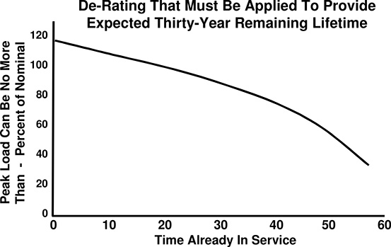
Figure 7.2 Example of the impact of “de-rating” a unit in order to increase expected lifetime. See text for details. (Note: This curve is not general; it does not accurately apply to all transformers.)
Worn out equipment usually is really worn out
Usually, all of the types of deterioration discussed above are occurring simultaneously in any electrical device or line. Corrosion, dielectric breakdown, wear, and loss of mechanical strength all proceed at their own paces. Failure of a unit like a breaker or transformer is a type of horse race between the various failure modes that could fail it. The unit will fail when the first of these various types of deterioration reaches the point where it causes misoperation or catastrophic failure (the device destroys itself).
One element of good design for power system equipment is a balance among the expected lifetimes of all these various components. This just makes sense: if a transformer’s case is known to fail within 50 years, it is a waste of money to install a core that can easily last 100 years. Good design tries to balance the various strengths and amounts of materials in a unit so that all have roughly the same lifetime in typical service. This means that when failure occurs or is imminent due to one particular type of deterioration, the unit is most likely worn out in all its other deterioration modes, too. It may not be worth repairing because such repair essentially requires rebuilding and or replacing everything.
Effects of Equipment Aging
Table 7.3 lists the effects of equipment aging, in rough order of importance to most electric utilities. As units age they have a higher likelihood of failure and misoperation (all equipment). In some cases aging results in a reduced capacity or rating (nearly all equipment, whether recognized or not – this will be discussed in the next section). Some types of devices also see increased electrical or mechanical losses with age (some motors and transformers). In other cases, the device may produce more sound pollution as it may age (motors and transformers, due to core or stator stack loosening, etc.).
By far the most significant factor, and the major concern to a distribution utility, is the top effect listed in Table 7.3: increasing likelihood of failure. The next section discusses this in great detail.
De-rating to Preserve Remaining Lifetime
Table 7.3 lists de-rating as one impact of aging. Since the major modes of deterioration and failure are often heat-related or other service-stress created causes, one option available to an equipment operator is to lower the loading (i.e., cause of stress) in order to increase the expected lifetime of the equipment.
Figure 7.2 shows a de-rating curve for a power transformer that has an expected 40-year lifetime and has already seen 30 years of service at designed load levels. At this point, it has an expected 14 years of service left if kept at its present service level where peak load is 100% of its rating.2 If the owner wishes to extend the expected time-to-failure to 40 more years of service, he must reduce loading by 29%, to only a peak of 71% of the unit’s rating. Similarly, if this unit is loaded to 110%, it will very likely fail within a few years. Thus, the owner can balance the annual value to be obtained from the unit (how much power it handles) against the number of years that value is expected to be provided by the unit.
7.3 EQUIPMENT FAILURE RATE INCREASES WITH AGE
All equipment put into service will eventually fail. All of it. Some equipment will last longer than others will and often these differences in lifetimes will appear to be of a random nature. Two apparently identical units, manufactured to the same design, from the same materials, on the same day at the same plant, installed by the same utility crew on the same day in what appear to be identical situations, can nonetheless provide very different lifetimes. One might last only 11 years, while the other will still be providing service after 40 years. Minute differences in materials and construction, along with small differences in ambient conditions, in service stress seen by the unit, and in the abnormal events experienced in service, cumulatively lead to big differences in lifetime.
In fact, generally the only time one finds a very tight grouping of lifetimes– i.e., all of the units in a batch fail at about the same time – is when there is some common manufacturing defect or materials problem – a flaw – leading to premature failure.
Predicting Time to Failure
High failure rate and uncertainty make for a costly combination
As a conceptual learning exercise, it is worth considering how valuable exact knowledge of when any particular device would fail would be to a distribution utility. Suppose that it were known with certainty that a particular device would fail at 3:13 PM on July 23. Replacement could be scheduled in a low cost, low impact on customer manner prior to that date. There would be no unscheduled outage and no unanticipated or difficult to manage costs involved: impact on both customer service quality and utility costs could be minimized.
2 It does not have only ten years of expected service left. This is a “survivor” of 30 years service. As such, statistically, it has a likelihood of lasting more than the average 40 years expected when it was new. Essentially it is making up for the few other units of its type that failed prior to 30 years of service, keeping the average at 40 years service.
It is the uncertainty in the failure times of power system equipment that creates the high costs, contributes to service quality problems, and makes management of equipment failure so challenging. The magnitude of this problem increases as the equipment ages, because the failure rates increase: there are more “unpredictable” failures occurring. The utility has a larger problem to try to manage.
Failure time prediction: an inexact science
With present technologies, it does not seem possible to predict time-to-failure exactly. In fact, capability in failure prediction for equipment is about the same as it is for human beings.
1. Time-to-failure can be predicted accurately only over a large population (set of units). Children born in 2000 in the United States have an expected lifetime of 76 years, with a standard deviation of 11 years. Service transformers put into service in 2000 have an average expected lifetime of 43 years with a standard deviation of 7 years.
2. Assessment based on time-in-service can be done, but still leads to information that is accurate only when applied to a large population. Thus, analysts can determine that people who have reached age 50 in year 2000 have an expected 31 years of life remaining. Service transformers that have survived 30 years in service have an average 16 years of service remaining.
3. Condition assessment can identify different expectations based on past or existing service conditions, but again this is only accurate for a large population. Smokers who have reached age 50 have only a remaining 22 years of expected lifetime, not 31. Service transformers that have seen 30 years service in high-lightning areas have an average of only 11 years service life remaining, not 16.
4. Tests can narrow but not eliminate the uncertainty in failure prediction of individual units. All the medical testing in the world cannot predict with certainty the time of death of an apparently healthy human being, although it can identify flaws that might indicate likelihood for failure. Similarly, testing of a power transformer will identify if it has a “fatal” flaw in it. But if a human being or a power system unit gets a “good bill of health,” it really means that there is no clue as to when the unit will fail, except that that failure does not appear to be imminent.
5. Time to failure of an individual unit is only easy to predict when failure is imminent. In cases where failure is due to “natural causes” (i.e., not due to abnormal events such as being in an auto accident or being hit by lightning), failure can be predicted only a short time prior to failure. At this point, failure is almost certain to advanced stages of detectable deterioration in some key component.
Thus, when rich Uncle Jacob was in his 60s and apparently healthy, neither his relatives nor his doctors knew whether it would be another two years or two decades before he died and his will was probated. Now that he lies on his deathbed with a detectable bad heart, failure within a matter of days is nearly certain. The relatives gather.
Similarly, in the week or two leading up to failure, a power transformer generally will give detectable signs of impending failure: an identifiable acoustic signature will develop, there will be internal gassing, and perhaps detectable changes in leakage current, etc.
6. Failure prediction and mitigation thus depend on periodic testing as units get older. Given the above facts, the only way to manage failure is to test older units more periodically than younger units. Men over 50 years of age are urged to have annual physical exams in order that possible failures are detected early enough to treat. Old power transformers have to be inspected periodically in order to detect signs of impending failure in time to repair them. Table 7.4 summarizes the key points about failure time prediction.
Table 7.4 Realities of Power System Equipment Lifetime Prediction
|
Quantitative Analysis of Equipment Failure Probabilities
Figure 7.3 shows the classic “bathtub” lifetime failure rate curve, qualitatively representative of equipment failure likelihood as a function of age for just about all types of devices, both within the power systems industry and without. The curve shows the relative likelihood of failure for a device, in each year over a period of time. Failure likelihood is not constant from year to year.
This curve and its application are probabilistic. As stated above, in a practical sense it is simply impossible to predict accurately when any particular unit will fail. However, over a large population one can predict with near certainty the overall characteristics of failure for a group as a whole. Curves such as Figure 7.4 represent the expected failure of devices as a function of age, over a large population. They can be applied deterministically to equipment only when it is in bulk, or to individual units only as expectations. Thus, based on Figure 7.3, 4 out of 1000 units that have lasted 18 years will fail in that 18th year of service. Similarly, for any unit that has survived 35 years of service, it has a probability of .1 of failing in its next year of service.

Figure 7.3 The traditional bathtub failure rate curve, as discussed in the text. Here, the device has a useful lifetime of about 30 – 35 years.
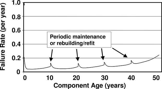
Figure 7.4 A bathtub curve showing impact of periodic rebuilding and refitting.
Figure 7.3 identifies three different failure periods of the device’s lifetime. These are:
1. Break-in period. Failure rate for equipment is often higher for new equipment, as shown in Figure 7.3. Flaws in manufacturing, or installation, lead to quick failure of the device once placed in service.
2. Useful lifetime. Once the break-in period is past, there is a lengthy period when the device is performing as designed and failure rate is low, during which the design balance of all of its deterioration rates is achieving its goal. During this period, for many types of equipment, the failure rates due to “natural causes” (deterioration due to chronological aging and service stress) may be so low that the major causes of failure are abnormal events.
3. Wear-out period. At some point, the failure rate begins to increase, due to the cumulative effect of time, service stress, and abnormal events. From this point forward it increases with time, reaching the high double-digit percentages at some point.
Often periodic maintenance, rebuilding or refitting, can “extend” lifetime or lower expected failure rate, as shown in Figure 7.4. This concept applies only to units designed for or conducive to service (i.e., this applies to breakers, perhaps, but not overhead conductors). Here, the unit is serviced every ten years or so. Note however, that failure rate still increases over time, just at a lower rate of increase, and that these periodic rebuilds create their own temporary “infant mortality” increases in failure rate.
Failure Rate Always Increases With Age
All available data indicates that inevitably, failure rate increases with age in all types of power system equipment. Figure 7.5 shows data on the failure rate of underground equipment for a utility in the northeast United States, all of which is qualitatively similar to the failure performance seen on all equipment, in any power system.
Failure rate escalation characteristics
Figure 7.6 illustrates how the rate of increase of failure rate over time can exhibit different characteristics. In some cases the failure rate increases steadily over time (the plot is basically a straight line). In other cases the rate of increase increases itself – failure rate grows exponentially with a steadily increasing slope. In yet other cases, the rate climbs steeply for a while and then escalation in failure rate decreases – a so-called “S” shaped curve. Regardless, the key factor is that over time, failure rate always increases.
Eventually the failure rates become quite high
Figure 7.7 is data representing a large population in an actual and very representative electric utility aging equipment investigation done in the late 1990s. Note that the failure rates for all three types of equipment shown eventually reach values that indicate failure within 5 years is likely (rates in the 15 – 20% range). In some cases failure rates reach very high levels (80% -failure in the next year or so is almost a certainty. To power system engineers and managers who have not studied failure data, these values seem startlingly high.3 However, these are typical for power system equipment – failure rates do reach values of 15%, 25% and eventually, 80%. But these dramatically high values are not significant in practice, as will be discussed below, because few units “live” long enough to become that old. What really impacts a utility is the long period at the end of useful lifetime and beginning of the wear-out period when failure rate begins to rise, slowly at first, but inevitably, to two to five times normal (useful lifetime) rates.
3 In many cases the older age/high failure rate portions of a curve fitted to a utility’s data are not statistically sound. Perhaps there was only one unit or one failure of a unit older than 50 years in all the data. Fitting a curve to that data and then extending it out to 100 years provides questionable estimates of failure rate in the 65+year range. Here, there were sufficient old units, and failures, to provide statistically significant sample of old units and trends which their failure rate follows in this time frame.
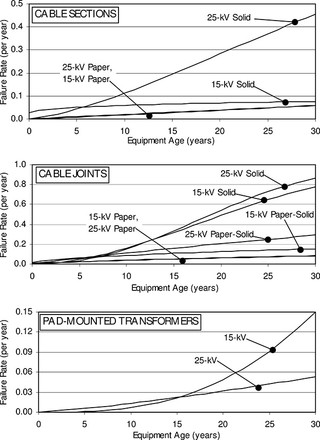
Figure 7.5 Data on failure rates as a function of age, for various types of underground equipment in a utility system in the northeastern United States. Equipment age in this case means, “time in service.” Equipment of different voltage classes can have radically different failure characteristics, but in all cases failure rate increases with age.
7.4 IMPACT OF ESCALATING FAILURE RATES
What Do Aging Utility Equipment Bases Really Look Like?
The paragraph above stated that the very high failures rates reached after 50 years or more (see Figure 7.7) make relatively little impact on a utility’s cost or service quality. The reason is that very few units survive to be so old, so there are few units that have such very high failure rates.
Example 1: A Typical Failure Rate Escalation and Its
Impact on the Installed Equipment Base
Figure 7.6 illustrates a very simple example that will begin this section’s quantitative examination of failure, installed base characteristics, and overall impact on the utility. In this example, the group of 100,000 service transformers is installed at one instant, a rather unrealistic assumption but one that has no impact on the conclusions that this example will draw.
As a group, this set of 100,000 units has the statistical failure rate characteristic shown in the top part of Figure 7.6. That plot gives the probability that an operating unit of any particular age will fail in the next 12 months of service. In this case there is no high break-in-period (infant mortality) failure rate. The base rate during normal lifetime begins at 1.5% per year, rising to 2.5% by year 24, 6.6% by year 30, and to 9% annually by age 40. This curve is representative of actual service transformer failure rate curves (see bottom of Figure 7.6), if noticeably more extreme than is typical for electric utility equipment.
The bottom diagram in Figure 7.6 shows, as a function of age, the percent of the 100,000 units installed in year zero that can be expected to remain in service each year as units fail according to the expectation defined by the top curve. In year one, 1.5% of the units’ fail, meaning 99% are in service at the beginning of year two. At the end of a decade, 85% are still in service.
The failure rate is initially 1.5%, increasing slightly above that value each year. Despite this rise, only 15% of the units (ten times 1.5-%) fail in the first decade. The reason is that the number of initial units left to fail decreases each year – there are only 985,000 units left at the end of the first year, etc., so 1.5% is not exactly 1,500. The number of actual failures decreases slightly each year for the first decade, to a low of only 1,440 failures in year ten, because the number of units remaining to fail drops faster than the failure rate increases.
At the end of 20 years, 71% of the units remain, and at the end of thirty, only 53% remain. The 50% mark is reached at 32 years. By the end of year 50, failure rate has escalated to more than 15%, but only a paltry 10.3% of the original units remain. Only 500 (.7%) make it to year 60. Fewer than two are expected to be in service by year 70, when failure rate has escalated to 50%. The average unit ends up providing 43.8 years of service before failure.
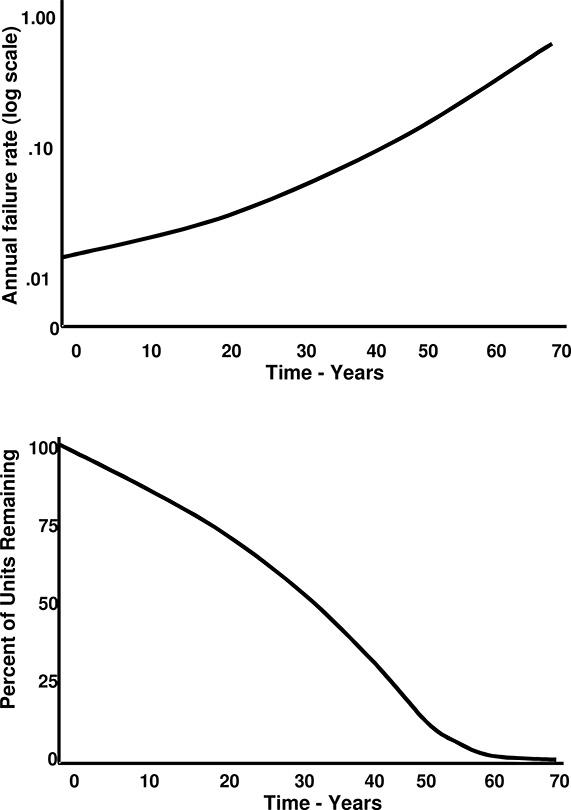
Figure 7.6 Top, failure rates as a function of age for a group of 100,000 service transformers installed in one year. Bottom, the percent remaining of the original group as a function of time.

Figure 7.7 Number of failures occurring each year in the population that originally numbered 100,000 units.
Failures in intermediate years are the real culprit
The very high failure rates that develop after five or six decades of service make little real impact on the utility’s quality of service. Units that are 70 years old have a 50 percent likelihood of failing in the next year, but as shown above, there are only two units out of every 100,000 that make it to that age – essentially an anomaly in the system. They are not going to make a big impact on utility operations.
Instead, the high impact failure levels that would plague a utility operating this equipment would be caused by failures at intermediate age, even though the failure rate in that age range is far lower. Figure 7.7 shows the number of units that fail each year in this example. As mentioned earlier, the number of failures is initially 1,500 units per year and the count actually drops slightly during the first decade as the product (failure rate x number of units remaining) decreases slightly. The number of failures peaks in year 44, with 2,576 expected failures. Thereafter, even though the failure rate keeps increasing every year, the number of remaining units this rate applies to is so low, that the net number of failures decreases rapidly.
Failure-Count Diagrams
Figure 7.7 is a very interesting and significant diagram, because it has another interpretation or use: this is a plot of contribution to failure by age of transformer for any utility system built with this type of unit, regardless of when they were installed. The curve’s shape shows, in relative terms, how much transformers of a particular age contribute to the overall installed base’s failure rate.
In the example used above, all the transformers were installed in the same year, but Figure 7.7 can be applied to cases where a utility installed them in various years. It still has the same meaning, showing the relative contribution to failures of units of various ages. The majority of the failures, nearly two thirds, will be units that are between 15 and 45 years old.
Thus, in this system, with these units, in this year, transformers installed 44 years ago contribute the most to the utility’s annual failure count for service transformers. Given only that the utility added the same number of units each year in the past, this will always be the case. Ten years from now 44-year-old units will be those giving it the most problems, then, only assuming that, 34 years earlier, the same number were installed as 44 years ago. In a system that addsa constant number of units annually in the past, it will always be 44-year-old units that are causing the most problems.
Scenarios involving replacement
In the example given above, units that fail are not replaced. This is not representative of an actual utility situation. In the operation of any utility system, failed units are replaced, the replacements are newer, and thus a more complicated situation will develop. In a “failures are replaced” scenario, in year one, the 1,500 units that fail are replaced with new units so the system of 100,000 goes into the following year (number two year) with most two-year-old units but 1,500 one-year-old units. The following year, a portion of the two-year-old and one-year-old units fail and are replaced with new, etc. Over time, a range of ages from a few new to many old will develop, even though initially all were installed at the same time. Add to this the fact that in real utility systems the units are not installed all at once but over time, and the distribution of ages and the failure-rate over time trends become quite complicated to track and predict. This will be the subject of later chapters and the model discussed in Appendix A. Regardless, the point here is that no matter when they are installed, really old equipment is usually not the equipment causing the most concern to the utility. It will be equipment in “middle age,” which might be usefully defined as in that period when
(number that have survived until now) × (failure rate for this age)
is at a maximum, that matter most. This is significant, for it means that aging infrastructure programs should focus on reducing failure rate in this period rather than for older equipment: life extension programs should begin earlier, not later.
Example 2: A More “Real World” Case
As noted above, Example 1 did not provide for replacement of units when they fail, but tracking only the survivors of that initial batch of 100,000 units. Example 2 builds on Example 1, using the same type of service transformers. It:
1. Assumes, as before, 100,000 units installed in year 0.
2. Assumes a period of 70 years.
3. Assumes the failed units are replaced immediately with new ones, keeping the overall count at 100,000.
4. Assumes these new units follow the same failure rate curve as the original units.
This is a more realistic example, as it represents what a utility has to do – keep the same number of units in service, replacing failed units when they fail.4 The major change in the overall equipment base and its interaction with failures in this example is that replacement units can fail, too.
What does this installed equipment base look like with respect to age distribution of units in service, average failure rate, and failure count? Figure 7.8 shows the distribution of ages of the 100,000 units in the system after 70 years. In year 1 (the first year) 1,500 units failed, and were replaced with new units which are now 69 years old. Those 1,500 units failed with the same characteristic trend as the original set, meaning that 1.5-%, or 23, failed and were replaced in their first year of service (year 68). In that year, 1,489 of the original 100,000 units failed (1.5% of the 998,500 remaining original units). Thus, a total of 1,512 replacement units were installed in year 2. They began to fail along the same trend as the original units, so that in year 3 there were failures of units that had been installed in years 0, 1, and 2, etc.
The net result, when all of these replacements, and replacements for replacements that failed, etc., are added up, is that the utility had to install about 60,000 additional replacement units during the 70-year-period. And, following the failure count contributions of Figure 7.7, most of those replaced were of “middle aged transformers” – those in the 15 –45 year old range. Thus, Figure 7.8 gives the relative age of units replaced by the utility over the course of its annual O&M in each year.
4 The fact that this example assumes the system is created from scratch in year zero makes no impact on the results given here. As shown earlier, by year 70 only 2 of the original units are left. The population consists of units that have been replaced, and in some cases, failed and replaced again. As a result after 70 years there is only an insignificant “start effect” involved in the data – the model’s results in year 70 represent a fairly stable look at what year-to-year operation for the utility would be with respect to service transformers.
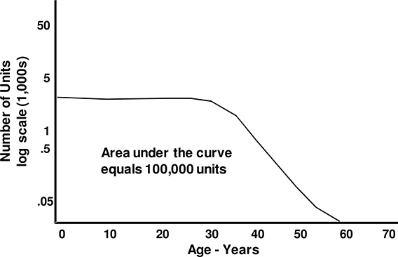
Figure 7.8 Distribution of ages of units in the Example 2 system, 100,000 units that have been replaced as they failed over the last 70 years.
Figure 7.8 shows the resulting equipment bases distribution of transformer ages, after 70 years. It has nearly an even distribution of transformers from age 0 (new) to 30 years. Thus, despite the escalating failure rate as transformers near age 30, 30 years can be considered a reasonable definition of the “useful life” of these units. At about 35 years the count takes a rapid plunge – this is the period (about 35 years in service) during which the bulk of failure counts occur (see Figure 7.4), and thus the age when a good deal of replacements had to be made.
In this system, the average unit in service is 22 years old. However, due to the escalation of failure rates as units age, those older than the average contribute a good deal more to the average failure rate. The entire population has an average failure rate of 3.15%, or more than twice that of new units. This corresponds to the failure rate of a unit that is 29 years old (see Figure 7.8, top).
Replacement policy analysis
Suppose this utility decided to replace all units when they reached fifty years in service. It would have to replace only about 75 units annually – not a tremendous cost, particularly considering the units will have to be replaced pretty soon, anyway (they will most likely fail in a few years, at that age). However, the impact on the overall failure rate is insignificant, making no real difference in the average age or failure rates for the total population. The high impact on annual failure count comes from units that are aged 25 to 45 years, because there are so many of them. Replacement at age 50 gets to the units after too many have failed.
Replacement of units at age 40 has a far different effect. First, nearly 1000 units a year have to replaced, so the annual cost is roughly 12 times that of a 50-year replacement policy. But, noticeable portions of unexpected failures are avoided. The average failure rate drops to 2.6% (from 3.1%), a reduction in unexpected failures of nearly 20%, wrought by replacement on only 1% of the units in the system annually.
Average age of a unit under this policy falls to less than 18 years (if all units were replaced at age 40 and none failed until that age, the average age of units in service would be exactly 20 years). The population’s average failure rate of 2.6% is equivalent to the failure rate of a 25-year-old unit. Whether this policy makes economic sense or not is something for management to weigh in its evaluation of how best to spend the (always-limited) monies it has for system improvements. That will be discussed in Chapter 12.
7.5 SUMMARY OF KEY POINTS
All equipment installed in an electric system will eventually fail and need to be replaced. Key points brought up in this chapter are:
1. Failure is caused by deterioration, due to the effects of age, service, and infrequent but stressful abnormal events.
2. This deterioration eventually leads to failure.
3. Due to efficient design of most equipment, a unit that is near failure from one area of deterioration is probably fairly “shot” in other areas, too.
4. Regardless of equipment type, the failure increases, as a unit grows older.
5. For an installed base of equipment, the bulk of failures will come not from very old equipment but from “middle aged” equipment.
6. In all cases, due to failure rate escalation with age, the equivalent failure rate of an installed equipment base will correspond to a much older age than the average age of the equipment.
7. “Early replacement” policies can be worked out to determine if and how equipment should be replaced at some specific age (e.g., 40 years) and what that impact that would have on the net failure rate of the equipment base.
REFERENCES AND BIBLIOGRAPHY
P. F. Albrecht and H. E Campbell, “Reliability Analysis of Distribution Equipment Failure Data,” EEI T&D Committee Meeting, January 20, 1972.
R. E. Brown, and J. R. Ochoa, “Distribution System Reliability: Default Data and Model Validation,” paper presented at the 1997 IEEE Power Engineering Society Summer Meeting, Berlin.
J. B. Bunch, H.I Stalder, and J.T. Tengdin, “Reliability Considerations for Distribution Automation Equipment,” IEEE Transactions on Power Apparatus and Systems, PAS-102, November 1983, pp. 2656 - 2664.
“Guide for Reliability Measurement and Data Collection,” EEI Transmission and Distribution Committee, October 1971, Edison Electric Institute, New York.
Institute of Electrical and Electronics Engineers, Recommended Practice for Design of Reliable Industrial and Commercial Power Systems, The Institute of Electrical and Electronics Engineers, Inc., New York, 1990.
A. D. Patton, “Determination and Analysis of Data for Reliability Studies,” IEEE Transactions on Power Apparatus and Systems, PAS-87, January 1968.
N. S. Rau, “Probabilistic Methods Applied to Value-Based Planning,” IEEE Transactions on Power Systems, November 1994, pp. 4082 - 4088.
A. J. Walker, “The Degradation of the Reliability of Transmission and Distribution Systems During Construction Outages,” Int. Conf. on Power Supply Systems. IEEE Conf. Publ. 225, January 1983, pp. 112 - 118.
H. B. White, “A Practical Approach to Reliability Design,” IEEE Transactions on Power Apparatus and Systems, PAS-104, November 1985, pp. 2739 - 2747.