
3 Customer Demand for Power and Reliability of Service
3.1 THE TWO Qs: QUANTITY AND QUALITY OF POWER
Electric consumers require power, whether delivered from the utility grid or generated locally by distributed sources, in order to help accomplish the uses for which they need energy. Their need for electric power, and the value they place upon its delivery to them, has two interrelated but fundamentally separate dimensions. These are the two Qs: Quantity, the amount of power needed, and Quality, the most important aspect of which is usually dependability of supply (reliability of power supply, or availability as it is often called). The relative importance of these two features varies from one consumer to another depending on their individual needs, but each consumer finds value in both the amount of power he obtains, and its availability as a constant, steady source that it will be there whenever needed.
This chapter discusses demand and use of electric power as seen from the customer’s standpoint: the utility’s job is to satisfy consumer needs as fully as possible within reasonable cost constraints. Cost is very much an important aspect to consumers too, so both the utility and the consumer must temper their plans and desires with respect to power and reliability based on real world economics. Consumers do not get everything they want; only what they are willing to pay for.
Utilities should not aim to provide flawless service, which would be prohibitively expensive, but instead aim to provide the highest level possible within economic constraints of the customers’ willingness to pay.
This chapter begins, in Section 3.2, with a discussion of consumer use of electricity and includes the quantity of electric demand as seen from an “end-use” perspective. It continues with how demand varies as a function of consumer type and end-use, and how power demand is represented in electric system studies using load curves and load duration curves. Section 3.3 then discusses reliability and availability as seen by the customers and ways this can be characterized and studied. Section 3.4 briefly reviews Two-Q analysis and planning concepts and their application to customer load analysis. Finally, Section 3.5 provides a summary of key points.
3.2 ELECTRIC CONSUMER NEED FOR QUANTITY OF POWER
People and businesses buy power because they want the products that electrical use can provide
No consumer actually wants the electric energy itself. Consumers want the products it can provide - a cool home in summer, hot water on demand, compressed air for manufacturing, electronic robotic factory control, cold beer in the ‘fridge and football on color TV. Electricity is only an intermediate means to some end-use.
These different goals and needs are called end-uses, and they span a wide range of applications. Some end-uses are unique to electric power (the authors are not aware of any manufacturer of natural gas powered TVs, stereos, or computers). For many other end-uses, electricity is only one of several possible energy sources (water heating, home heating, cooking, or clothes drying). In many other end-uses, electricity is so convenient that it enjoys a virtual monopoly, even though there are alternatives, e.g., gasoline-powered refrigerators, and natural gas for interior lighting and for air conditioning.
Each end-use is satisfied through the application of appliances
Lighting was the first and is still the largest single category or end use of power in many utility systems. A wide range of illumination devices are used, including incandescent bulbs, fluorescent tubes, sodium vapor, high-pressure monochromatic gas-discharge tubes, and in special cases, lasers. Each type of lighting device has differences from the others that give it an appeal to some consumers or for certain types of applications. Regardless, each requires electric power to function, creating an electric load when it is activated.

Figure 3.1 Electric peak demand of a utility in the southeastern United States broken down by consumer class and within the residential class, by contribution to peak for the major uses for which electricity is purchased at time of peak by the residential class.
Similarly, for other end-uses, such as space heating, there are various types of appliances, each with advantages or disadvantages in initial cost, operating efficiency, reliability and maintenance, noise and vibration, or other aspects. Buildings can be heated by heat pumps of various types and efficiencies, circulating hot water, or simple resistive heat. Each produces an electric load when used to produce heat for a home or business. Each has advantages (resistive heaters are cheap to buy, heat pumps use the least power of all heater types) and disadvantages (resistive heaters are inefficient, heat pumps are expensive to buy).
Consumer Classes
Different types of consumers purchase electricity. About half of all electric power is used in residences, which vary in the brands and types of appliances they own, and their daily activity patterns. Another fourth is consumed by commercial businesses both large and small, that buy electricity, having some similar end-uses to residential consumers (heating and cooling, and illumination), but that have many needs unique to commercial functions (cash register/inventory systems, escalators, office machinery, neon store display lighting, parking lot lighting). Finally, industrial facilities and plants buy electricity to power processes such as pulp heating, compressor and conveyor motor power, and a variety of manufacturing applications. As a result, the load on an electric system is a composite of many consumer types and appliance applications. Figure 3.1 shows this breakdown of the peak electrical load for a typical power system by consumer class and end-use category within one class.
Appliances Use Electric Power to Satisfy End-Use Demand
The term load refers to the electrical demand of a device connected to and drawing power from the electric system in order to accomplish some task, e.g., opening a garage door, or converting that power to some other form of energy, such as a light. Such devices are called appliances, whether they are a commonly regarded household item, e.g., a refrigerator, lamp, garage door opener, paper shredder, electric fence to keep cattle confined, etc. To the consumer, these appliances convert electricity into the end product. But the electric service planner can turn this relation around and view an appliance (e.g., a heat pump) as a device for transforming a demand for a particular end-use - warm or cool air - into electric load.
The level of power they need usually rates electrical loads, measured in units of real volt-amperes, called watts. Large loads are measured in kilowatts (thousands of watts) or megawatts (millions of watts). Power ratings of loads and T&D equipment refer to the device at a specific nominal voltage. For example, an incandescent light bulb might be rated at 75 watts and 1,100 lumens at 120 volts, at which voltage it consumes 75 watts and produces 1,100 lumens of light. If provided with less voltage, its load (and probably its light output) will fall. By this definition, an electric vehicle (EV) such as a Chevrolet Volt is an appliance. It converts electric power drawn from the grid into an end use (personal transportation – the ability to move from place to place). EVs are one example of how and why electric energy consumption and the value society as a whole sees from utility service continues to grow.
Load Curves and Load Curve Analysis
The electric load created by any one end-use usually varies as a function of time. For example, in most households, demand for lighting is highest in the early evening, after sunset but before most of the household members have gone to bed. Lighting needs may be greater on weekends, when activity often lasts later into the evening, and at times of the year when the sun sets earlier in the day. Some end-uses are quite seasonal. Air-conditioning demand generally occurs only in summer, being greatest during particularly hot periods and when family activity is at its peak, usually late afternoon or very early evening. Figure 3.2 shows how the demand for two products of electric power varies as a function of time.

Figure 3.2 End-use demand. Right, average demand for BTU of cooling among houses in one of the authors’ neighborhoods on a typical weekday in June. Left, lighting lumens used by a retail store on a typical day in June.

Figure 3.3 Electric demand for each class varies hourly and seasonally, as shown here, with a plot of average coincident load for residential users in central Florida.
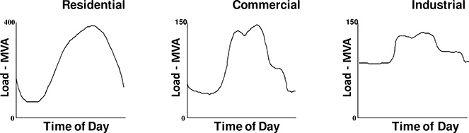
Figure 3.4 Different consumer classes have different electrical demand characteristics, particularly with regard to how demand varies with time. Here are summer peak day load curves for the three major classes of consumer from the same utility system.
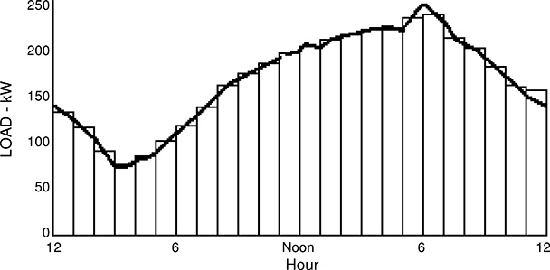
Figure 3.5 Demand on an hourly basis (blocks) over 24 hours, and the actual load curve (solid black line) for a feeder segment serving 53 homes. Demand measurement averages load over each demand interval (in this case each hour) missing some of the detail of the actual load behavior. In this case the actual peak load (263 kW at 6 PM) was not seen by the demand measuring, which “split the peak,” averaging load on an hourly basis and seeing a peak demand of only 246 kW, 7% lower. As will be discussed later in this chapter, an hourly demand period is too lengthy for this application.
The result of this varying demand for the products of electricity application, is a variation in the demand for power as a function of time. This is plotted as a load curve, illustrated in Figure 3.3. Typically, the values of most interest to the planners are the peak load (maximum amount of power that must be delivered). This defines directly or indirectly, the capacity requirements for equipment; the minimum load and the time it occurs; the total energy, area under the curve that must be delivered during the period being analyzed; and the load value at the time of system peak load.
Consumer Class Load Curves
While all consumers differ in their electrical usage patterns, consumers within a particular class, such as residential, tend to have broadly similar load curve patterns. Those of different classes tend to be dissimilar in their demand for both quality and quantity and the time of day and year when their demand is highest. Therefore, most electric utilities distinguish load behavior on a class-by-class basis, characterizing each class with a “typical daily load curve,” showing the average or expected pattern of load usage for a consumer in that class on the peak day, as shown in Figure 3.4. These “consumer class load curves” describe how the demand varies as a function of time. While often an entire 8,760-hour record for the year is available, usually only key days – perhaps one representative day per season – are used for studies.
The most important points concerning the consumers’ loads from the distribution planner’s standpoint are:
1. Peak demand and its time and duration
2. Demand at time of system peak
3. Energy usage (total area under the annual load curve)
4. Minimum demand, its time and duration
Details of Load Curve Measurement
Demand and demand periods
“Demand,” as normally used in electric load analysis and engineering, is the average value of electric load over a period of time known as the demand interval. Very often, demand is measured on an hourly basis as shown in Figure 3.5, but it can be measured on any interval basis - seven seconds, one minute, 30 minutes, daily, and monthly. The average value of power during the demand interval is given by dividing the kilowatt-hours accumulated during the demand interval by the length of the interval. Demand intervals vary among power companies, but those commonly used in collecting data and billing consumers for “peak demand” are 15, 30, and 60 minutes. Load curves may be recorded, measured, or applied over some specific time. For example, a load curve might cover one day. If recorded on an hourly demand basis, the curve consists of 24 values, each the average demand during one of the 24 hours in the day, and the peak demand is the maximum hourly demand seen in that day. Load data is gathered and used on a monthly basis and on an annual basis.
Load factor
Load factor is the ratio of the average to the peak demand. The average load is the total energy used during the entire period (e.g., a day, a year) divided by the number of demand intervals in that period (e.g., 24 hours, 8,760 hours). The average is then divided by the maximum demand to obtain the load factor:
Load factor = kWh/Hrs/Peak kW = Average kW/Peak kW (3.1)
= KWhr/(Peak kW x Hr) (3.2)
Load factor gives the extent to which the peak load is maintained during the period under study. A high load factor means the load is at or near peak a good portion of the time.
Load Duration Curves
A convenient way to study load behavior is to order the demand samples from greatest to smallest, rather than as a function of time, as in Figure 3.6. The two diagrams consist of the same 24 numbers, in a different order. Peak load, minimum load, and energy (area under the curve) are the same for both.
Load duration curve behavior will vary as a function of the level of the system. Load duration curves for small groups of consumers will have a greater ratio of peak to minimum than similar curves for larger groups. Those for very small groups (e.g., one or two consumers) will have a pronounced “blockiness,” consisting of plateaus – many hours of similar demand level (at least if the load data were sampled at a fast enough rate). The plateaus correspond to combinations of major appliance loads. The ultimate “plateau” would be a load duration curve of a single appliance, for example a water heater that operated a total of 1,180 hours during the year. This appliance’s load duration curve would show 1,180 hours at its full load, and 7,580 hours at no load, without any values in between.

Figure 3.6 The hourly demand samples in a 24-hour load curve are reordered from greatest magnitude to least to form a daily load duration curve.
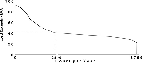
Figure 3.7 Annual load duration curve for a proposed commercial site with a 90 kW peak demand, from a DG reliability study in which three 40 kW distributed generators will be used to provide the power. As shown here, the demand exceeds 40 kW, the capacity of one unit, 2,800 hours a year. During those 2,800 hours, service can be obtained only if two or more units are operating. Information like this helps planners determine the equipment needs of power systems and project future operating costs.
Annual load duration curves
Most often, load duration curves are produced on an annual basis, reordering all 8,760 hourly demands (or all 35,040 quarter hour demands if using 15-minute demand intervals) in the year from highest to lowest, to form a diagram like that in Figure 3.7. The load shown was above 26 kW (demand minimum) 8,760 hours in the year, never above 92 kW, but above 40 kW for 2,800 hours. basis, an often important aspect of siting for facilities, including DG (Willis, 1996).
Most often, load duration curves are produced on an annual basis, reordering all 8,760 hourly demands (or all 35,040 quarter hour demands if using 15-minute demand intervals) in the year from highest to lowest, to form a diagram like that in Figure 3.7. The load shown was above 26 kW (demand minimum) 8,760 hours in the year, never above 92 kW, but above 40 kW for 2,800 hours.
Load Duration Curves Do Not Provide Detailed Load Behavior Data
The load duration curve is a traditional tool used to represent the larger aspects of behavior of electric load. It developed prior to WWI and used in conjunction with other pre-computer era analytical tools such as break-point analysis for generation planning and K-factor analysis in distribution planning. In the 21st century, a load duration curve provides a useful way to summarize the major aspects of a utility’s demand behavior y, but does not provide the information needed for modern planning methods, nor put it in a form compatible with modern analytical system engineering tools. It is not a tool recommended by the authors for anything more than screening studies.
The major limitation of the load duration curve is that it does not provide information on the order in time of the load values it plots. The 2,800 hours when load is above 40 kW, shown in Figure 3.7, could be clustered entirely in the May – September timeframe, or spread evenly through the year as 7.7 hour periods every day. Such details are important both for determining the type and operating cost of the DG units, and for applying modern IRP methods that would seek to use load control and other means to maximize energy efficiency at the site.
Spatial Patterns of Electric Demand
An electric utility must not only produce or obtain the power required by its consumers, but also must deliver it to their locations. Electric consumers are scattered throughout the utility service territory, and thus the electric load can be thought of as distributed on a spatial basis as depicted in Figure 3.9. Just as load curves show how electric load varies as a function of time, (and can help identify when certain amounts of power must be provided), so has Spatial Load Analysis been used since its development in the 1970s (Scott, 1972) to identify where load is located and how much capacity is needed in each locality.
The electric demand in an electric utility service territory varies as a function of location depending on the number and types of consumers in each locality, as shown by the load map in Figure 3.9. Load densities in the heart of a large city can exceed 1 MW/acre, but usually average about 5 MW per square mile over the entire metropolitan area. In sparsely populated rural areas, farmsteads can be as far as 30 miles apart, and load density as low as 75 watts per square mile.

Figure 3.8 Left, map showing types of consumer by location for a small city. Right, map of electric demand for this same city.
Regardless of whether an area is urban, suburban, or rural, electric load is a function of the types of consumers, their number, their uses for electricity, and the appliances they employ. Other aspects of power system performance, including capability, cost, and reliability, can also be analyzed on a location- basis, an often important aspect of siting for facilities, including DG (Willis, 1996).
3.3 ELECTRIC CONSUMER NEED FOR QUALITY OF POWER
As mentioned in this chapter’s introduction, a central issue in customer value of service analysis is matching availability and power quality against cost. T&D systems with near perfect availability and power quality can be built, but their high cost will mean electric prices the utility customers may not want to pay, given the savings an even slightly less reliable system would bring. All types of utilities have an interest in achieving the correct balance of quality and price. The traditional, franchised monopoly utility, in its role as the “electric resource manager” for the customers it serves, has a responsibility to build a system whose quality and cost balances its customers’ needs. A competitive retail distributor of power wants to find the best quality-price combination - only in that way will it gain a large market share.
While it is possible to characterize various power quality problems in an engineering sense, characterizing them as interruptions, voltage sags, dips, surges, or harmonics, the customer perspective is somewhat different. Customers are concerned with only two aspects of service quality:
1. They want power when they need it.
2. They want the power to do the job.
If power is not available, neither aspect is provided. However, if power is available, but quality is low, only the second is not provided.
Assessing Value of Quality by Studying the Cost of a Lack of It
In general, customer value of reliability and service quality are studied by assessing the “cost” that something less than perfect reliability and service quality creates for customers. Electricity provides a value, and interruptions or poor power quality decrease that value. This value reduction - cost - occurs for a variety of reasons. Some costs are difficult, if not impossible to estimate: re-scheduling of household activities or lack of desired entertainment when power fails1, or flickering lights that make reading more difficult.
But often, very exact dollar figures can be put on interruptions and poor power quality including food spoiled due to lack of refrigeration; wages and other operating costs at an industrial plant during time without power; damage to product caused by the sudden cessation of power; lost data and “boot up” time for computers; equipment destroyed by harmonics; and so forth. Figure 3.9 shows two examples of such cost data.
1 No doubt, the cost of an hour-long interruption that began fifteen minutes from the end of a crucial televised sporting event, or the end of a “cliffhanger” movie, would be claimed to be great.

Figure 3.9 Left, cost of a week-day interruption of service to a pipe rolling plant in the southeastern United States, as a function of interruption duration. An interruption of any length costs about $5,000 - lost wages and operating costs to unload material in process, bring machinery back to “starting” position and restart - and a nearly linear cost thereafter. At right, present worth of the loss of life caused by harmonics in a 500 horsepower three-phase electric motor installed at that same industrial site, as a function of harmonic voltage distortion.
Value-Based Planning
To be of any real value in utility planning, information of the value customers put on quality must be usable in some analytical method that can determine the best way to balance quality against cost. Value-based planning (VBP) is such a method: it combines customer-value data of the type shown in Figure 3.9 with data on the cost to design the T&D system to various levels of reliability and power quality, in order to identify the optimum balance. Figure 3.10 illustrates the central tenet of value-based planning. The cost incurred by the customer due to various levels of reliability or quality, and the cost to build the system to various levels of reliability, are added to get the total cost of power delivered to the customer as a function of quality.2 The minimum value is the optimum balance between customer desire for reliability and aversion to cost. This approach can be applied for only reliability aspects, i.e., value-based reliability planning, or harmonics, or power quality overall. Generally, what makes sense is to apply it on the basis of whatever qualities (or lack of them) impact the customer - interruptions, voltage surges, harmonics, etc., in which case it is comprehensive value-based quality of service planning.
2 Figure 3.10 illustrates the concept of VBP. In practice, the supply-side reliability curves often have discontinuities and significant non-linearities that make application difficult. These and other details will be discussed in Chapter 5.
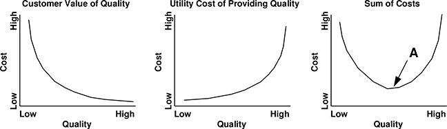
Figure 3.10 Concept of value-based planning. The customer’s cost due to poorer quality (left) and the cost of various power delivery designs with varying levels of quality (center) are computed over a wide range. When added together (right) they form the total cost of quality curve, which identifies the minimum cost reliability level (point A).
Cost of Interruptions
The power quality issue that affects the most customers, and which receives the most attention, is cessation of service often termed “service reliability.” Over a period of several years, almost all customers served by any utility will experience at least one interruption of service. By contrast, a majority will never experience serious harmonics, voltage surge, or electrical noise problems. Therefore, among all types of power quality issues, interruption of service receives the most attention from both the customers and the utility. A great deal more information is available about cost of interruptions than about cost of harmonics or voltage surges.
Voltage Sags Cause Momentary Interruptions
The continuity of power flow does not have to be completely interrupted to disrupt service: If voltage drops below the minimum necessary for satisfactory operation of an appliance, power has effectively been “interrupted” as illustrated in Figure 3.11. For this reason many customers regard voltage dips and sags as momentary interruptions - from their perspective these are interruptions of the end-use service they desire, if not of voltage.
Much of the electronic equipment manufactured in the United States, as well as in many other countries, have been designed to meet or exceed the CBEMA

Figure 3.11 Output of a 5.2 volt DC power supply used in a desktop computer (top) and the incoming AC line voltage (nominal 113 volts). A voltage sag to 66% of nominal causes power supply output to cease within three cycles.

Figure 3.12 CBEMA curve of voltage deviation versus period of deviation, with the sag shown in Figure 3.11 plotted (black dot).
(Computer and Business Equipment Manufacturer’s Association) recommended curves for power continuity, shown in Figure 3.12. If a disturbance’s voltage deviation and duration characteristics are within the CBEMA envelope, then normal appliances should operate normally and satisfactorily.
However, many appliances and devices in use will not meet this criterion at all. Others will fail to meet it under the prevailing ambient electrical conditions (i.e., line voltage, phase unbalance power factor, and harmonics may be less than perfect).
The manner of usage of an appliance also affects its voltage sag sensitivity. The voltage sag illustrated in Figure 3.11 falls just within the CBEMA curve, as shown in Figure 3.12. The manufacturer probably intended for the power supply to be able to withstand nearly twice as long a drop to 66% of nominal voltage before ceasing output. However, the computer in question had been upgraded with three times the standard factory memory, a second and larger hard drive, and optional graphics and sound cards, doubling its power usage and the load on the power supply. Such situations are common and means that power systems that deliver voltage control within recommended CBEMA standards may still provide the occasional momentary interruption.
For all these reasons, there are often many more “momentary interruptions” at a customer site than purely technical evaluation based on equipment specifications and T&D engineering data would suggest. Momentary interruptions usually cause the majority of industrial and commercial interruption problems. In addition, they can lead to one of the most serious customer dissatisfaction issues. Often utility monitoring and disturbance recording equipment does not “see” voltage disturbances unless they are complete cessation of voltage, or close to it. Many events that lie well outside the CBEMA curves and definitely lead to unsatisfactory equipment operation are not recorded or acknowledged. As a result, a customer can complain that his power has been interrupted five or six times in the last month, and the utility will insist that its records show power flow was flawless. The utility’s refusal to acknowledge the problem irks some customers more than the power quality problem itself.
Frequency and Duration of Interruptions Both Impact Cost
Traditional Power System Reliability Analysis recognizes that service interruptions have both frequency and duration (See Chapter 4). Frequency is the number of times during some period (usually a year) that power is interrupted. Duration is the amount of time power is out of service. Typical values for urban/suburban power system performance in North America are 2.2 interruptions per year with 100 minutes total duration.
Both frequency and duration of interruption impact the value of electric service to the customer and must be appraised in any worthwhile study of customer value of service. A number of reliability studies and value-based planning methods have tried to combine frequency and duration in one manner or another into “one dimension.” A popular approach is to assume all interruptions are of some average length (e.g., 2.2 interruptions and 100 minutes is assumed to be 2.2 interruptions per year of 46 minutes each). Others have assumed a certain portion of interruptions are momentary and the rest of the duration is lumped into one “long” interruption (i.e., 1.4 interruptions of less than a minute, and one 99-minute interruption per year). Many other approaches have been tried (see References and Bibliography). But all such methods are at best an approximation, because frequency and duration impact different customers in different ways. No single combination of the two aspects of reliability can fit the value structure of all customers.
Figure 3.13 shows four examples of the author’s preferred method of assessing interruption cost, which is to view it as composed of two components, a fixed cost (Y intercept) caused when the interruption occurred, and a variable cost that increases as the interruption continues. As can be seen in Figure 3.13, customer sensitivity to these two factors varies greatly. The four examples are:
1. A pipe-rolling factory (upper left). After an interruption of any length, material in the process of manufacturing must be cleared from the welding and polishing machinery, all of which must be reset and the raw material feed set up to begin the process again. This takes about 1/2 hour and sets a minimum cost for an interruption. Duration longer than that is simply a linear function of the plant operating time (wages and rent, etc., allocated to that time). Prior to changes made by a reliability study, the “re-setting” of the machinery could not be done until power was restored (i.e., time during the interruption could not be put to use preparing to re-start once it was over). The dotted line shows the new cost function after modifications to machinery and procedure were made so that preparations could begin during the interruption.
2. An insurance claims office (upper right) suffers loss of data equivalent to roughly one hour’s processing when power fails. According to the site supervisor, an unexpected power interruption causes loss of about one hour’s work as well as another estimated half hour lost due to the impact of any interruption on the staff. Thus, the fixed cost of each interruption is equivalent to about ninety minutes of work. After one-half hour of interruption, the supervisor’s policy is to put the staff to work “on other stuff for a while,” making cost impact lower (some productivity); thus, variable interruption cost goes down. The dotted line shows the cost impact of interruptions after installation of UPS on the computer system, which permits orderly shutdown in the event of an interruption.

Figure 3.13 The author’s recommended manner of assessing cost of interruptions includes evaluation of service interruptions on an event basis. Each interruption has a fixed cost (Y-intercept) and a variable cost, which increases as the interruption continues. Examples given here show the wide range of customer cost characteristics that exist, and that residential costs a generally far less than commercial costs: the scale of the residential curve is 1/1000th of those for the other classes shown. The text gives details on the meaning of solid versus dotted lines and the reasons behind the curve shape for each customer.
3. An acetate manufacturing and processing plant (lower left) has a very non-linear cost curve. Any interruption of service causes $38,000 in lost productivity and after-restoration set-up time. Cost rises slowly for about half an hour. At that point, molten feedstock and interim ingredients inside pipes and pumps begins to cool, requiring a day-long process of cleaning sludge and hardened stock out of the system. The dotted line shows the plant’s interruption cost function after installation of a diesel generator, started whenever interruption time exceeds five minutes.
4. Residential interruption cost function (lower right), estimated by the authors from a number of sources including a survey of customers made for a utility in the northeastern United States in 1992, shows roughly linear cost as a function of interruption duration, except for two interesting features. The first is the fixed cost equal to about eight minutes of interruption at the initial variable cost slope which reflects “the cost to go around and re-set our digital clocks,” along with similar inconvenience costs. The second is a jump in cost between 45 and 60 minutes, which reflect inconsistencies in human reaction to outage, time on questionnaires. The dotted line shows the relation the authors’ uses in their analysis, which makes adjustments thought reasonable to account for these inconsistencies.
This recommended analytical approach, in which cost is represented as a function of duration on a per event basis, requires more information and more analytical effort than simpler “one-dimensional” methods of reliability evaluation. However, advantages are that the method is more sensitive to actual customer needs, and that the results are more credible when used objectively, in justifying utility expenditures and efforts to improve reliability.
Interruption Cost is Lower if Prior Notification is Given
Given sufficient time to prepare for an interruption of service, most of the momentary interruption cost (fixed) and a great deal of the variable cost can be eliminated by many customers. Figure 3.14 shows the interruption cost figures from Figure 3.13 adjusted for “24 hour notification given.” These are much lower than for situations where no notice is given.
Cost of Interruption Varies by Customer Class
Cost of power interruption varies among all customers, but there are marked distinctions among classes, even when cost is adjusted for “size” of load by computing all cost functions on a per kW basis. Generally, the residential class has the lowest interruption cost per kW and commercial has the highest. Table 3.1
Table 3.1 Typical Interruption Costs by Class for Three Utilities - Daytime, Weekday (dollars per kilowatt hour)
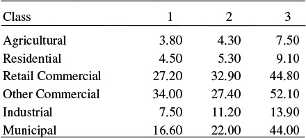
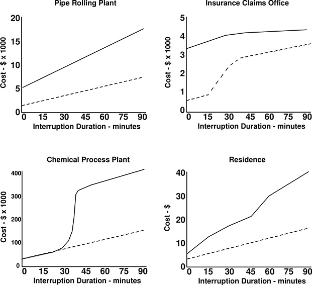
Figure 3.14 If an interruption of service is expected customers can take measures to reduce its impact and cost. Solid lines are the interruption costs (the solid lines from Figure 3.13). Dotted lines show how 24-hour notice reduces the cost impact in each case.
gives the cost/kW of a one-hour interruption of service by customer class, obtained using similar survey techniques for three utilities in the United States:
1. A small municipal system in the central plains,
2. an urban/suburban/rural system on the Pacific Coast and,
3. an urban system on the Atlantic coast.
Cost Varies from One Region to Another
Interruption costs for apparently similar customer classes can vary greatly depending on the particular region of the country or state in which they are located. There are many reasons for such differences. The substantial difference (47%) between industrial costs in utilities 1 and 3 shown in Table 3.14 is due to differences in the type of industries that predominate in each region. The differences between residential costs of the regions shown reflect different demographics and varying degrees of economic health in their respective regions.
Cost Varies among Customers within a Class
The figures given for each customer class in Table 3.1 represent an average of values within those classes as surveyed and studied in each utility service territory. Value of availability can vary a great deal among customers within any class, both within a utility service territory and even among neighboring sites. Large variations are most common in the industrial class, where different needs can lead to wide variations in the cost of interruption, as shown in Table 3.2. Although documentation is sketchy, indications are the major differing factor is the cost of a momentary interruption - some customers are very sensitive to any cessation of power flow, while others are impacted mainly by something longer than a few cycles or seconds.
Cost of Interruption Varies as a Function of Time of Use
Cost of interruption will have a different impact depending on the time of use, usually being much higher during times of peak usage, as shown in Figure 3.15. However, when adjusted to a per-kilowatt basis, the cost of interruption can sometimes be higher during off-peak than during peak demand periods, as shown. There are two reasons. First, the data may not reflect actual value. A survey of 300 residential customers for a utility in New England revealed that customers put the highest value on an interruption during early evening (Figure 3.15). There could be inconsistencies in the values people put on interruptions (data plotted were obtained by survey).
Table 3.2 Interruption Costs by Industrial Sub-Class for One hour, Daytime, Weekday (dollars per kilowatt)

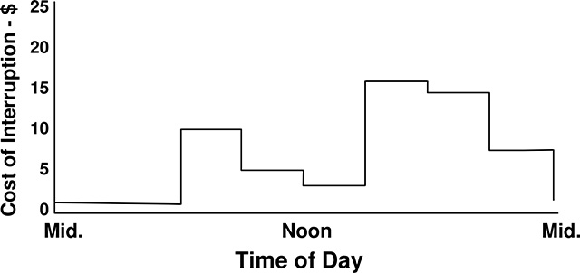
Figure 3.15 Cost of a one-hour interruption as a function of when it occurs, as determined by surveys and interviews with 300 customers of a utility in the northeastern United States, was determined on a three-hour period basis. A high proportion of households in this survey have school age children at home and thus perhaps weighed interruption costs outside of school hours more than during school hours. However, in general, most households rate interruption cost as higher in early morning and early evening.
Recommended Method of Application of Customer Interruption Cost Data
As mentioned earlier, the recommended analytical approach to value-based planning of power delivery includes assessment of customer costs using functions that acknowledge both a fixed cost for any interruption, no matter how brief, and a variable cost as a function of duration. It is also important to acknowledge the differences in value of service among the different customer classes, and the time differences within those customer classes. Often, the cost per kilowatt is highest off-peak. Then, only essential equipment such as burglar alarms, security lighting and refrigeration is operating. These end-uses typically have a high cost of interruption. While it is generally safe to assume that total cost of interruption is highest during peak, the same cannot be assumed about the cost per kilowatt of interruption.
Ideally, reliability and service quality issues should be dealt with using a value-based reliability or power-quality planning method with customer interruption cost data obtained through statistically valid and unbiased sampling of a utility’s own customers (see Sullivan et al.), not with data taken from a reference book, report, or technical paper describing data on another utility system. However, in many cases for initial planning purposes the cost and time of data collection are not affordable.
Figure 3.16 provides a set of costs of typical interruption curves that the author has found often match overall customer values in a system. It is worth stressing that major differences can exist in seemingly similar utility systems, due to cultural and economic differences in the local customer base. These are not represented as average, or “best” for use in value-based planning studies, but they are illustrative of the type of cost functions usually found. They provide a guide for the preparation of approximate data from screening studies and initial survey data.
Cost in Figure 3.16 is given in terms of “one hundred times nominal price.” It is worth noting that in many surveys and studies of interruption cost, the cost per kW of interruption is on the order of magnitude one hundred times the normal price (rate) for a kWh. Generally, if a utility has low rates its customers report a lower cost of interruption than if it has relatively higher rates. No reliable data about why this correlation exists has been forthcoming.3
3 It could be that value of continuity is worth more in those areas where rates are high (generally, more crowded urban areas). However, the authors believe that a good part of this correlation is simply because in putting a value on interruptions, respondents to surveys and in focus groups base their thinking on the price they pay for electricity. Given that a typical residential customer uses roughly 1,000 kWh/month, they may simply be valuing an interruption as about “one tenth of my monthly bill.”
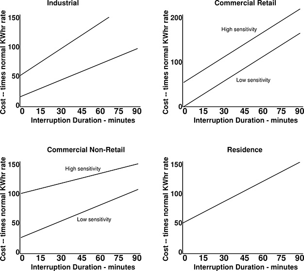
Figure 3.16 Typical interruption cost characteristics for customer classes.
Cost of Surges and Harmonics
Far less information is available on customer costs of harmonics and voltage surges as compared to that available on the cost of interruptions. What data is made available in publications, and most of the reported results and interpretations in the technical literature, were obtained in very customer-specific case studies, most done on a single customer basis. As a result there is very little information available on average of typical costs of voltage surge sensitivity and harmonics sensitivity.
Few customers suffer from voltage dip (voltage problems lasting minutes or hours), surge, harmonics, electrical noise, and similar problems. For this reason most studies of cause, effect, and curve are done on a single-customer or specific area basis. Here, results reported in technical literature are the best guide.
End-Use Modeling of Consumer Availability Needs
The customer-class, end-use basis for analysis of electric usage, discussed in Chapters 2 and 15, provides a reasonably good mechanism for study of the service reliability and power quality requirements of customers, just as it provides a firm foundation for analysis of requirements for the amount of power. Reliability and power quality requirements vary among customers for a number of reasons, but two predominate:
1. End-usage patterns differ. The timing and dependence of customers’ need for lighting, cooling, compressor usage, hot water usage, machinery operation, etc., varies from one to another.
2. Appliance usage differs. The appliances used to provide end-uses will vary in their sensitivity to power quality. For example, many fabric and hosiery manufacturing plants have very high interruption costs purely because the machinery used (robotic looms) is quite sensitive to interruption of power. Others (with older mechanical looms) put a much lower cost on interruptions.
End-use analysis can provide a very good basis for a detailed study of power quality needs. For example, consider two of the more ubiquitous appliances in use in most customer classes: the electric water heater and the personal computer. They represent opposite ends of the spectrum from the standpoint of both amount of power required and cost of interruption. A typical 50-gallon storage electric water heater has a connected load of between 3,000 and 6,000 watts, a standard PC has a demand of between 50 and 150 watts. Although it is among the largest loads in most households, an electric water heater’s ability to provide hot water is not impacted in the least by a one-minute interruption of power. In most cases a one-hour interruption does not reduce its ability to satisfy the end-use demands put on it.4 On the other hand, interruption of power to a computer, for even half a second, results in serious damage to the “product.” Often there is little difference between the cost of a one-minute outage and a one-hour outage.
It is possible to characterize the sensitivity of most end-uses in most customer classes by using an end-use basis. This is in fact how detailed studies of industrial plants are done in order to establish the cost-of-interruption statistics, which they use in VBP of plant facilities and in negotiations with the utility to provide upgrades in reliability to the plant. Following the recommended approach, this requires distinguishing between the fixed cost (cost of momentary interruption) and variable cost (usually linearized as discussed above) on an end-use basis.
4 Utility load control programs offer customers a rebate in order to allow the utility to interrupt power flow to water heaters at its discretion. This rebate is clearly an acceptable value for the interruption, as the customers voluntarily take it in exchange for the interruptions. In this and many other cases, economic data obtained from market research for DSM programs can be used as a starting point for value analysis of customer reliability needs on a value-based planning basis.
A standard end-use model used to study and forecast electric demand can be modified to provide interruption cost sensitivity analysis, which can result in “two-dimensional” appliance end-use models as illustrated in Figure 3.17. Generally, this approach works best if interruption costs are assigned to appliances rather than end-use categories. In commercial and industrial classes different types of appliances within one end-use can have wildly varying power reliability and service needs. This requires an “appliance sub-category” type of an end-use model. Modifications to an end-use simulation program to accommodate this approach are straightforward (see Willis, 1996, Chapter 11), and not only provide accurate representation of interruption cost sensitivity, but produce analysis of costs by time and location, as shown in Figures 3.18 and 3.19.

Figure 3.17 The simulation’s end-use model is modified to handle “two-dimensional” appliance curves, as shown here for a residential electric water heater. The electric demand curve is the same data used in a standard end-use model of electric demand. Interruption cost varies during the day, generally low prior to and during periods of low usage and highest prior to high periods of use (a sustained outage prior to the evening peak usage period would result in an inability to satisfy end-use demand).

Figure 3.18 Result of a power quality evaluation, using an end-use model. Top: the daily load curve for single family homes segmented into four interruption-cost categories. High-cost end-uses in the home are predominantly digital appliances (alarm clocks, computers) and home entertainment and cooking. The bottom figure shows total interruption cost by hour of the day for a one-hour outage - compare to Figure 3.19.
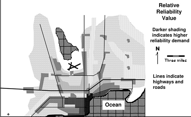
Figure 3.19 Map of average reliability needs computed on a 10-acre small area grid basis for a port city of population 130,000, using a combination of an end-use model and a spatial customer simulation forecast method, of the type discussed in Chapter 15. Shading indicates general level of reliability need (based on a willingness-to-pay model of customer value).
3.4 Two Q Analysis: Quantity and Quality of Power Are Both Important Aspects of Consumer Value
The amount of power used, and the dependability of its availability for use are both key attributes in determining the value of the electric power to each consumer. The values attached to both quantity and quality by most consumers are linked, but somewhat independent of the value attached to the other. In order to demonstrate this, it is worth considering two nearly ubiquitous appliances, which happen to represent opposite extremes of valuation in each of these dimensions: the electric water heater and the personal computer.
A typical residential storage water heater stores about 50 gallons of hot water and has a relatively large connected load compared to most household appliances: about 5,000 watts of heating element controlled by a thermostat. Its contribution to coincident peak hourly demand in most electric systems is about 1,500 watts. The average heater’s thermostat has it operating about 30% of the time (1,500/5,000) during the peak hour.
Despite its relatively high demand for quantity, this appliance has a very low requirement for supply quality. A momentary interruption of electric flow to this device - on the order of a minute or less - is literally undetectable to anyone using it at that moment. Interruptions of up to an hour usually create little if any disruption in the end-use the device provides, which is why direct load control of water heaters is an “economy discount” option offered by many utilities. Similarly, the water heater is not critically dependent on other aspects of power quality. It will tolerate, and in fact turn into productive heat, harmonics, spikes, and other “unwanted” contamination of its supply.
By contrast, a typical home computer requires much less quantity, about 180 watts. But unlike the water heater, it is rendered useless by even a momentary interruption of its power supply. Just one second without power will make it cease operation. Battery backup power supplies, called uninterruptible power supplies, can be used to avoid this problem, but at an increase in the computer’s initial and operating cost. In addition to its sensitivity to supply availability, a computer is also more sensitive to harmonics, voltage dips, and other power quality issues than a water heater. Figure 3.20 shows these two appliances, and several other household energy uses plotted on a two-dimensional basis according to the relative importance of both quantity and quality. This Two-Q plot is a type of two-dimensional demand and capability analysis that treats both Qs as equally important. Traditionally, “demand” has been viewed only as a requirement for quantity of power, but as can be seen the true value of electric service depends on both dimensions of delivery. Recognition of this fact has been the great driver in moving the electric industry toward “tiered rates,” “premium rates,” and other methods of pricing power not only by amount and time of use, but by reliability of delivery. Either or both dimensions in the plot can be interpreted as single-dimensional profiles for quantity or quality, as the case may be, providing useful information in the analysis of consumer needs and how to best meet them.

Figure 3.20 Electrical appliances vary in the amount of electricity they demand, and the level of continuity of service they require to perform their function adequately. Scales shown here are qualitative. Typically quantitative scales based on the most applicable customer values are used in both dimensions.

Figure 3.21 A Two-Q diagram of a consumer’s needs can be interpreted in either of two dimensions to identify the total (area under the curve) and range of needs in either Q direction, producing Q profiles of the importance of demand, or reliability to his particular needs.
(Figure 3.21). Two-Q analysis using these same two dimensions also applies to the design of utility power systems, as will be discussed in Chapter 4 (Section 4.4).
3.5 CONCLUSION AND SUMMARY
The whole purpose of electric utility systems is to serve the electric demands of individual households, businesses, and industrial facilities. Two useful mechanisms for evaluation of consumer requirements and planning for their provision are end-use analysis and Two-Q planning, both of which provide a useful basis for the study and analysis of both quantity and quality.
In addition to having a demand for electric energy, electric consumers value availability and quality of power too, seeking satisfactory levels of both the amount of power they can obtain, and the availability of its supply. Each customer determines what is satisfactory based on their specific needs. An interruption that occurs when a customer does not need power does not concern them. Harmonics or surges that make no impact on appliances are not considered of consequence. Among the most important points in customer value analyses are:
1. Interruption of service is the most widely affecting power quality problem. A majority of electric customers in most utility systems experience unexpected interruptions at least once a year.
2. Voltage dips and sags create momentary interruptions for many customers that are indistinguishable in impact on their needs with short-term interruptions of power flow.
3. Analysis of customer needs for power quality is generally done by looking at the cost which less than perfect quality creates, not the value that near-perfect quality provides. Thus, availability of power is usually studied by analyzing the cost incurred due to interruptions, and determining the costs created by those interruptions assesses harmonics.
4. Power quality costs and values vary greatly depending on customer class, time of day and week, region of the country, and individual characteristics.
5. Price concerns often outweigh quality concerns. Throughout the late 1980s and early 1990s, several independent studies indicated that roughly “30%-40% of commercial and industrial customers are willing to pay more for higher power quality,” or something similar, a statistic that seems quite believable and realistic. This led to considerable focus on improving power system reliability and quality. However, it is worth bearing in mind that these same studies indicate that 20-30% is quite content with the status quo, while the remaining 30-40% would be interested in trading some existing quality for lower cost.
REFERENCES AND BIBLIOGRAPHY
P. F. Albrecht and H. E Campbell, “Reliability Analysis of Distribution Equipment Failure Data,” EEI T&D Committee Meeting, January 20, 1972.
R. N. Allan, et al., “A Reliability Test System for Educational Purposes – Basic Distribution System Data and Results,” IEEE Transactions on Power Systems, Vol. 6, No. 2, May 1991, pp. 813-821.
“Guide for Reliability Measurement and Data Collection,” EEI Transmission and Distribution Committee, October 1971, Edison Electric Institute, New York.
W. F. Horton, et al., “A Cost-Benefit Analysis in Feeder Reliability Studies,” IEEE Transactions on Power Delivery, Vol. 4, No. 1, January 1989, pp. 446 - 451.
Institute of Electrical and Electronics Engineers, Recommended Practice for Design of Reliable Industrial and Commercial Power Systems, The Institute of Electrical and Electronics Engineers, Inc., New York, 1990.
A. D. Patton, “Determination and Analysis of Data for Reliability Studies,” IEEE Transactions on Power Apparatus and Systems, PAS-87, January 1968.
N. S. Rau, “Probabilistic Methods Applied to Value-Based Planning,” IEEE Transactions on Power Systems, November 1994, pp. 4082 - 4088.