Source: Reproduced with permission from Rolls-Royce plc
In this chapter, we address compressors and turbines in an aircraft gas turbine engine. We first present the fundamental equations that are applicable to all types of turbomachinery and then follow with the flow characteristics of each machine in subsequent Chapters 9and 10.
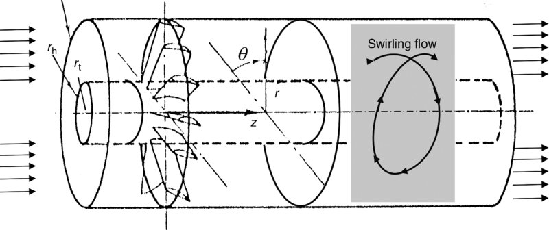
Turbomachinery is at the heart of gas turbine engines. The role of mechanical compression of air in an engine is given to the compressor. The shaft power to drive the compressor typically is produced by expanding gases in the turbine. The machines that exchange energy with a fluid, called the working fluid, through shaft rotation are known as turbomachinery. The machines where the fluid path is predominantly along the axis of the shaft rotation are called axial-flow turbomachinery. In contrast to these machines, in radial-flow turbomachinery the fluid path undergoes a 90° turn from the axial direction. These machines are sometimes referred to as centrifugal machines. A mixed-flow turbomachinery is a hybrid between the axial and the radial-flow machines. In aircraft gas turbine engines, the axial-flow compressors and turbines enjoy the widest application and development (Figure 8.1). The centrifugal compressors and radial-flow turbines are used in small gas turbine engines and automotive turbocharger applications.
FIGURE 8.1Schematic drawing of different types of compressors in aircraft gas turbine engines
8.2 The Geometry
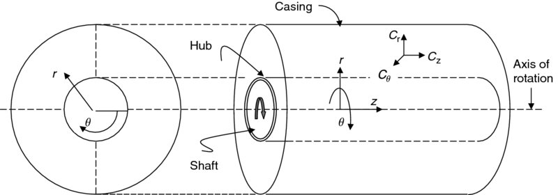
The geometry of rotating blades demands a cylindrical duct with a shaft centric configuration. This in turn leads to the choice of cylindrical coordinates for the analysis of flows in turbomachinery. The coordinates [r, θ, z] are in radial, tangential or azimuthal, and axial directions, respectively. The velocity components [Cr, Cθ, Cz] are the radial, tangential (or sometimes referred to as swirl or azimuthal velocity), and axial velocity components, respectively. These are shown in a definition sketch in Figure 8.2.
FIGURE 8.2Definition sketch for the coordinates and the velocity components of the flow in cylindrical coordinates
8.3 Rotor and Stator Frames of Reference
In turbomachinery, energy transfer between the blades and the fluid takes place in an inherently unsteady manner. This is achieved by a set of rotating blades, called the rotor. The rotor blades are three-dimensional aerodynamic surfaces, which experience aerodynamic forces. The rotor blades are cantilevered at the hub and thus feel a root bending moment and a torque. The reaction to the blade forces and moments is exerted on the fluid, via the action–reaction principle of Newton. Stationary blades called the stator follow the rotor blades in what is known as a turbomachinery stage. The stator blades are three-dimensional aerodynamic surfaces as well. They are cantilevered from the casing and experience forces and moments, like the rotor. The exception is that the stator forces and moments are stationary (in the laboratory frame of reference) and thus perform no work on the fluid. The energy of the fluid is, thus, expected to remain constant in passing through the stator blades. The position of the observer is, however, important in viewing the flowfield and the energy exchange in turbomachinery. An observer fixed at the casing (or laboratory) is called an absolute observer. If the observer is attached to the rotor blade and spins with it, then it is called a relative observer. The frames of reference are then called the absolute and relative frames of reference, respectively. Consider an isolated rotor in a cylindrical duct, as shown in Figure 8.3. An absolute observer sees the blades’ aerodynamic forces are in motion, at an angular rate, that is, the angular velocity w of the shaft. Hence, as measured by this observer, the total enthalpy of the fluid goes up in crossing the rotor row. On the contrary, let us put ourselves in the frame of reference of a relative observer who is spinning with the rotor. According to a relative observer, the blades are not moving! An observer fixed at the rotor measures aerodynamic forces and moments of the blades, however, as the forces are stationary, there is no work done on the fluid according to this observer. Thus, the relative observer measures the same total enthalpy across the blade row.
FIGURE 8.3Isolated rotor in a cylinder. Source: Adapted from Marble 1964
The flowfield as seen by a relative observer attached to an isolated rotor in a cylinder is thus steady. The absolute observer on the casing, however, sees the passing of the blades and thus experiences an unsteady flowfield. As the rotor blades pass by, a periodic pressure pulse (due to blade tip) is registered at the casing, which signifies an unsteady event with a periodicity of blade passing frequency. To be able to analyze a flowfield in a steady frame of reference offers tremendous advantages in the nature and the solution of governing equations. Consequently, in analyzing the flow within a rotor blade row, we employ the relative observer stance, while the stator flows are viewed from the standpoint of an absolute observer. We need to be mindful, however, that in practice there are no isolated rotors and thus the flowfield in rotating machinery is inherently unsteady. We shall present some preliminary discussions on the scale and effect of unsteadiness in axial-flow compressors later in this chapter.
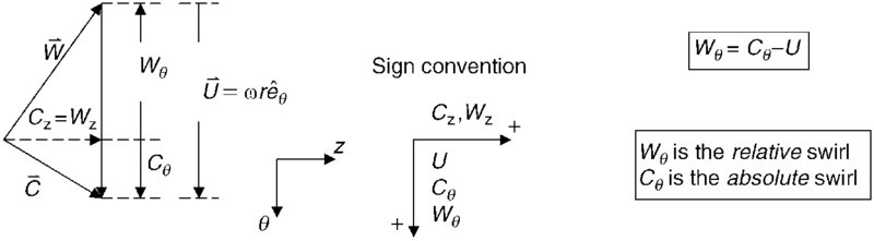
The velocity components as seen by observers in the two frames of reference are related. First, we note that the radial and axial velocity components are identical in the two frames, as the relative observer moves only in the θ, or the angular, direction. Therefore, the swirl or tangential velocity is the only component of the velocity vector field that is affected by the observer rotation. At a radial position r on the rotor, the relative observer rotates with a speed ωr and thus registers a tangential velocity, which is ωr less than the absolute swirl velocity, that is,
The fluid velocity vectors in the two frames are labeled as and for the absolute and relative observers, respectively. Therefore, the absolute velocity vector is described as
Comparing the velocity vectors as described by Equations 8.2–8.4, we conclude that the following vector identities hold, namely,
(8.5a)
(8.5b)
These three vectors form a triangle known as the velocity triangle.
Figure 8.4 shows a definition sketch of the velocity triangle and the sign convention. The positive tangential or azimuthal angle θ is in the direction of rotor rotation . The swirl velocity component is considered positive if in the direction of rotor rotation. For example, we note that the absolute swirl is pointing in the positive θ direction, therefore it is considered positive. The relative swirl velocity component Wθ is in the opposite direction, hence it is a negative quantity. The scalar relation given in Equation 8.1 between the two swirl components is always valid.
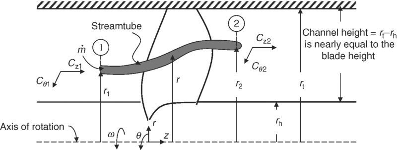
The Euler turbine equation is called the fundamental equation of turbomachinery. Once we derive this simple yet powerful expression, its significance becomes evident. Let us consider a streamtube that enters a turbomachinery blade row. Figure 8.5 illustrates a generic streamtube with its geometry and velocity components. In general, stream surfaces undergo a radial shift when interacting with a blade row, as depicted in Figure 8.5.
FIGURE 8.5Streamtube interacting with a turbomachinery blade row
The mass flow rate in the streamtube is constant, by definition, and is labeled as . The angular momentum of the fluid in the streamtube is the moment of the tangential momentum of the fluid about the axis of rotation, namely,
(8.6)
The change of fluid angular momentum between the exit and inlet of the streamtube is the applied torque exerted by the blade on the fluid, that is,
The torque is the product of blade tangential force Fθ and the moment arm r from the axis of rotation. Hence the blade torque is
(8.7b)
The expression 8.7a (or 8.7b) is valid for the rotor as well as the stator. In case of rotor, there is an angular motion, hence the product of the angular velocity of the blade and the torque provides the power transmitted to the fluid, namely,
(8.8)
The ratio of shaft power to mass flow rate is called the specific work of the rotor, wc for the compressor and wt for the turbine, hence,
This is the Euler turbine equation written for the fluid interacting with a compressor or turbine rotor. As evidenced in Equation 8.9, the rotor (specific) work appears as the change in (specific) angular momentum across a blade row times the shaft speed. The rotor and stator torques are proportional to the change in angular momentum across the rotor and stator blade rows, respectively, via Equation 8.7.
The first law of thermodynamics applied to a steady and adiabatic process demands that the change of total enthalpy of the fluid across the blade row to be equal to the blade-specific work delivered to the fluid, namely,
From the Euler turbine equation, the exit stagnation enthalpy in Equation 8.10a is related to the inlet stagnation enthalpy and the change of the angular momentum across the rotor row,
Note that we assumed a calorically perfect gas in Equation 8.10c when we replaced the ratio of stagnation enthalpy with the ratio of total temperatures.
8.5 Axial-Flow Versus Radial-Flow Machines
In an axial-flow turbomachinery, the fluid path is predominantly along the axis of rotation. In radial-flow or centrifugal machinery, the fluid path departs from axial and attains a predominantly radial motion at the exit. As a result, the following approximation is typically made for axial-flow machines,
(8.11)
Therefore, the Euler turbine equation may be simplified to
(8.12)
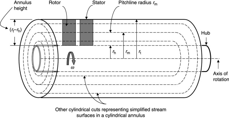
The assumption of constant “r” in axial-flow turbomachinery places the stream surfaces on cylindrical surfaces. This means that stream surfaces do not undergo significant radial deviation. Thus, radial deviation or radial shift of stream surfaces is often assumed negligible in axial-flow machines. The simplified flowfield in an axial turbomachinery annulus may be divided into a series of r = constant cylindrical cuts, as shown in Figure 8.6.
FIGURE 8.6A simple model of an axial compressor stage (rotor and stator) in a cylindrical annulus showing a mean or pitchline radius rm along with other cylindrical cuts of the annulus representing simplified stream surfaces
The pitchline radius rm is defined as the mid-radius between the hub and the casing, that is,
(8.13)
Often, the pitchline radius of an axial-flow turbomachinery is assumed to represent the mean or average of the flowfield properties in the annulus and thus serves as the first line of attack in a one-dimensional flow analysis approach. The hub and the tip radii represent the maximum deviations from the mean and thus are analyzed next. For a more accurate analysis, other cylindrical cuts are introduced in the annulus, as shown in Figure 8.6. To further improve the accuracy of our analysis, we need to incorporate the radial disposition of the stream surfaces interacting with turbomachinery blade rows. In general, the stream surfaces undergo a radial shift interacting with a blade row and thus form conical surfaces in the vicinity of a blade. We need to employ a three-dimensional flow theory such as radial equilibrium theory or an actuator disc theory to approximate their exit radius r2 of stream surfaces that have entered the blade row at the inlet radius of r1. We will estimate the radial shift of stream surfaces using radial equilibrium theory Section 8.6.5.
A centrifugal or radial compressor receives the fluid in the axial direction near the axis of rotation and imparts large angular momentum to the fluid by expelling the fluid at a higher radius and with a large swirl kinetic energy. The radial turbines receive the fluid at a large radius and with high swirl kinetic energy and expel the fluid near the axis of rotation with a small angular momentum. In the process of absorbing the swirl kinetic energy, a large blade torque is created, which in a rotor translates into shaft power. Hence, the radial shift of stream surfaces needs to be large for an efficient centrifugal compression/expansion and thus may not be neglected from our analysis. Fortunately, unlike axial-flow turbomachinery that we have to employ three-dimensional flow theories to predict the exit radius of an incoming stream surface, in a centrifugal machine the exit radius for all stream surfaces is fixed by the impeller geometry, that is, the impeller exit radius. We will treat centrifugal compressors in Chapter 9.
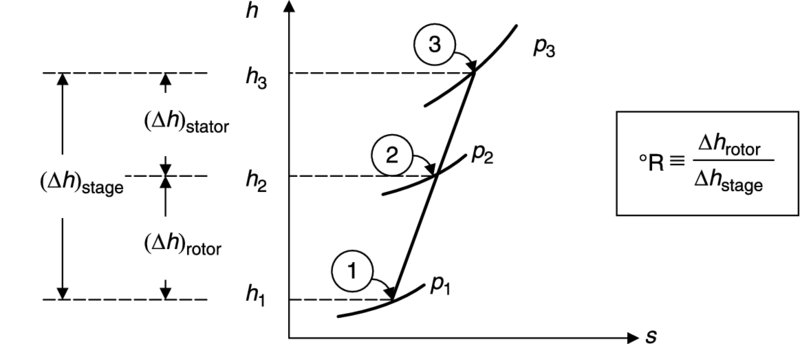
8.6 Axial-Flow Compressors and Fans
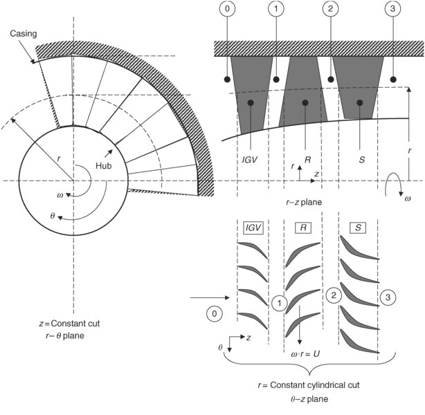
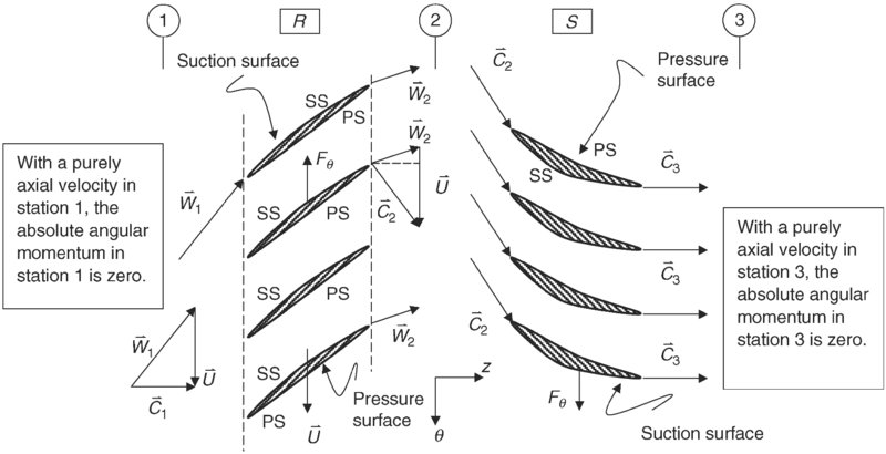
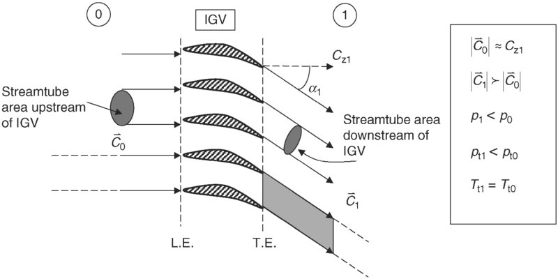
Axial-flow compressors and fans provide mechanical compression for the air stream that enters a gas turbine engine. Thermodynamically, their function is to increase the fluid pressure, efficiently. Hence, the boundary layers on the blades of compressors and fans, as well as their hub and casing, are exposed to an adverse, or rising, pressure gradient. Boundary layers exposed to an adverse pressure gradient, due to their inherently low momentum, cannot tolerate significant pressure rise. Consequently, to achieve a large pressure rise, axial-flow compressors and fans need to be staged. With this stipulation, a multistage machinery, or compression system, is born. In a stage, the rotor blade imparts angular momentum to the fluid, while the following stator blade row removes the angular momentum from the fluid. A definition sketch of a compressor stage with an inlet guide vane that imparts angular momentum to the incoming fluid is shown in Figure 8.7. A compressor stage without an inlet guide vane is depicted in Figure 8.8. In either case, the principle of rotor increasing the fluid angular momentum and the stator blade removing the swirl (or angular momentum) is independent of any preswirl in the incoming flow to the stage. We may introduce an inlet guide vane upstream of the rotor blades that imparts a preswirl (in the direction of the rotor motion) to the incoming stream and yet the principle of rotor–stator angular momentum interactions with the fluid remains intact.
FIGURE 8.7Definition sketch for station numbers and three different planes, r–θ, r–z, and θ–z, in a compressor stage with an inlet guide vane (IGV)
FIGURE 8.8Cylindrical (r = constant) cut of a compressor stage with velocity triangles showing the rotor imparting and the stator removing the swirl and angular momentum to the fluid
Based on the absolute velocity field in regions 1, 2, and 3, for a generic inlet condition that may include a preswirl Cθ1 created by an inlet guide vane, we may write the rotor and stator torques
(8.14)
(8.15)
Assuming the absolute swirl and angular momentum across the stage remains the same, that is, Cθ1 = Cθ3 and r1 = r3 the rotor and stator torques become equal and opposite, namely,
(8.16)
We observe the suction and pressure surfaces of the rotor and stator blades, as shown in Figure 8.8, and note that the blade aerodynamic forces in the θ-direction Fθ for the rotor and stator blades are in opposite directions. Since the moment of this tangential force, that is, r·Fθ from the axis of rotation, is the blade torque, we conclude that the rotor and stator torques are opposite in direction and nearly equal in magnitude.
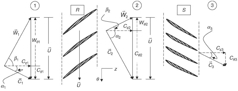
8.6.1 Definition of Flow Angles
The flow angles are measured with respect to the axial direction, or axis of the machine, and are labeled as α and β, which correspond to the absolute and relative flow velocity vectors and , respectively. Figure 8.9 is a definition sketch that shows the absolute and relative flow angles in a compressor stage.
FIGURE 8.9Definition sketch for the absolute and relative flow angles in a compressor stage (a cylindrical cut of the stage, r = constant)
We may use these absolute and relative flow angles to express the velocity components in the axial and the swirl direction as
One method of accounting for positive and negative swirl velocities is through a convention for positive and negative flow angles. We observe that the absolute velocity vector upstream of the rotor has a swirl component in the direction of the rotor rotation. Hence, the absolute flow angle α1 is considered positive. The opposite is true for the relative velocity vector , which has a swirl component in the opposite direction to the rotor rotation. Both the relative flow angle β1 and the swirl velocity facing it Wθ1 are thus negative.
A turbomachinery blade row is designed to maintain an attached boundary layer, under normal operating conditions. Hence, the flow angles at the exit of the blades are primarily fixed by the blade angle at the exit plane. For example, the relative velocity vector at the exit of the rotor, , should nearly be tangent to the rotor suction surface at the trailing edge. Hence, β2 is fixed by the geometry of the rotor and remains nearly constant over a wide operating range of the compressor. The same statement may be made about α1 or α3. These angles remain constant over a wide range of the operation of the compressor as well. Again, remember that the exit flow angle argument is made for an attached (boundary layer) flow. The other flow angles, as in β1 or α2, change with rotor speed U (i.e., ωr). Consequently, use is made of the nearly constant exit flow angles α1, β2, and α3 in expressing performance parameters of the compressor stage and the blade row.
The axial velocity components Cz1, Cz2, or Cz3 contribute to the mass flow rate through the machine. A common (textbook) design approach in axial-flow compressors and fans maintains a constant axial velocity throughout the stages. We shall make use of this simplifying design approach repeatedly in this chapter. Figure 8.8 shows an example of a constant axial velocity in a compressor stage. Although a simplifying design assumption, the reader needs to be aware that the goal of constant axial velocity is nearly impossible to achieve in practice. This is due to a highly three-dimensional nature of the flowfield, set up by three-dimensional pressure gradients, in a turbomachinery stage. We will address this and other topics related to three-dimensional flow in Section 8.6.5.
A useful concept in turbomachinery design calls for a repeated stage (also referred to as normal stage). This implies that the velocity vectors at the exit and entrance to a stage are the same, that is,
(8.21a)
(8.21b)
The velocity triangles at the inlet and the exit of the stage shown in Figure 8.8 have made use of the repeated stage concept. Another concept in turbomachinery calls for a repeated row design, which leads to flow angle implications that are noteworthy. In a repeated row design, the exit relative flow angle has the same magnitude as the absolute inlet flow angle, and the inlet relative flow angle has the same magnitude as the exit absolute flow angle, that is,
The example of the compressor stage shown in Figure 8.9 has used the concept of repeated row. Note that a repeated row design leads to a repeated stage but the reverse is not necessarily correct. Namely, we may have a repeated stage design that does not use a repeated row concept. Figure 8.8 shows an example of a repeated stage that does not obey a repeated row design.
8.6.2 Stage Parameters
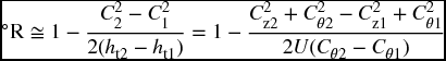
The Euler turbine equation that we derived earlier is the starting point for this section with the assumption of r1 ≈ r2 ≈ r,
We may replace the swirl velocities by the flow angles and the axial velocity components, namely,
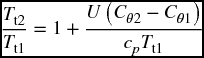
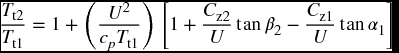
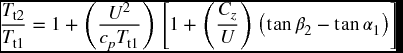
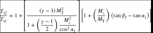
Expression 8.23 for the total temperature rise across the rotor (or stage) involves nondimensional groups Cz1/U and cpTt1/U2. These groups appear throughout the turbomachinery literature and deserve a special attention. Also, the axial velocity ratio Cz2/Cz1 appears that is often set equal to 1, as a first-order design assumption. Equation 8.23 is expressed in terms of the absolute flow angle at the exit of the rotor, which is not, however, a good choice, since it varies with the rotor speed. A better choice for the flow angle in plane 2, that is, downstream of the rotor, is the relative flow angle β2. The relative exit flow angle β2 remains nearly unchanged as long as the flow remains attached to the blades. To express the total temperature rise across the rotor to the flow angles α1 and β2, we replace the absolute swirl Cθ2 by the relative swirl speed, namely,
If we assume a constant axial velocity design, that is, Cz1 = Cz2, then we get
(8.25b)
Here, we have expressed the stage total temperature ratio as a function of two nondimensional parameters. Note that β2 is a negative angle and α1 is a positive angle, according to our sign convention. Therefore, the contribution to the stage total temperature ratio falls with increasing (Cz/U) for a given wheel speed and inlet stagnation enthalpy. The ratio of axial-to-wheel speed is called the flow coefficient
We may divide both numerator and the denominator of Equation 8.26a by the speed of sound in plane 1, that is, a1, to get the ratio of axial to blade (rotational) or tangential Mach number, namely,
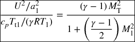
where Mz is the axial Mach number, and MT is the blade tangential Mach number based on U and a1. For example, a stream surface with an axial Mach number of 0.5 that approaches a section of a rotor that is spinning at Mach 1 has a flow coefficient of 0.5. Now, let us interpret the first nondimensional group U2/(cpTt1). We may divide this expression by the square of the upstream speed of sound to get
(8.27)
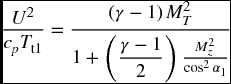
Noting that the absolute Mach number M1 is expressible in terms of the axial Mach number and a constant preswirl angle α1 as
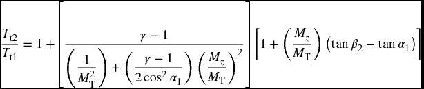
Kerrebrock (1992) offers an insightful discussion of compressor aerodynamics based on this equation. Two Mach numbers, that is, the axial and the blade tangential Mach numbers, appear to influence the stage temperature ratio in three ways, namely, via Mz, MT, and Mz/MT influence in Equation 8.30. However, if we divide the first bracket on the right-hand side (RHS) of Equation 8.30 by the square of the blade tangential Mach number, we reduce this dependency to two parameters, namely,
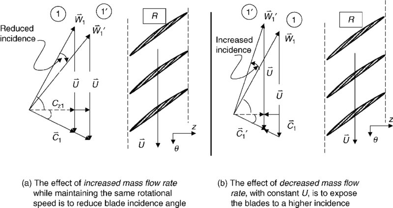
Consequently, two parameters govern the stage temperature ratio (or pressure ratio) and these are the blade tangential Mach number MT and the flow coefficient or the ratio of the axial-to-tangential Mach number Mz/MT. For given flow angles α1 and β2, an increase in the flow coefficient reduces the temperature rise in the stage. We may interpret an increase in the flow coefficient as an increase in the axial Mach number or the mass flow rate through the machine. As the mass flow rate increases, keeping the blade rotational Mach number the same, the blade angle of attack, or in the language of turbomachinery the incidence angle, decreases, hence the total temperature ratio drops. The opposite effect is observed with a decreasing mass flow rate through the machine where the incidence angle increases and thus blade work on the fluid increases to produce higher temperature or pressure rise. To visualize the effect of throughflow on rotor work, temperature and pressure rise, a rotor blade at different axial Mach numbers (or flow rate) and the same blade tangential Mach number (or wheel speed) are shown in Figure 8.10.
FIGURE 8.10Inlet velocity triangles for a compressor rotor with a changing flow rate
A reduced flow rate leads to an increased compressor temperature (or pressure) ratio. However, there is a limitation on how low the flow rate, or axial Mach number, can sink before the blades stall, for a fixed shaft rotational speed. Consequently, at reduced flow rates we could enter a blade stall flow instability, which marks the lower limit of the axial flow speed on the compressor map for a given shaft speed. The increased flow rate that leads to a reduction of the stage total temperature rise has its own limitation. The phenomenon of negative stall could be entered as the inlet Mach number is increased significantly.
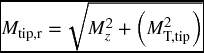
The second parameter is the blade tangential Mach number MT. A higher blade tangential Mach number increases the stage total temperature rise as deduced from Equation 8.31. However, the limitations on the blade tangential Mach number are the appearance of strong shock waves at the tip as well as the structural limitations under centrifugal and vibratory stresses. The rotor shock losses increase (nonlinearly) with the relative tip Mach number; however, the advantage of higher work (∝) on the fluid outweigh the negatives of such a design at modest tip Mach numbers. The relative tip Mach number is defined as
(8.32)
where it represents the case of zero preswirl. The general case that includes a nonzero preswirl, may be written as
(8.33)
The relative blade Mach numbers at the tip of operational fan blades have been supersonic for the past three decades. By necessity, these blade sections should be thin to avoid stronger bow shocks. A typical value for the relative tip Mach number is ∼1.2 but may be designed as high as ∼1.7. The thickness-to-chord ratio of supersonic blading may be as low as ∼3%. High strength-to-weight ratio titanium alloys represented the enabling technology that allowed the production of supersonic (tip) fans in the early 1970s.
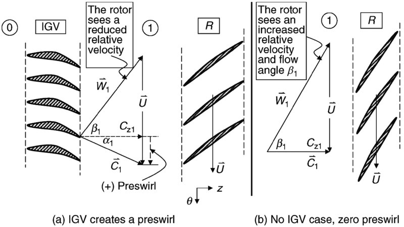
The inlet absolute flow angle to the rotor α1 is a design choice that has the effect of reducing the rotor relative tip speed. The inlet preswirl is created by a set of inlet guide vanes, known as an IGV. To reduce the relative flow to the rotor tip, the IGV turns the flow in the direction of the rotor rotation, by α1. The flowfield entering an IGV is swirl-free and thus the function of the IGV is to impart positive swirl (or positive angular momentum) to the incoming fluid. This in effect reduces the rotor blade loading whose purpose is to impart angular momentum to the incoming fluid. An inlet guide vane and its flowfield are shown in Figure 8.11.
FIGURE 8.11An inlet guide vane is seen to impart swirl to the fluid (note the shrinking stream tube area implies flow acceleration and static pressure drop)
We note that the blade passages in the IGV form a subsonic nozzle (i.e., contracting area) and cause flow acceleration across the blade row. The result of the flow acceleration is found in the static pressure drop due to flow acceleration, as well as a total pressure drop due to frictional losses of the blade passages. Hence, if the compressor design could avoid the use of an IGV, then certain advantages, including cost and weight savings, are gained. The advantage of operating at higher tip speeds at times outweighs the disadvantages of an IGV. The inlet guide vane may also be actuated rapidly if a quick response in thrust modulation is needed. For example, consider a lift fan, or a deflected engine exhaust flow, to support a VTOL aircraft in hover mode. The ability to modulate the jet lift (or vertical thrust) for stability and maneuver purposes may not be achieved through a spool up or spool down throttle sequence of the engine. Due to a large moment of inertia of the rotating parts in a turbomachinery, the rapid spooling is not fast enough for the control and stability purposes of a VTOL aircraft. In such applications, fast-acting IGV actuators could modulate the inlet flow to the rotor and hence the thrust/lift. An adjustable exit louver at the deflected nozzle end achieves the same goal. The inlet swirl angle α1 may be zero or be adjustable in the range of ±30° or more using a variable geometry IGV to relieve the relative tip Mach number, improve efficiency at compressor off-design operation, and provide for rapid thrust/lift modulation in military aircraft.
An example of a velocity triangle upstream of the rotor blade with and without the inlet guide vane is shown in Figure 8.12. In both cases, we maintain the rotational speed and the mass flow rate, i.e., the axial velocity Cz constant.
FIGURE 8.12Impact of IGV on the rotor relative flow for constant axial velocity and rotor speed
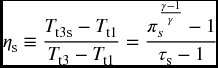
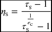
The stage total pressure ratio is related to the stage total temperature ratio via a stage efficiency parameter ηs. Recalling from the chapter on cycle analysis,
(8.34)
Therefore, we may calculate the stage total pressure ratio from the velocity triangles that are used in the Euler turbine equation to establish τs and an efficiency parameter ηs to get
(8.35)
Since the axial flow compressor pressure ratio per stage is small (i.e., near 1), the stage adiabatic efficiency and the polytropic efficiency are nearly equal. We recall that the polytropic efficiency was also called the “small-stage” efficiency, valid for an infinitesimal stage work. Although the approximation
(8.36)
is valid for low-pressure ratio axial flow compressor stages. The exact relationship between these parameters is derived in the cycle analysis chapter to be
(8.37)
Therefore, by calculating the stage total temperature ratio from the Euler turbine equation and assuming polytropic efficiency, of say 0.90, we may calculate the stage adiabatic efficiency. Otherwise, we may calculate the stage total pressure ratio from the polytropic efficiency ec and the stage total temperature ratio directly, via
(8.38)
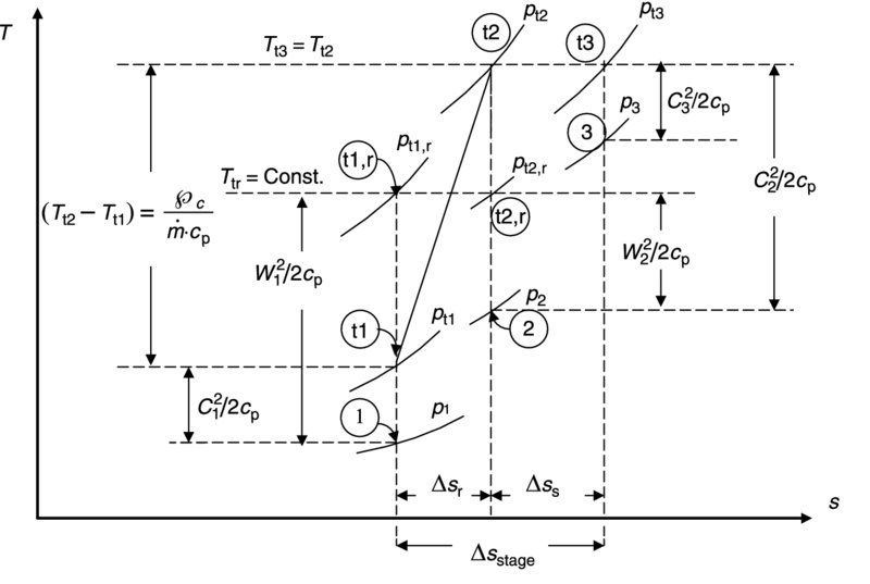
The frictional and shock losses are the main contributors to a total pressure loss in the relative frame of reference. We note that in a relative frame of reference, the blade passage is stationary and thus blade aerodynamic forces perform no work. Examining the fluid total pressure across the blade through the eyes of a relative observer, there are only losses to report. As noted, these losses stem from the viscous and turbulent dissipation of mechanical (kinetic) energy into heat as well as the flow losses associated with a shock. From the vantage point of an absolute observer, the blades are rotating and doing work on the fluid, thus increasing the fluid total temperature and pressure in the absolute frame of reference. These processes may be shown on a T–s diagram (Figure 8.13) that is instructive to review. For example, follow the static state of gas across the stage then follow the stagnation states in the absolute and relative frames. Explain the behavior of kinetic energy of gas as the fluid encounters the stationary and rotating blade rows, as seen by absolute and relative observers.
FIGURE 8.13Absolute and relative states of gas across a compressor rotor and stator
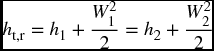
The relative total enthalpy is constant across the rotor along a stream surface (in steady flow without a radial shift in the stream surface),
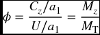
The function ψ is the nondimensional stage work parameter, which is called the stage-loading factor or parameter defined in Equation 8.44. The ratio of axial-to-wheel speed was called the flow coefficient , which forms another two-parameter family for the stage characteristics, namely,
We note that the rotor exit relative flow angle is a negative quantity that leads to a stage-loading factor that is less than 1. In the case of zero preswirl, or no inlet guide vane, the stage loading factor increases with a decreasing rotor exit flow angle β2. In the limit of zero relative swirl at the rotor exit and no inlet guide vane, the stage loading factor approaches unity. However, a rotor relative exit flow angle of zero implies significant turning in the rotor blade passage, which may lead to flow separation. The stage-loading factor is an alternate form of expressing the stage characteristics and, in essence, takes the place of the rotor tangential Mach number MT, which was presented earlier. Horlock (1973) takes advantage of the linear dependence of the stage loading and the flow coefficient in Equation 8.45 to explore the off-design behavior of ideal turbomachinery stages. We shall discuss the off-design behavior of turbomachinery later in this chapter but for now show the linear dependence of the two parameters in Figure 8.14 (adapted from Horlock, 1973).
FIGURE 8.14Linear dependence of stage loading and flow coefficient parameters in ideal turbomachinery stages. Source: Adapted from Horlock 1973
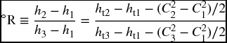
We define a stage degree of reaction °R as the fraction of static enthalpy rise across the stage that is accomplished by the rotor. Although the stator does no work on the fluid, it still acts as a diffuser that decelerates the fluid and thus causes an increase in fluid temperature, or static enthalpy. The stator takes out the swirl (kinetic energy) put in by the rotor and thus converts it to a static pressure rise. The degree of reaction measures the rotor share of the stage enthalpy rise as compared with the burden on the stator. This process is shown in an h–s diagram for the static states in a compressor stage. Remember that the static states are independent of the motion of the observer, hence they carry no subscript labels besides the station number (Figure 8.15).
(8.46a)
FIGURE 8.15Static states of gas in a compressor stage and a definition sketch for the stage degree of reaction °R
The stagnation enthalpy across the stator remains constant as the stator blades do no work on the fluid, hence ht3 = ht2 and if we assume a repeated stage, with C1 = C3, we simplify the above expression to get
(8.46b)
Now, for a constant axial velocity across the rotor, Cz2= Cz1, we get a simple expression for the stage degree of reaction, as
where Cθ, mean is the average swirl across the rotor. Since the flow has to fight an uphill battle with an adverse pressure gradient throughout a compressor stage, it stands to reason to expect/design an equal burden of the static pressure rise in the rotor as that of a stator. Consequently, a 50% degree of reaction stage may be thought of as desirable. We may express the swirl velocity components across the rotor in terms of the absolute in flow and relative exit flow angles, α1 and β2, respectively,
(8.47)
For a 50% degree of reaction stage (at some spanwise radius r), the rotor exit flow angle has to be equal in magnitude and opposite to the inlet absolute flow angle, which is dictated by an IGV, namely,
This is the condition for a repeated row design, as noted in Equations 8.22a and 8.22b. Therefore a purely axial inflow (with no inlet guide vane) demands a purely axial relative outflow in order to produce a 50% degree of reaction. Again, we need to examine the net turning angle across the blade and assess the potential for flow separation. We shall introduce another parameter that will shed light on the state of the boundary layer at the blade exit and that is the diffusion factor.
On the degree of reaction, there is a body of experimental results that support the proposal that a boundary layer on a spinning blade, that is, the rotor, is more stable than a corresponding boundary layer on a stationary blade, that is, the stator, hence allocating a slightly higher burden of static pressure rise to the rotor. Here the word stable is used in the context of resistant to adverse pressure gradient or higher stalling pressure rise. Based on this, a degree of reaction of 60% may be a desirable split between the two blade rows in a compressor stage. As we shall see in the three-dimensional flow section in this chapter, the desirable degree of reaction is often compromised at different radii along a blade span to satisfy other requirements, namely, a healthy state of boundary layer flow.
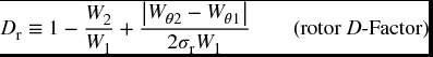
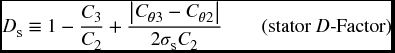
Another figure of merit for a compressor blade section that addresses the health of a boundary layer is, as noted earlier, the Diffusion Factor, or the D-factor. Its definitions for rotor and stator blades are, respectively
(8.48)
(8.49)
where σ defines the blade solidity, that is, the ratio of blade chord c to spacing s
(8.50)
(8.51)
Modern compressor design utilizes a high solidity (σm ≥ 1) blading at the pitchline radius (i.e., rm). Since the blade spacing increases linearly with radius, the solidity of a constant chord blade also decreases linearly with the blade span, that is,
where the Nb is the number of blades in the rotor or the stator row. We can see the variation of blade row solidity with blade span by substituting Equation 8.52 for the blade spacing, as
(8.53)
The hub section (rh) has thus the highest solidity and the tip section (rt) the lowest. The rationale for the definition of D-factor and its link to blade stall is made by Lieblein (1953, 1959, 1965). We review it here for its physical importance. First note that the definition of rotor diffusion factor is the same as the stator D-factor, except the parameters for the rotor are all in relative frame of reference. Next note that the change in swirl velocity across the rotor is the same regardless of the frame of reference, that is, the change in absolute swirl is the same in magnitude as the change in relative swirl, namely,
(8.54)
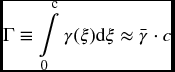
The blade circulation Γ is the integral of the vortex sheet strength γ over the chord, namely,
(8.55)
Figure 8.16 shows an element of a blade section represented by a vortex sheet of local strength γ(ξ). The local strength is equal to the local tangential velocity jump across the blade. The average vortex sheet strength is thus the average velocity jump across the sheet, namely,
(8.56)
FIGURE 8.16Blade airfoil section is represented by a vortex sheet and a velocity distribution
Therefore, the average (positive) circulation around the blade section is
(8.57)
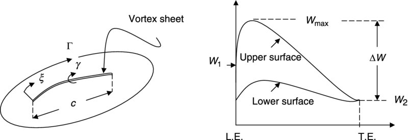
Now, let us consider a control volume symmetrically wrapped around a blade section, as shown in Figure 8.17.
FIGURE 8.17Control volume for determining the blade circulation Γ along a stream surface
By performing a closed line integral in the clockwise direction around the path C (Figure 8.18), we calculate the magnitude of blade circulation Γ as
Therefore equating the two expressions for the (magnitude of) blade circulation, we get
(8.59)
The maximum adverse pressure gradient on the blade suction surface leads to a maximum flow diffusion, which may be measured by the following parameter
(8.60)
This parameter is called the Diffusion Factor D
(8.61)
8.6.3 Cascade Aerodynamics
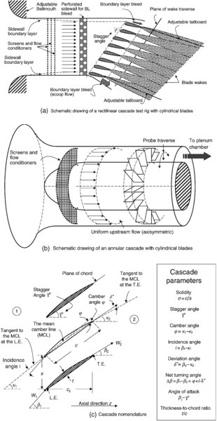
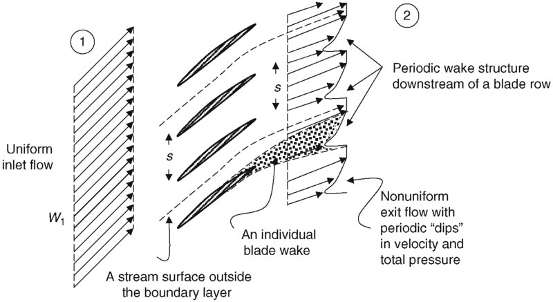
A large body of experimental data supports a correlation between the blade stall and the diffusion factor. Let us first examine the attributes of a stalled flow in a compressor blade row. A separated boundary layer will create a thick wake, which may be characterized by its momentum deficit length scale θ*. Equivalently, a wake is a region of deficit total pressure, hence in the blade frame of reference stall creates a rapid rise in the total pressure loss across the blade row. In either case, we need to examine the wake profile downstream of a blade row to quantify momentum and total pressure loss. To concentrate on the study of compressor blades, NACA (the predecessor of NASA) developed the so-called 65 series of airfoil profiles in early 1950s. To test the aerodynamic behavior of the newly developed blade shapes, NACA performed an extensive series of cascade experiments, concentrating on the impact of the 65-series compressor airfoil shapes on two-dimensional compressor loss and stall characteristics. Airfoil shapes are defined around a mean camber line, typically of circular arc or parabolic shape and a prescribed thickness distribution. A cascade is composed of a series of two-dimensional or cylindrical blades placed in a uniform flow to simulate the two-dimensional flowfield about a spanwise section of a compressor blade row. The goal of the investigation is to quantify the profile loss of two-dimensional blade elements as a function of the profile geometry and cascade parameters such as blade chord-to-spacing ratio, blade stagger angle, and other parameters. To construct the three-dimensional loss characteristics of compressor blades, two-dimensional cascade loss data are stacked up to represent the 3D picture. This approach neglects the cross interaction of the stream surfaces that is created through 3D pressure gradients. We learned in wing theory that three-dimensional pressure gradients lead to the formation of the streamwise vortices in the wake, which causes a 3D induced velocity (and induced drag) along the blade span. We shall address three-dimensional losses that are overlooked by the cascade data later in this chapter. Let us return to two-dimensional cascade studies performed at NACA. The wake profile with its momentum deficit and total pressure loss holds the key to characterizing the behavior of a compressor blade section. Figure 8.18a shows a rectilinear cascade, Figure 8.18b an annular cascade, and Figure 8.18c defines the geometric parameters of the blade section and the cascade. Figure 8.19 shows periodic blade wakes downstream of a cascade where the momentum deficit and the total pressure loss are concentrated. The thickness of the wake is exaggerated in Figure 8.19 for visualization purposes, but a thicker suction surface boundary layer than the pressure surface is intentionally graphed to show the behavior of these boundary layers that merge to form the blade wake in turbomachinery.
FIGURE 8.19Survey of the wake-velocity profile downstream of a cascade
Let us review the cascade parameters as shown in Figure 8.18c. An important geometrical cascade parameter is the solidity σ, which is defined as the ratio of chord-to-spacing. A high solidity blading is capable of a higher net turning angle than a low solidity blading. Consequently, a high solidity cascade is less susceptible to stall. Experimental evidence to support this assertion will be presented as cascade test results. As noted earlier, the modern compressor and fan design utilizes a high solidity blading (σt ≅ 1). The angle of the mean camber line at the leading and trailing edge is used as a reference where we measure the inlet flow incidence angle i and the exit deviation angle δ*. The incidence angle is defined as the flow angle between the tangent to the mean camber line and relative velocity vector at the inlet. In compressors, incidence angle takes the place of angle of attack in external aerodynamics. An optimum, incidence angle is defined as the incidence that causes minimum (total pressure) loss across a given cascade. A typical value of the optimum incidence angle for a subsonic flow cascade is iopt ∼ 2°. Cascade experimental results support this rule of thumb. The camber angle ϕ is defined as the angle formed at the intersection of the two tangents to the mean camber line at the leading and trailing edges, as shown. A large camber means a large flow turning, which may lead to flow separation. Hence, compressor blade camber is small compared with a turbine blade, which is capable of large turning due to a favorable pressure gradient. The stagger angle γ° is sometimes referred to as the blade-setting angle is the blade chord angle with respect to the axial direction. The stagger angle increases with radius as the blade rotational speed (ωr) increases linearly with radius. The difference between the stagger angle and the relative inflow angle is called the angle of attack, as in external aerodynamics. Finally, the net turning angle refers to the difference between the inlet and exit flow angles, respectively.
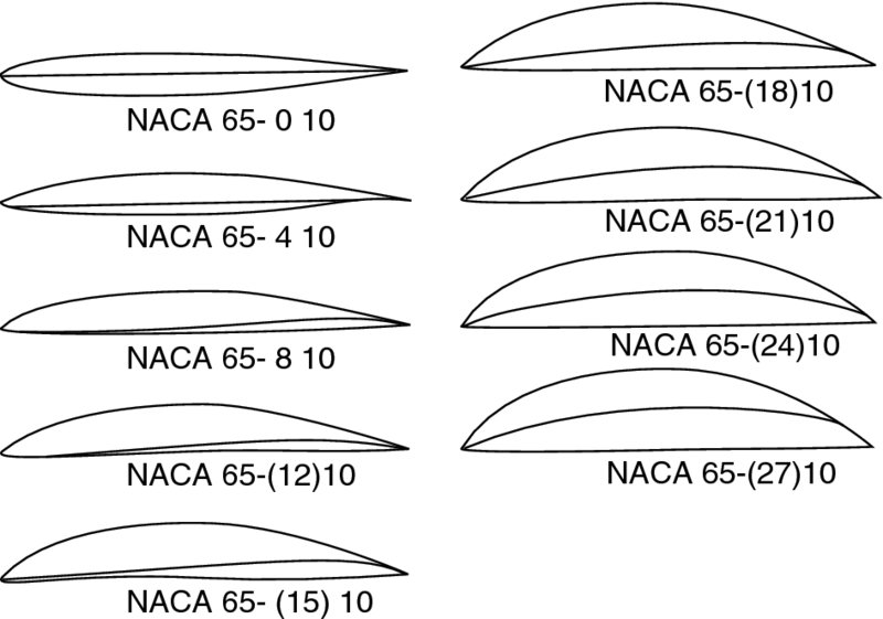
The 65-series compressor cascade airfoil shapes are shown in Figure 8.20. The design (theoretical) lift coefficient for an isolated airfoil shape (at zero angle of attack) is listed in parenthesis (times ten) following the 65-series designation. Note that the lift coefficient at zero angle of attack is entirely due to camber. The isolated means that the airfoil is not in a cascade configuration, that is, solidity is zero. The thickness-to-chord ratio (in percent) comprises the last two digits of the series designation.
FIGURE 8.20The 65-series cascade airfoil shapes with 10% thickness. Source: Herrig, Emery, and Erwin 1951
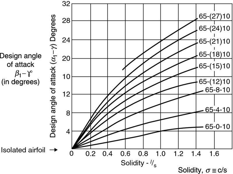
For example, a NACA 65-(18)10 represents the 65-series camber shape that produces an isolated theoretical (i.e., inviscid) lift coefficient of 1.8 (at zero angle of attack) and has a 10% thickness-to-chord ratio. The cascade parameters, namely, solidity and stagger, are included in the individual loss characteristic (bucket) curves that are produced for different cascades. NACA defined a design angle of attack for the 65-series airfoils based on the smoothness of the pressure distributions on the airfoils. Figure 8.21 shows the design angle of attack for the 65-series airfoils arranged in a cascade of varying solidity. The zero solidity refers to an isolated airfoil case. Note that the combination of high solidity and high camber that leads to a high angle of attack (Figure 8.21) does not mean that the incidence angle is very large too. The blade inlet angle κ1 makes a large angle with respect to the blade chord for highly cambered airfoils (see Figure 8.20 for airfoil shapes with high camber). The message from Figure 8.21 is that higher solidity allows for larger turning, which translates into an increase in inlet flow angle (keeping the exit angle ∼ fixed).
FIGURE 8.21Design angle of attack, β1– γ°, for the 65-series airfoils with 10% thickness as a function of solidity. Source: Herrig, Emery, and Erwin 1951
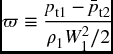
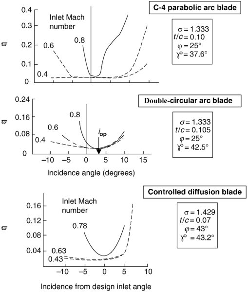
A survey of total pressure downstream of cascade reveals the presence of periodic wakes. Defining an average total pressure loss parameter for a cascade as
where the average downstream total pressure may be taken as the area-average of the total pressure survey. The denominator of Equation 8.62 is the familiar dynamic pressure (ρ1/2) in the cascade frame of reference. The cascade loss “bucket curves” are shown in Figure 8.22 for a parabolic arc, a double-circular arc, and a controlled diffusion blading at different inlet Mach numbers (adapted from Kerrebrock, 1992). The works of Hobbs and Weingold (1984) and Hechert, Steinert and Lehmann (1985) on development of controlled diffusion airfoils and their comparison to NACA-65 airfoils for compressors should be consulted for further reading.
FIGURE 8.22Variation of cascade total pressure loss parameter with inlet Mach number and flow incidence angle. Source: Adapted from Kerrebroch 1992
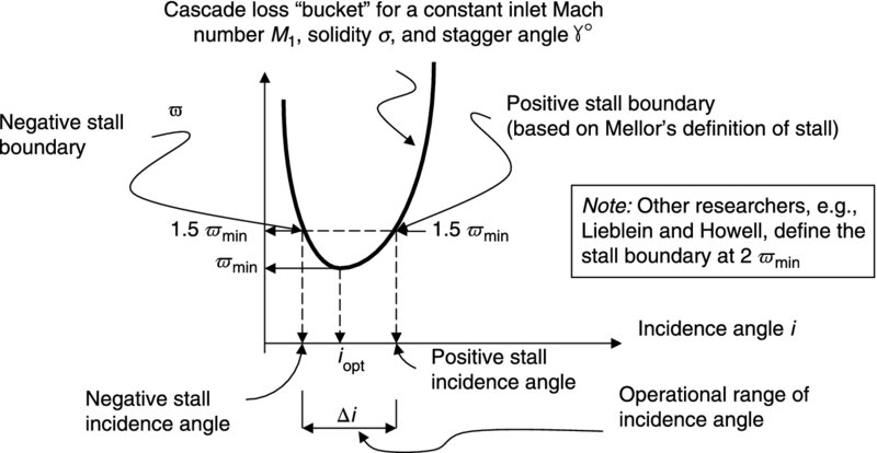
The minimum loss incidence angle is referred to as ϖmin that corresponds to the optimum incidence angle iopt We further define an acceptable operational range for the incidence angle that corresponds to 150% of the minimum loss ϖmin, which Mellor referred to as the positive and negative stall boundaries. A definition sketch is shown in Figure 8.23.
FIGURE 8.23Definition sketch for the stall boundaries based on the cascade loss curve
Mellor presents the operational range of each 65-series airfoils in various cascade arrangements that are very useful for preliminary design purposes. Mellor’s unpublished graphical correlations (originated at MIT Gas Turbine Laboratory) were published by Horlock (1973), Hill and Peterson (1992), among others.
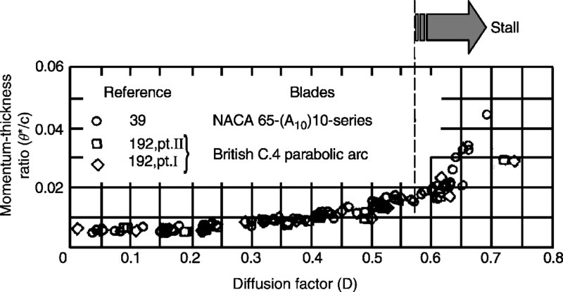
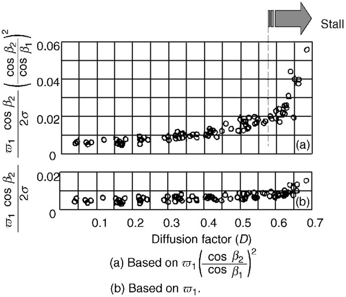
The correlation between the diffusion factor and the wake momentum deficit thickness θ* is presented in Figure 8.24 (Lieblein, 1965). The cascade data of Lieblein present 10% thick blades with the mean camber line shapes described by the NACA 65-series profiles and the British C-4 parabolic arc profiles, as shown in Figure 8.24. The Reynolds number for the cascade tests is ∼250, 000. Blade stall leads to a thickening of the wake that results in a rapid increase in profile drag and hence momentum deficit thickness. From Figure 8.24, we note this behavior occurs around a D-factor of 0.6. Hence, the maximum diffusion factor associated with a well-behaved boundary layer on these classical blade profiles is Dmax ∼ 0.6. A higher D-factor (of ∼0.7) may be achieved in cascades of modern controlled-diffusion profiles.
FIGURE 8.24Correlation between the diffusion factor and the wake momentum deficit thickness. Source: Lieblein 1965 (reference numbers are in Lieblein). Courtesy of NASA
How does the momentum deficit thickness θ*/c relate to the total pressure loss parameter ϖ in a cascade? By averaging the total pressure downstream of the cascade assuming a periodic momentum deficit thickness with zero momentum, we can correlate these two parameters. Figure 8.25 (Lieblein, 1965) shows two total pressure loss functions and their correlation with D-factor.
FIGURE 8.25Total pressure loss correlation with D-factor. Source: Lieblein 1965. Courtesy of NASA
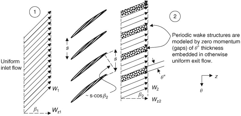
To demonstrate the functional form of the correlation (see the ordinate of Figure 8.25), we approximate the cascade exit flow as being composed of uniform flow with periodic gaps of zero momentum, each with θ*/c thickness corresponding to wakes. The static pressure is assumed to be uniform in the measuring station downstream of the cascade. Figure 8.26 shows a definition sketch of this simplified cascade exit flow model. Although the original contribution to this derivation is due to Lieblien-Roudebush (1956), this author has benefited from Kerrebrock’s (1992) treatment of this and other turbomachinery subjects.
FIGURE 8.26Definition sketch for a cascade exit flow model with periodic wakes
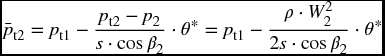
The total pressure downstream of the cascade is the sum of static and dynamic pressures, according to (incompressible) Bernoulli equation. The dynamic pressure is zero in the wake region of θ* thickness. We may area-average the total pressure in the downstream region according to
(8.63a)
(8.63b)
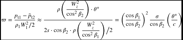
Note that we have used the concept of constant total pressure in an inviscid fluid by using pt1 = pt2 outside the wake region. Therefore, in the blade frame of reference, the total pressure remains conserved in the inviscid limit, assuming there are no shocks in the blade passage. In this context, we have applied the Bernoulli equation, which strictly speaking holds for an incompressible fluid. All these approximations are reasonable for our purposes here of demonstrating subsonic cascade data correlation of total pressure loss with D-factor. Now, in terms of the total pressure loss parameter ϖ we get
(8.64)
Here we made a simple approximation of constant axial flow across the cascade. Finally, we conclude that since θ*/c correlated with the diffusion factor, then the RHS of
(8.65)
correlates with the D-factor as well, keeping other cascade parameters constant. This functional dependence of the total pressure loss parameter on D-factor is demonstrated in Figure 8.25.
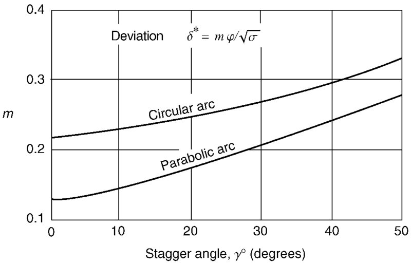
The exit flow angle deviates from the exit blade angle by what is called a deviation angle δ* due to boundary layer buildup at the trailing edge. Cascade experiments have revealed a correlation between the deviation angle and the geometric parameters of a cascade, namely, the camber angle, the solidity, and the stagger angle. The following correlation is due to Carter (1955).
(8.66)
where ϕ is the camber angle, σ is the solidity, m is a function of cascade stagger angle, and n is 1/2 for a compressor cascade and 1 for an inlet guide vane (or an accelerating passage such as turbines). The higher exponent of solidity for a turbine (n = 1) than the compressor (n = 1/2) leads to higher exit deviation angles in a compressor, as expected. The boundary layer build up in a compressor in adverse pressure gradient is greater than its counterpart in the turbine. The dependence of m on stagger angle and the profile shape is presented in Figure 8.27, following Carter (1955).
FIGURE 8.27Compressor cascade deviation angle rule following Carter (1955). Source: Reproduced with permission from Elsevier
The double-circular arc blade has a circular arc mean camber line shape where the point of maximum camber and thickness occur at mid-chord. The parabolic arc mean camber line blade that is shown in Figure 8.27 has a maximum camber location at 40% chord. The location of the maximum camber and even the thickness affect the pressure distribution about the blade and hence the exit flow deviation angle. It is instructive to know that in turbomachinery blading the chordwise location of the maximum camber moves farther aft with an increasing inlet relative Mach number. For example, a multiple-circular arc blade may be used in the supersonic section of a transonic compressor with the maximum camber placed at 75% chord. We shall discuss multiple-circular arc and other profile shapes of suitable blades for supersonic applications later in this chapter.
A more general definition of the diffusion factor should involve the radial shift of stream surfaces across compressor blade rows. The constant radius, cylindrical cut approximation of the flowfield is rather restrictive. The method allows for a “pitchline, ” one-dimensional analysis of a compressor, but falls short of a realistic “mean” flow modeling. A general D-factor is defined as
(8.67)
Note that the change in angular momentum has replaced the change in tangential momentum in the definition of a general D-factor. We will address the general diffusion factor in the three-dimensional flow section in this chapter.
Another performance limiting parameter in a compressor in addition to the D-factor is the static pressure rise coefficient, as in a diffuser. The pressure rise coefficient and the D-factor are two different ways of measuring the same thing, namely, the tendency of the boundary layer to stall. However, the D-factor examines the stall behavior of a compressor blade suction surface, whereas the stalling pressure rise coefficient analogy with a diffuser examines the end wall stall that dominates the multistage compressor aerodynamics. The new limiting parameter is defined as
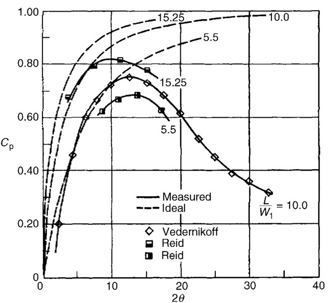
The static pressure rise across a blade row, in the numerator of Equation 8.68, is independent of the observer frame of reference. The dynamic pressure at the inlet to the blade row is in the relative frame, that is, as in a cascade parameter. From our studies of boundary layers in adverse pressure gradient we have learned that Cp, max ≈ 0.6. Interestingly, the numerical values of Cp, max and the limiting D-factor are both ∼0.6, a coincidence. The nature of the compressor end wall boundary layer and its stalling characteristics is more complicated than a simple diffuser. Figure 8.28 shows the pressure rise data for a two-dimensional diffuser, where a working range of Cp within ∼0.4 to ∼0.8 is observed (from Kline et al., 1959).
FIGURE 8.28Static pressure rise limitation in a 2D diffuser (data from Kline, Abbott and Fox 1959). Source: Kline, Abbott and Fox 1959. Fig. 4, p. 326. Reproduced with permission from ASME
The main differences between a diffuser flow and a flow in a compressor blade row are
Compressor boundary layer is highly skewed due to large streamwise and radial pressure gradients, that is, leading to (a highly) three-dimensional flow separation
Inherent unsteadiness in turbomachinery due to relative motion of neighboring blade rows are absent in a diffuser
Compressibility effects through the passage shock interaction with the boundary layer is absent in diffuser performance charts such as Figure 8.28
Upstream wake transport in downstream blade rows is also absent in diffusers
Blade tip clearance flow is unique to turbomachinery
End wall regions create secondary vortex formations as in corner and scraping vortex structures in compressors with no counterpart in a diffuser
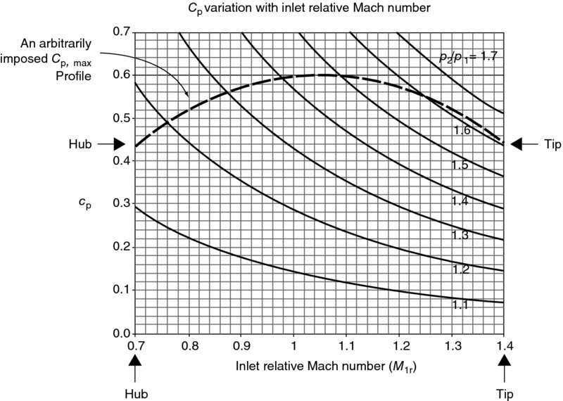
In light of these complicating factors, to suggest a single value for the maximum (sometimes called stalling) pressure rise coefficient for all compressor blade sections is oversimplistic. For example, the stalling pressure rise coefficient near the end walls may be ∼0.48 (first stipulated by de Haller, 1953) and at the pitchline radius ∼0.6. A stalling pressure rise correlation for multistage axial-flow compressors is successfully derived by Koch (1981). We will present Koch’s correlation in the context of compressor stall margin later in this chapter. A simple application of de Haller pressure rise criterion in the incompressible limit restricts the maximum flow deceleration (W2/W1) in a blade row to 0.72. The shock in passage also changes the abruptness of the static pressure rise, hence the boundary layer separation. Despite these shortcomings, the concept of a stalling pressure rise in a compressor blade row is very attractive and useful. We shall examine some limiting features of stalling pressure rise coefficient in a compressor blade. First, let us use Bernoulli equation in recasting the static pressure rise coefficient Cp as
The cascade total pressure loss parameter ϖmin is ∼2% for unstalled blades (Figure 8.21). For a maximum pressure rise coefficient of ∼0.6, the maximum flow deceleration (expressed in terms of W2/W1) is
The implication of this (maximum) flow deceleration may be found in the turning angle limitation, namely, for a constant axial velocity Wz, we have W1 = Wz/cosβ1 and W2 = Wz/cosβ2,
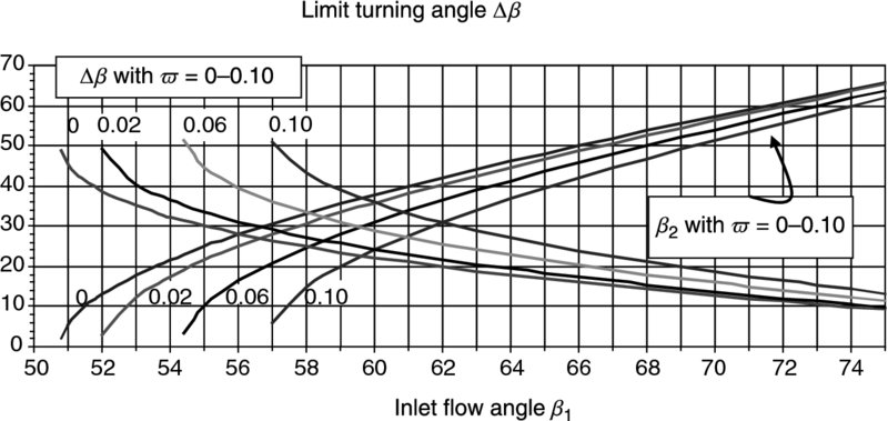
We may solve Equation 8.20 for the exit flow angle β2 for a given cascade total pressure loss parameter, inlet flow angle, and the maximum pressure rise coefficient. The maximum turning angle (Δβ) associated with a limiting pressure rise coefficient is graphed in Figure 8.29. The cases of zero total pressure loss, that is, ideal flow, and a cascade with a total pressure loss parameter of 2, 6, and 10% are shown. The effect of total pressure loss increase is seen in Figure 8.29 as a reduction in exit flow angle and thus an increase in flow turning in a compressor blade row. Also, from Equation 8.70, we observe that the maximum static pressure rise coefficient Cp, max for a given inlet flow angle β1 and total pressure loss occurs at the exit flow angle β2 = 0, or axial flow direction at the exit, as expected.
FIGURE 8.29The exit flow and the limit turning angles (in degrees) based on a Cp, max of 0.6
Another aspect of the pressure rise coefficient may be found in its relation to the relative inlet Mach number M1r. From the definition of the static pressure rise coefficient, we may express the dynamic pressure in terms of the inlet static pressure and the inlet relative Mach number, as
(8.71a)
(8.71b)
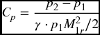
In a modern transonic fan or compressor stage, the relative Mach number to the rotor varies from hub-to-tip of ∼0.7 to ∼1.4, respectively. The variation of feasible static pressure ratio along the blade span with relative Mach number is shown in Figure 8.30.
FIGURE 8.30Variation of static pressure rise coefficient Cp with inlet relative Mach number (for constant pressure ratio p2/p1) with an arbitrarily imposed Cp, max profile
We observe that the static pressure ratio p2/p1 is nearly limited by ∼1.15 near the hub and may increase to ∼1.6 for a supersonic relative tip Mach number for a Cp, max of ∼0.45 near the tip. The static pressure distribution downstream of a turbomachinery blade row strongly depends on the swirl distribution and the axial velocity profile in the spanwise direction. The most common approach in preliminary analysis of three-dimensional flows in turbomachinery is the radial equilibrium theory that we shall discuss in this chapter.
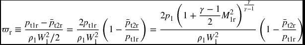
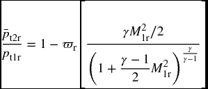
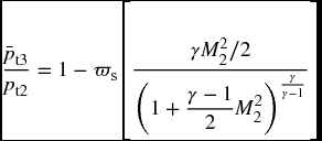
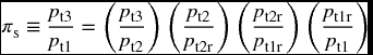
It is useful to correlate the compressor stage efficiency, at a given radius, with the cascade loss coefficients at the corresponding radius. Let us consider the cascade total pressure loss coefficients of ϖr and ϖs to represent the relative total pressure loss in the rotor and the stator blade sections, respectively, nondimensionalized with respect to the inlet dynamic pressure.
(8.72)
We may also express the ratio of static pressure to dynamic pressure in terms of the relative Mach number to simplify the above expression as
Equations 8.73 and 8.74 describe two of the parentheses in Equation 8.76, and we may relate the remaining two expressions to flow Mach numbers in the absolute and relative frame, namely
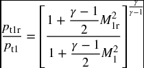
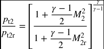
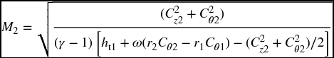
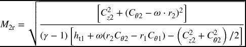
From the inlet conditions, we can calculate M1 and M1r that are needed in Equation 8.77. The absolute and relative Mach numbers in station 2, that is, downstream of the rotor, may be calculated from the velocities C2 and W2 from the velocity triangles and the speed of sound a2. The speed of sound may be related to fluid total enthalpy and kinetic energy according to
(8.79)
Therefore,
(8.80)
Hence, the absolute Mach number downstream of the rotor, in terms of known quantities, is
(8.81)
The relative Mach number M2r is
(8.82)
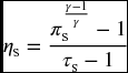
Now, we have established all the parameters that enter the stage adiabatic efficiency Equation 8.75 in terms of the basic velocity triangles and the cascade total pressure loss coefficients. Our analysis is valid for compressible flows in turbomachinery. However, by limiting the analysis to incompressible fluids, we may relate the stage efficiency to the stagnation pressure loss in the rotor and stator blade rows, via
The derivation of Equation 8.83 is straightforward and is shown in Hill and Peterson (1992). The cascade total pressure loss data directly feed into Equation 8.83 for the stage efficiency estimation. In general, we have to supplement the cascade total pressure loss coefficient by shock losses in supersonic flow. In addition, we need to account for the effect of the shock-boundary layer interaction, which increases the blade profile losses. These effects belong to what is known as the compressibility effects. A host of other losses in a turbomachinery stage occur that are not usually simulated in a cascade experiment. For example, the end-wall effects, including the tip clearance flow, the streamwise vortices in the blades’ wakes due to spanwise variation of blade circulation, as well as flow unsteadiness that result in vortex shedding in the wakes, are not simulated in a typical cascade experiment. The cascade total pressure loss parameter ϖ describes the profile loss of a two-dimensional blade in a steady flow. We will use it as a foundation to construct a more elaborate blade loss model, only.

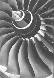
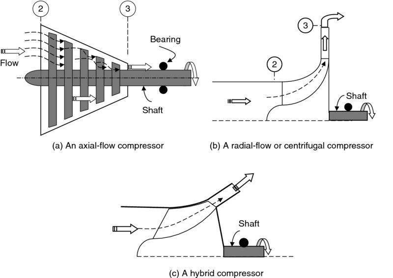
 FIGURE 8.1 Schematic drawing of different types of compressors in aircraft gas turbine engines