
10.2.4.2 Impingement Cooling
The turbine blade stagnation point, near the leading edge, represents the highest heat flux area of the blade. A typical heat flux distribution on a turbine blade (for a given free-stream turbulence intensity) is presented in Figure 10.41. “s” is a natural coordinate measuring the surface length from the leading edge on the suction and pressure surfaces. Due to longer length of the suction surface, as compared with the pressure surface, and a different location of the transition point on the two sides of the blade, the heat flux graph looks lob-sided.
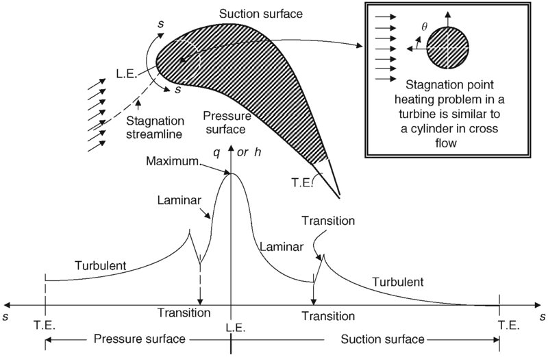
 FIGURE 10.41 Schematic drawing of heat flux q (or heat transfer coefficient h) distribution on an uncooled turbine blade (for a free-stream turbulence intensity)
An important observation (from Figure 10.41) is that the highest heat flux occurs at the leading edge, or the stagnation point heating in a turbine blade is the most critical. The second message is the rapid rise of heat transfer due to boundary layer transition from laminar to turbulent. The third observation is the curvature switch from convex to concave on the suction and pressure surfaces, respectively, thus affecting the transition point on the blade. In the theory of curved viscous flows, a convex curvature has a stabilizing effect on the flow, whereas a concave curvature has a destabilizing effect. The concave curvature case leads to the appearance of streamwise Goertler vortices that cause an enhanced mixing of the flow at the surface. The free-stream turbulence intensity Tu also enhances the heat transfer to a surface in two ways; (1) it promotes earlier transition and (2) it enhances mixing at the surface. An accepted correlation for leading-edge heat transfer finds its roots in a cylinder in cross flow problem (Colladay, 1975), which is
where
- a augmentation factor (from 1.2 to 1.8, based on free-stream turbulence)
- D diameter of leading-edge circle
- Φ angular distance from the leading-edge stagnation point, in degrees
To effectively cool the leading edge of a turbine blade, the internal cooling passage at the nose “showers” the leading edge with the coolant through a series of holes, as shown in Figure 10.42. Since the angle of impact between the coolant and the surface is nearly normal, the name “impingement” is attributed to this type of cooling. Some of the coolant that enters the leading-edge channel may discharge through the blade tip or it may be confined to within the blade. The example shown in Figure 10.42b has sealed off the nose channel exit, thus the entire coolant is used in the impingement cooling of the blade leading edge. To study heat transfer correlations with impingement cooling, Kercher and Tabakoff (1970) may be consulted.

FIGURE 10.42 Schematic drawing of an impingement cooling scheme suitable for the leading edge of a turbine blade
10.2.4.3 Film Cooling
The most critical areas of a turbine blade may be film cooled through a row of film-cooling holes. The coolant is ejected through a hole at an angle with respect to the flow, which in turn bend and cover a portion of the surface with a “blanket” of coolant.
Figure 10.43a shows a slanted jet emerging from a surface at an angle. Note the scale of the gas boundary layer thickness δ as depicted in Figure 10.43a, and compare it to the penetration of the coolant jet in the hot gas flow. The coolant jet penetrates the hot gas free stream (i.e., inviscid core) and is deflected by the external forces in the free stream. The penetration of the slanted film columns in the free stream and the associated local flow separation immediately downstream of the film hole causes the profile drag of turbine blades to increase. Therefore, the film cooling of turbine blades is more disruptive to the external aerodynamics of the blades, as compared with internal cooling scheme. The contours of constant heat flux are shown in Figure 10.43b.

FIGURE 10.43 Coolant ejection from a film hole on a turbine blade
The cooling effect of the ejected jet that emerges from the film hole covers only a small region in the immediate vicinity of the ejection hole. For this reason, practical film cooling in gas turbines involves numerous film holes in one or multiple (staggered) rows to cover a significant portion of a surface. Figure 10.45 shows a staggered array of two rows of film holes with typical length scales, that is, hole diameter D and spacing (or pitch P) that are noted on the graph.

FIGURE 10.44 Schematic drawing of a film-cooled turbine blade (with six film holes)
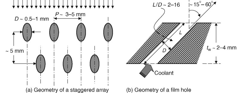
FIGURE 10.45 Definition sketch used in film cooling and some typical scales
The diameter of the film holes range ∼ 0.5 − 1 mm. Although it is possible to reduce the film-hole diameter to below 0.5 mm using advanced manufacturing techniques (e.g., using electron beam), in practice such small holes are prone to clogging, especially in the gas turbine environment. The products of combustion include particulates and by-products that cling to surface and clog the film holes. It is intuitively expected that the nondimensional pitch-to-diameter ratio of the film hole P/D to be an important parameter in heat transfer, thus film-cooling effectiveness. Also, the length-to-diameter ratio L/D for the film hole is important in the lateral spread of the film, and the size of the local separation bubble immediately downstream of the film hole. To add to the complexity of the film cooling, we note that the shape of the coolant plenum chamber also impacts the coolant jet velocity distribution and its mixing with the free stream and thus important to the film-cooling effectiveness. A specialized reference on the fundamentals of film cooling and gas turbine heat transfer is the von Karman Lecture Series (VKI-LS 1982).
A film-cooling effectiveness parameter ηf may be defined as

where the only new temperature in the equation, that is, Taw-f, is the adiabatic wall temperature in the presence of the film and excluding other cooling effects. Note that the true adiabatic wall temperature with film cooling, Taw-f, is a very difficult parameter to measure. Therefore, it is possible (and preferable) to define a film-cooling effectiveness parameter that utilizes a different and more easily measured temperature in the experiment, for example, the actual wall temperature, in the presence of film cooling. The Stanton number for a film-cooled blade involves an additional “blowing parameter” Mb with typical values for low and high blowing rates are 0.5 and 1.0, respectively. The blowing parameter is defined as
Considering all of the arguments presented above, we expect the function al form of the Stanton number for a film-cooled surface (or film-cooling effectiveness) to be represented by (at least) the following parameters:
Research on film-cooling effectiveness is actively pursued in the laboratory and in the computational field. The NASA-Glenn Research Center conducts film-cooling research in-house, works with universities as collaborators as well as industry. Its website (www.nasa.gov/centers/glenn/home/index.html) should be used as a resource for the latest research in aircraft gas turbine engines. Figure 10.46 shows an advanced film-cooled rotor blade in a high-pressure turbine (courtesy of Rolls-Royce, plc.)

FIGURE 10.46 Film-cooled rotor blades in high-pressure turbine. Source: Reproduced with permission from Rolls-Royce plc
10.2.4.4 Transpiration Cooling
The coolant may emerge from very small pores (∼ 10–100 μm) of a porous surface and thus be embedded entirely within the viscous boundary layer of the gas turbine blade. This is analogous to human perspiration as a means of cooling and is known as transpiration cooling. The technique involves pumping a coolant through microporous foam, which is bonded to a porous outer skin, as shown in Figure 10.47.

FIGURE 10.47 Definition sketch for the transpiration cooling scheme
The appeal of transpiration cooling is in its effectiveness with minimal coolant mass flux requirement (Wang, Messner, and Stetter, 2004). The disadvantage of the scheme is in its impracticality of keeping the micropores unclogged in a gas turbine environment. Other material characteristics such as oxidation resistance, material life, and manufacturing costs all impact the practicality of transpiration cooling for an aircraft gas turbine engine. From fluid mechanics point of view, the static pressure drop across the porous foam is large (per unit mass flux); hence, the pressurized coolant requirement is more stringent for a transpiration-cooled surface as compared with film cooling. Figure 10.48 shows different cooling schemes from Rolls-Royce.

FIGURE 10.48 Turbine cooling schemes from Rolls-Royce. Source: Reproduced with permission from Rolls-Royce plc
10.3 Turbine Performance Map
As demonstrated in the earlier part of this chapter, the performance of a turbomachinery stage is fully determined by two parameters; (1) the axial Mach number or equivalently the corrected mass flow rate and (2) the tangential blade Mach number, or equivalently the corrected shaft speed. The turbine performance map is thus a graph of 1/πt versus the corrected mass flow rate ![]() for the corrected shaft speeds Nc4. Typical turbine performance maps are shown in Figure 10.49. In Figure 10.49a, the choking limit (i.e., M4 = 1.0) is approached with the increase in corrected shaft speed. In Figure 10.49b, however, we may graph the product of the corrected mass flow rate and the corrected shaft speed in order to (graphically) separate the individual choking limits. In addition, the contours of constant turbine adiabatic efficiency are superimposed (dashed lines).
for the corrected shaft speeds Nc4. Typical turbine performance maps are shown in Figure 10.49. In Figure 10.49a, the choking limit (i.e., M4 = 1.0) is approached with the increase in corrected shaft speed. In Figure 10.49b, however, we may graph the product of the corrected mass flow rate and the corrected shaft speed in order to (graphically) separate the individual choking limits. In addition, the contours of constant turbine adiabatic efficiency are superimposed (dashed lines).
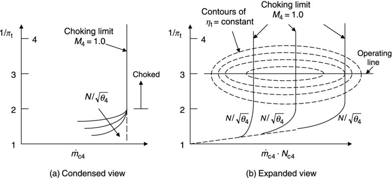
FIGURE 10.49 Typical turbine performance map
10.4 The Effect of Cooling on Turbine Efficiency
The impact of cooling on turbine efficiency may be attributed to the following effects:
- The coolant mass flow rate does not participate in turbine power production; therefore, per 1% cooling fraction there is ∼1% loss in power production (due to loss of working fluid)
- The coolant injection in the hot gas stream causes mixing losses of two streams as well as an increase in profile drag loss on the blades (for disruption of flow on the blades, as in film holes)
- The coolant suffers a total pressure drop inside the cooling passages due to friction, turbulators, pins, and other roughness elements inside the cooled turbine blades. The reduced total pressure on the part of the coolant then causes the stage total pressure ratio πt to drop
- The heat transfer between the hot gas and the coolant causes an entropy rise for the mixed-out gas.
The turbine efficiency may be defined as the ratio of actual turbine work per total airflow (that includes the coolant fraction) and the ideal turbine work, achieved isentropically, across the actual turbine expansion, (pt5/pt4)actual.
The actual turbine work (per unit mass flow) for the two streams is the sum of individual streams reaching the same exit total temperature Tt5
The ideal (i.e., isentropic) turbine work for the two streams expanding through the actual pressure ratio is
Therefore, the cooled turbine efficiency may be written as
Kerrebrock (1992) shows that turbine efficiency in Equation 10.87 may be approximated by

Where σ is the blade solidity, Stanton number is St, and Δpf is the total pressure loss due to riction inside the blade cooling passages. Kerrebrock estimates the loss o turbine efficiency to be ∼2.7% per percent of cooling flow for a typical gas turbine, based on Equation 10.88. Accounting for other sources of loss as in kinetic energy loss in film-cooled blades, Kerrebrock estimates an additional 1/2% to be added to the 2.7% to get an estimated 3.2% turbine efficiency loss per percent of cooling flow. More experimental data and validation are needed to cover a wide array of internal cooling configurations and internal/external loss estimation. Figure 10.50 shows the evolution of turbine blade cooling (courtesy of Rolls-Royce plc, 2005).

FIGURE 10.50 The evolution of turbine blade cooling. Source: Reproduced with permission from Rolls-Royce plc
10.5 Turbine Blade Profile Design
A definition sketch of a turbine cascade is shown in Figure 10.51. The basic parameters are the same as the compressor cascade. For example, the net flow turning is the difference between the inlet and exit flow angles (β1 and β2), or the camber angle (ϕ) is defined as the sum of the angles of the tangent to the mean camber line at the leading and trailing edge (κ1 and κ2). Also note that the deviation angle is the flow angle beyond the tangent to the mean camber line at the trailing edge (δ*). The blade setting or stagger angle is defined the same way as in a compressor cascade γo. The blade chord and spacing are the same as c and s, respectively. Now, let us examine some of the distinguishing features in a turbine cascade, such as an inlet induced flow angle Δθind, or throat opening o, or the suction surface curvature e, downstream of the throat, and finally the trailing-edge thickness tt.e.

FIGURE 10.51 Definition sketch of a turbine cascade
10.5.1 Angles
In order to construct a suitable turbine blade profile, we need to estimate the inlet and exit blade angles and their relation to the actual incidence and deviation angles. The incidence angle in a turbine cascade accounts for the flow curvature near the leading edge, called the induced turning, Δθind and is called actual incidence iac. The correlation between the induced angle, inlet flow angle, and blade solidity is (from Wilson and Korakianitis, 1998)
The actual incidence and flow angles are corrected by the induced angle according to
The flow and turbine blade angles at the leading edge follow the same relation as the compressor, that is,
The deviation angle is also important to the turbine profile design, as it adds to the blade camber, and if it is underpredicted, the exit swirl will be less than the design value and thus blade torque and in case of rotor, power, will be less than expected. Carter’s rule for deviation angle in a turbine, although not the most accurate, is adequate for the preliminary design purposes,
Stagger, or blade setting, angle is critical to the smoothness of turbine flow passage (area distribution) design. The simple approximation equates the stagger to the mean flow angle in a blade row, that is,
A more accurate determination of the stagger angle, based on the blade leading and trailing-edge angles, κ1 and κ2 is shown in Figure 10.52 (from Kacker and Okapuu, 1981).

FIGURE 10.52 Turbine blades stagger in relation to blade leading and trailing-edge angles. Source: Kacker and Okapuu 1981. Reproduced with permission from ASME
10.5.2 Other Blade Geometrical Parameters
Conventional turbine blade passages have their throat at the exit, as shown in Figure 10.51. It is desirable to expand the flow beyond the throat on the suction surface, that is, provide a convex curvature beyond the throat. This geometrical feature is advantageous to favorable pressure gradient and thus smaller deviation angle. The nondimensional radius of curvature s/e characterizes the convex curvature. The upper value for the convex curvature parameter s/e is 0.75 with typical range corresponding to 0.25 ≤ s/e ≤ 0.625. Also note that the pressure surface at the trailing edge assumes a concave curvature of radius ∼ (e + o).
In a turbine, the blade leading-edge radius r1.e. is critical to effective cooling and thus blade life. The value of nondimensional leading-edge radius r1.e./s is between 0.05 and 0.10.
The trailing-edge thickness, tt.e., in a turbine is finite. The main reasons are structural integrity as well as trailing-edge coolant slots. The trailing-edge thickness adversely impacts the flow blockage and blade profile losses. Thus, we wish to minimize the trailing-edge thickness consistent with the blade structural and cooling requirements. The typical non-dimensional values of tt.e./c fall between 0.015 and 0.05.
10.5.3 Throat Sizing
The throat sizing in a turbine nozzle (or rotor) is very important both for choked and unchoked nozzles. The geometry that is shown in the following definition sketch (Figure 10.53) is used to relate the throat width or opening o to the blade spacing s.

FIGURE 10.53 Definition sketch used for a turbine nozzle throat sizing
The throat opening o is related to the spacing and cosine of the exit flow angle α2 in nozzle and β2 in rotor, following
This approximation is acceptable for the subsonic exit flow, however, for the supersonic exit Mach numbers (but below 1.3), we correct the throat opening by the inverse of A/A* corresponding to the supersonic exit Mach number, that is,
The design exit Mach number for the first turbine nozzle should slightly exceed 1, that is, M2 > 1, and is commonly taken to be ∼ 1.1. The exit Mach numbers from the subsequent blades (in relative-to-blade frame of reference) in a turbine should remain below 1, that is, unchoked. For example, the design Mach number at the first rotor exit M3r is chosen to be as high as 0.90, but never 1 or above. Also, all subsequent blades in a multistage turbine, on the same spool, remain unchoked. For multispool gas turbines, the first nozzle, on all spools, is choked and its design exit Mach number is ∼1.1.
10.5.4 Throat Reynolds Number Reo
The throat Reynolds number should preferably be in the range of 105–106. Experimental data demonstrate a strong correlation between blade profile loss and the throat Reynolds number. The definition of throat Reynolds number uses the relative exit flow velocity from the blade and the static conditions at the throat, that is,
The throat opening o is given a subscript n and r in the above definitions, to signify the nozzle and rotor throat openings, respectively.
10.5.5 Turbine Blade Profile Design
We have identified some definite structure for the turbine profile at and beyond the throat. For example, we have the throat opening o/s related to exit flow angle and Mach number, or we have a range for the trailing-edge thickness, also a curvature on the suction side and a curvature on the pressure side, all near the trailing edge. At the leading edge, we have some design guidelines for the leading-edge radius, and some correlations for the induced flow turning, besides the flow angles at the inlet and exit. The stagger angle is also estimated using Equation 10.94 or Figure 10.51.
Once the trailing-edge passage beyond the throat is constructed and the leading-edge radius (or a range of radii) is chosen, the trial-and-error phase of curve fitting to the upper and lower surfaces begins. The goal is to produce a flow passage that smoothly and uniformly contracts to the throat section. Therefore, beyond the trailing-edge construction of the turbine blade profile, the rest of the approach deals with flow passage design (i.e., with a smooth area contraction).
Wilson and Korakianitis (1998) constructed the following turbine profile (Figure 10.54) based on the input shown in the box and the methodology of this section. Schobeiri (2004) also provides details in the construction of turbine profiles and is recommended for further reading.

FIGURE 10.54 Example of a turbine blade profile design. Source: Wilson and Korakianitis 1998. Reproduced with permission from the authors
10.5.6 Blade Vibration and Campbell Diagram
The Campbell diagram is of interest because it shows possible matches between blade vibrational mode frequency and multiples of shaft rotational speed. The multiples of shaft rotational speeds are caused by the struts and blades (wakes) in neighboring rows and they serve as the source of excitation. In essence, the blade passing frequency, which is the product of the number of blades times the shaft frequency, is the source of excitation for the blades in the next/previous row. Vibration frequency in kilohertz for the first two bending and the first two torsional modes is shown in Figure 10.55 (from Wilson and Korakianitis, 1998) to vary with rotor shaft speed (in rpm), due to the so-called stiffening effect that rotation has on a structure. The design shaft speed is also identified on the chart (to be ∼ 37, 000 rpm). The straight lines corresponding to multiple shaft speeds are drawn. The first or fundamental bending mode, known as the first-flap mode, has a natural frequency that lies between the fourth and sixth multiples of shaft rpm at design speed. Since the fifth multiple of shaft speed lies halfway between the fourth and sixth, we note that the first bending mode is below the fifth multiple of shaft speed at design rpm. Closer examination of Figure 10.54 also indicates that 4, 23, and 31 multiples of shaft speeds have a special significance in this turbine (rotor) blade row. These correspond to the number of struts and stator or nozzle blades that serve as the excitation source for the rotor through blade passing frequency of wakes and mutual interference effects of their rotating pressure fields.

FIGURE 10.55 Campbell frequency diagram for a turbine blade. Source: Wilson and Korakianitis 1998. Reproduced with permission from the authors
The structural design of blades should clearly indicate a resonance-free operating condition at the design speed, idle speed, and other operational speeds where significant time is spent. However, it is impossible to avoid all resonant frequencies as we speed up to the design, or other operational shaft speeds. Therefore, spool-up speed/acceleration, or the spool-down speed/deceleration are important to the cyclic loads and fatigue life of blades, struts, disks, and other engine components.
10.5.7 Turbine Blade and Disk Material Selection and Design Criteria
Turbine blade and disk materials and the year of development are shown in Figure 10.56 (from Wilson and Korakianitis, 1998). These, by necessity, are high-temperature materials. Some have high thermal conductivity, as in nickel-based alloys for the blades and disks thermal stress alleviation, and some are low thermal conductivity materials, such as ceramics, that reduce heat transfer to the blades. All materials, especially for turbine blades, use a thermal protection coating to reduce the surface operating temperature and thus in effect increase component life.

FIGURE 10.56 Turbine materials development. Source: Wilson and Korakianitis 1998. Reproduced with permission from the authors
There are four clusters of materials that are labeled in Figure 10.56. The conventional alloys exhibit the lowest operating temperature capability, whereas directional materials that include single crystals, rapid solidification rate alloys, oxide-dispersion-strengthened superalloys, and Tungsten–fiber superalloys achieve high temperature capability. The ceramics as in silicon carbide offer an additional tolerance to high temperature. The coated carbon–carbon composite material offers the highest temperature capability but the issues of cost, damage tolerance, inspectability, and reliability hamper its use in large operational gas turbine engines. The turbine design example at the end of this chapter uses a design blade surface temperature of 1400 K, which based on Figure 10.56 implies the use of directionally solidified material.
Different parts of turbine blade and disk are subject to different mechanical design criteria, as shown in Figure 10.57 (from Wilson and Korakianitis, 1998). Mechanical designs of turbine components address low- and high-cycle fatigue, oxidation/corrosion, and creep rupture problems.
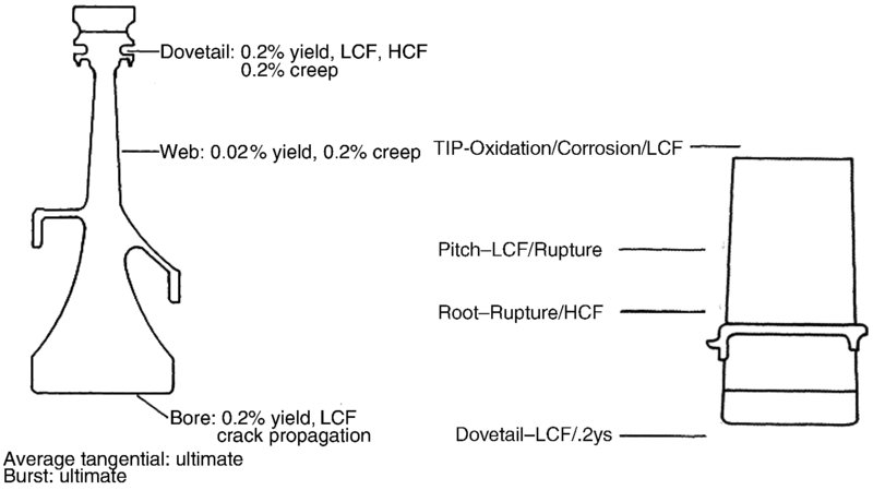
FIGURE 10.57 Different design criteria for turbine blade and disk (LCF: low-cycle fatigue HCF: high-cycle fatigue, YS: yield strength). Source: Wilson and Korakianitis 1998. Reproduced with permission from the authors
The number of cycles to failure for conventionally cast and directionally solidified material shows the fatigue strength of Rene 80, directionally solidified Rene 150, and directionally solidified Eutectic material (that are typically used in turbine blades) in Figure 10.58 (from Wilson and Korakianitis, 1998). We note that directional solidification improves fatigue strength by a factor of 2 or 5 over conventionally cast Rene 80 as shown in Figure 10.58.

FIGURE 10.58 Fatigue strength of turbine blade material. Source: Wilson and Korakianitis 1998. Reproduced with permission from the authors
Another material characteristic of interest to turbine designers is the creep rupture strength. It is the maximum tensile stress that material tolerates without failure over a time period at a given temperature. The 0.2% creep design criterion is listed for the turbine disk web, blade slot in the hub, blade pitchline, and root. This 0.2% creep rupture strength is plotted for three materials that are used in turbine disks in Figure 10.59 (from Wilson and Korakianitis, 1998). The temperature (in Kelvin) and time (in hours) are combined in the Larson-Miller parameter on the abscissa of Figure 10.59. The Larson–Miller parameter is defined as
Where C is constant for a material (in this case, 25).

FIGURE 10.59 0.2% Creep strength of turbine disk alloys. Source: Wilson and Korakianitis 1998. Reproduced with permission from the authors
The treatment of the turbine material selection and design criteria in this section has been by necessity very brief. We have not even scratched the surface of the vast and specialized field of gas turbine high-temperature materials and mechanical design. The reader is to refer to specialized texts and references on the subject.
10.6 Stresses in Turbine Blades and Disks and Useful Life Estimation
Turbine blades and disks are subjected to centrifugal stresses due to shaft rotation as well as thermal stresses due to temperature differentials in the material due to cooling, gas bending stresses due to gas loads, and vibratory stresses due to cyclic loading and blade vibration. The centrifugal stresses take on the same form as the one developed in the compressor section.
The dominant stress in a rotor and disk is the centrifugal stress σc. At the blade hub, the ratio of the centrifugal force Fc to the blade area at the hub Ah is the centrifugal stress, σc,

The blade area distribution along the span Ab(r)/Ah is known as taper and is often approximated to be a linear function of the span. Therefore, it may be written as
We may substitute Ab(r)/A in the integral and proceed to integrate; however, a customary approximation is often introduced that replaces the variable r by the pitchline radius rm. The result is
Therefore, the ratio of centrifugal stress to the material density is related to the square of the angular speed, the taper ratio, and the flow area, A = 2πrm(rt − rh). This equation is the basis of the so-called AN2 rule, that is, where A is the flow area and N is the shaft angular speed, often expressed in the customary unit of rpm. The right-hand side of Equation 10.105 incorporates turbomachinery size (throughflow area) and the impact of angular speed, whereas the left-hand side of Equation 10.105 is a material property known as the (tensile) specific strength.
The material parameter of interest in a rotor is the creep rupture strength, which identifies the maximum tensile stress tolerated by the material for a given period of time at a specified operating temperature. Based on the 80% value of the allowable 0.2% creep in 1000 h, for aluminum alloys and the 50% value of the allowable 0.1% creep in 1000 h for other materials, Mattingly, Heiser, and Pr and 10.61. They show the allowable stress and the allowable specific strength of different engine materials as a function of temperature. Note that the unit of stress in the following two figures is ksi, which is 1000 lb per square inch (i.e., 1000 psi) and the temperatures are expressed in degree Fahrenheit.

FIGURE 10.60 Allowable stress versus temperature for typical engine materials. Source: Mattingly, Heiser, and Pratt 2002. Reproduced with permission from AIAA

FIGURE 10.61 Allowable strength-to-weight ratio for typical engine materials. Source: Mattingly, Heiser, and Pratt 2002. Reproduced with permission from AIAA
Thermal stresses are calculated based on thermal strains that are set up in a material with differential temperature ΔT from
where ![]() t is thermal strain (i.e., elongation per unit length) and α is the coefficient of (linear) thermal expansion, which is a material property. The linear stress–strain relationship demands
t is thermal strain (i.e., elongation per unit length) and α is the coefficient of (linear) thermal expansion, which is a material property. The linear stress–strain relationship demands
where E is the modulus of elasticity. The thermal stresses in a disk of constant thickness with no center hole and with the radius rh is a simple model of a turbine disk. If the disk has a linear temperature distribution in the radial direction, the thermal stresses in radial and tangential directions are shown (by Mattingly, Heiser, and Pratt, 2002) to be


The maximum of both stresses occur at the center of the disk, that is, r = 0, and for typical values of coefficient of thermal expansion of nickel-based alloys, α ∼ 10.2 × 10⁻⁶ in/in.oF at 1400 oF (that corresponds to gas turbine temperatures), as well as the modulus of elasticity E for nickel alloys (at 1400 °F) is ∼ 20.5 × 10⁶ psi, which for a 100 °F temperature differential gives thermal stresses in the radial and tangential directions of about ∼ 6970 psi (equivalent to 1011 kPa). This example illustrates the need for special attention to the thermal stresses in turbine disks and material property that is of utmost interest is the thermal conductivity. The transient operations of the gas turbine that expose the turbine disk to high temperatures at the rim while the center of the disk is still at a low temperature pose the highest levels of thermal stress. Nickel alloys have the highest levels of thermal conductivity, in metals, at high temperatures, which are suitable for use in turbine disks and blades.
The total stress in the material, σtotal, which is the sum of the centrifugal, bending (i.e., gas loads), thermal and vibratory stresses, and the material operating temperature combine to estimate material (useful) life. There are stress–temperature–material life curves, for a variety of materials, in gas turbine industrial practice. Figure 10.62 shows an example of a family of stress–temperature–life curves for any given material, for example, nickel alloys.

FIGURE 10.62 Material (useful) life curves
10.7 Axial-Flow Turbine Design and Practices
In this section, we apply some of the concepts that we learned in the chapter to the preliminary design of a cooled gas turbine. The approach to turbine design is as varied and diverse as the textbooks written on the subject. Therefore, there is no unique approach to turbine design, rather the author’s preference in applying a set of guidelines to turbine design.

FIGURE 10.63 Definition sketch of a two-stage turbine and its station numbers
10.8 Gas Turbine Design Summary
We used some commonly accepted design practices, for example, constant axial velocity, to design suitable velocity triangles at the pitchline. In the process, we encountered some hard and soft design constraints. Some examples of hard and soft design constraints are summarized below:
| Hard design constraints | Soft design constraints | ||
| M2 > 1 | (choked first nozzle) | σ ≠ σopt | (solidity other than the optimum) |
| M3r < 1 | (unchoked rotor exit flow) | rm ≠ constant | (pitchline radius is variable) |
| M5r < 1 | (unchoked rotor exit flow) | αexit ≠ 0 | (turbine exit swirl not zero) |
| Twg | (maximum wall temperature) | twall = 2 mm | (wall thickness other than nominal) |
| °R > 0 | (positive degree of reaction) | 0 ≤ °R ≤ 1 | (wide-ranging choice of °R) |
| Twg = 1400 K | (a function of material selection) | ||
| ψ > 1 | (higher loading than 1 is acceptable) | ||
| Cz ≠ constant | (acceptable) | ||
| η ≈ 0.6–0.7 | (cooling effectiveness for | ||
| film + conv. cooling) | |||
| η < 0.4 | (cooling effectiveness for | ||
| internal conv. cooling) | |||
| Tc < 900 K | (limited by comp. discharge) |
The design process requires iteration. To facilitate successive calculations, a spreadsheet was developed. It is important to recognize the approximations that were used in the analysis. For example, we used the same Tc in our internal cooling calculations for the nozzle and the rotor. The coolant temperature that we used in the nozzle was the compressor discharge temperature. However, when the coolant is injected in the hub of a rotating blade row, as in the rotor, the relative stagnation temperature is different than the absolute total temperature. But, we did not distinguish between the two. In practice, the coolant is injected at an angle in the direction of rotor rotation with the resultant relative stream in the axial direction. The schematic drawing of a cooled turbine rotor blade and the coolant velocity triangle is shown in Figure 10.64 The correction for the coolant relative total temperature is shown to be ∼ ![]() . Therefore, the coolant entering the blade root feels cooler to the rotor than the coolant in the nozzle. Here, the emphasis in the summary is not on the extent of correction to the stagnation temperature, rather on the awareness of the two frames of reference.
. Therefore, the coolant entering the blade root feels cooler to the rotor than the coolant in the nozzle. Here, the emphasis in the summary is not on the extent of correction to the stagnation temperature, rather on the awareness of the two frames of reference.

FIGURE 10.64 Definition sketch for coolant entry at the rotor blade root and coolant total temperature in the rotor frame of reference
Figure 10.65 shows a flowchart in turbine design based on the methodology presented in this chapter. The flowchart shows a two-stage turbine with cooling fractions, ![]() N1,
N1, ![]() R1, and so on, shown in the right-hand column. The middle column shows the design input parameters in uncooled turbine blade rows as the exit Mach number and flow angles. The left-hand column shows the flow cross-sectional area sizing based on continuity.
R1, and so on, shown in the right-hand column. The middle column shows the design input parameters in uncooled turbine blade rows as the exit Mach number and flow angles. The left-hand column shows the flow cross-sectional area sizing based on continuity.

FIGURE 10.65 Flowchart for a cooled two-stage turbine calculation strategy and sizing procedure
10.9 Summary
Modern gas turbines truly represent the most technologically challenging component in an aircraft engine. Critical technologies in the development of gas turbines are (single crystal) material, internal/external cooling, thermal protection coating, aerodynamics, active tip clearance control, and manufacturing.
Degree of reaction in a turbine influences power production, efficiency, and stage mass flow density (i.e., mass flow rate per unit area). For example, a 50% reaction turbine stage produces (for a swirl-free rotor exit flow)
And an impulse turbine (with 0% reaction) stage produces (for a swirl-free rotor exit flow)
The choice of nozzle optimal exit swirl Mach number coupled with axial flow from the rotor demonstrated that the choice of degree of reaction establishes a turbine inlet Mach number M1. An impulse turbine stage, with °R = 0, demands a nozzle inlet Mach number of ∼ 0.4 and a 50% reaction stage corresponds to an inlet Mach number ∼ 0.65. With the increase in reaction, the mass flow rate per unit area increases and vice versa. Although an impulse stage is capable of producing maximum specific work, it also reduces the mass flow density. The optimal nozzle exit Mach number M2 that maximizes the swirl and stage work varies between 1.2 and 1.5 for a stage reaction that varies between 50% and 0, respectively. The practical maximum exit flow angle in a nozzle is α2, max ≈ 70°.
Turbine losses are attributed to the following sources:
- Profile loss, which is established based on 2D cascade studies
- Secondary flow losses, which may be estimated using secondary flow theory of Hawthorne or the approximate version by Squire and Winter
- Annulus losses, which includes tip clearance loss, (seal) leakage loss, casing boundary layer loss, corner vortex loss
- Coolant-related losses, including mixing loss, induced separation loss, and internal passage coolant total pressure loss
- Shock and shock-boundary layer interaction losses in transonic stages of LPT
- Unsteady flow loss causing shock oscillation and vortex shedding in the wake.
In examining blade profile losses, we have noted that the impulse blade profile losses are significantly higher than their counterparts in a reaction rotor. This contributes to lower stage efficiency in an impulse type versus a reaction turbine. Tip clearance is a major contributor to turbine losses, and consequently the active control of tip clearance is an adopted/practiced strategy. The other option is to shroud the turbine rotor blades (at the tip) to eliminate the tip clearance loss. The added weight and centrifugal stresses in shrouded rotors are the penalty paid for such a relief.
We introduced the concept of optimal solidity in turbine aerodynamics. However, the two criteria for optimum solidity, that is, Zweifel’s and Howell’s, showed a very limited range of agreement with the test data.
Turbine cooling relies on internal and external cooling schemes as well as thermal protection coating. Leading-edge impingement and internal convective cooling are practiced internally. Either film or transpiration cooling achieves the external cooling. The role of the thermal protection coating is to reduce the heat transfer to the blade by coating the blades with a very low thermal conductivity layer (as in silicon-based paint, or ceramic coating).
Glassman (1973), Hill and Peterson (1992), Marble (1964) and Schobeiri (2004) are recommended for additional reading on gas turbines. VKI Lecture series (1982) and Glass, Dilley and Kelly (1999) provide valuable discussions on advanced turbine cooling. The contributions of Garvin (1998) and St. Peter (1999) on the history of gas turbine development in the United States are also recommended.
References
- Ainley, D.G., “An Approximate Method for Estimation of the Design Point Efficiency of Axial Flow Turbines, ” British Aeronautical Research Council Current Paper 30, 1950.
- Ainley, D.G. and Mathieson, G.C.R.“A Method for Performance Estimation for Axial Flow Turbines, ” Aeronautical Research Council, Research and Memorandum No. 2974, 1951.
- Anderhub, W., “Untersuchungen ueber die Dampfstroemung im radialen Schaufelspalts bei Ueberdruckturbinen, ” Doctoral Dissertation, Swiss Federal Institute of Technology, Zurich, Switzerland, 1912.
- Bammert, K., Klaeukens, H., and Hartmann, D., “Der Einfluss des radialen Schaufelspalts auf den Wirkungsgrad mehrstufige Turbinen, ” VDI-Zeitschrift, Vol. 110, No. 10, April 1968, pp. 390–395.
- Booth, T.C., Dodge, P.R., and Hepworth, H.K., “Rotor Tip Leakage: Part I-Basic Methodology, ” Transactions of ASME, Journal of Engineering for power, Vol. 104, January 1982, pp. 154–161.
- Colladay, R.S., “Turbine Cooling, ” A Chapter in Turbine Design and Applications, Glassman, A.J. (Ed.), NASA SP-290, Washington, DC, 1975.
- Dixon, S.L., Fluid Mechanics, Thermodynamics of Turbomachinery, 2nd edition, Pergamon Press, Oxford, UK, 1975.
- Duncombe, E., “Aerodynamic Design of Axial Flow Turbines, ” Section H, in Aerodynamics of Turbines and Compressors, Vol. X, Hawthorne, W. R. (Ed.), Princeton Series on High Speed Aerodynamics and Jet Propulsion, Princeton University Press, Princeton, NJ, 1964.
- Dunham, J. and Came, P., “Improvements to the Ainley-Mathieson Method of Turbine Performance Predic-tion, ” Transactions of the ASME, Series A, Vol. 92, 1970.
- Eckert, E.R.G., Analysis of Heat and Mass Transfer McGraw-Hill, New York, 1971.
- Eckert, E.R.G. and Livingood, N.B., “Comparison of the Effectiveness of Convection-, Transpiration-, and Film-Cooling Methods with Air as Coolant, ” NACA Report 1182, 1953.
- Farokhi, S., “The Effect of Rotor Tip Clearance Flow on the Axial Exhaust Diffuser and the Turbine Performance, ” Proceedings of the First International Power Conference in Beijing-China, October 1986, pp. 348–353.
- Farokhi, S., “A Trade-Off Study of Rotor Tip Clearance Flow in a Turbine/Exhaust Diffuser System, ” ASME Paper No. 87-GT-229, June 1987.
- Farokhi, S., “Analysis of Rotor Tip-Clearance Loss in Axial Flow Turbines, ” AIAA Journal of Propulsion and Power, Vol. 4, No. 5, September–October 1988, pp. 452–457
- Garvin, R.V., Starting Something Big: The Commercial Emergence of GE Aircraft Engines, AIAA, Inc., Reston, VA, 1998.
- Glass, D.E., Dilley, A.D., and Kelly, H.N., “Numerical Analysis of Convection/Transpiration Cooling, ” NASA/TM-1999-209828, 1999.
- Glassman, A.J. (Ed.), Turbine Design and Application, 3 volumes, NASA SP-290, 1973.
- Graham, J.A.H., “Investigation of Tip Clearance Cascade in a Water Analogy Rig, ” Transactions of ASME, Journal of Engineering for Gas Turbines and Power, Vol. 108, January 1986, pp. 38–46.
- Gostelow, J.P., Cascade Aerodynamics, Pergamon Press, Oxford, UK, 1984.
- Hawthorne, W.R., “Secondary Circulation in Fluid Flow, ” Proceedings of Royal Society, London, Vol. 206, 374, 1951.
- Hill, P.G. and Peterson, C.R., Mechanics and Thermo-dynamics of Propulsion, 2nd edition, Addison-Wesely, Reading, MA, 1992.
- Incropera, F.P. and DeWitt, D.P., Fundamentals of Heat and Mass Transfer, 5th edition, John Wiley & Sons, Inc., New York, 2001.
- Johnston, I.H., “An Analysis of Air Flow Through the Nozzle Blades of a Single Stage Turbine, ” ARC Current Paper 131, 1953.
- Kacker, S.C. and Okapuu, U., “A mean-line prediction method for axial-flow-turbine efficiency, ” Paper no. 81- GT-58, ASME, New York, 1981.
- Kercher, D.M. and Tabakoff, W., “Heat Transfer by a Square Array of Round Air Jets Impinging Perpendicular to a Flat Surface Including the Effect of Spent Air, ” ASME Journal of Engineering for Power, Vol. 92, No. 1, January 1970, pp. 73-82.
- Kerrebrock, J.L., Aircraft Engines and Gas Turbines, 2nd Edition, MIT Press, Cambridge, MA, 1992.
- Lakshminarayana, B., “Methods of Predicting the Tip Clearance Effects in Axial Flow Turbomachinery, Transactions of ASME, Journal of Basic Engineering, Vol. 92, September 1970, pp. 467–482.
- Mattingly, J.D., Heiser, W.H., and Pratt, D. T., Aircraft Engine Design, 2nd Edition, AIAA Education Series, AIAA, Reston, VA, 2002.
- Marble, F.E., “Three-Dimensional Flow in Turbomachines, in, Aerodynamics of Turbines and Compressors, Vol. X, Hawthorne W.R. (Ed.), Princeton Series on High Speed Aerodynamics and Jet Propulsion, Princeton University Press, Princeton, NJ, 1964.
- Rohsenow, W.M., Hartnett, J.P., and Cho, Y.I., Handbook of Heat Transfer, 3rd edition, McGraw-Hill, New York, 1998.
- Rolls-Royce, The Jet Engine, Rolls-Royce plc, Derby, UK, 2005.
- Schobeiri, M., Turbomachinery Flow Physics and Dynamic Performance. Springer Verlag, Berlin, 2004.
- St. Peter, J., The History of Aircraft gas Turbine Engine Development in the United States, International Gas Turbine Institute, Atlanta, GA, 1999.
- Stodola, A., Dampf- und Gasturbinen, Springer Verlag, 1924.
- Stodola, A., Steam and Gas Turbines, Vols. 1 and 2, McGraw-Hill, New York, 1927.
- Traupel, W., Thermische Turbomaschinen, Vol. 1, Springer Verlag, 1958, pp. 295–296.
- VKI-Lecture Series, “Film Cooling and Turbine Blade Heat Transfer, ” VKI-LS 82-02, 1982.
- Wang, J.H., Messner, J., and Stetter, H., “An Experimental Investigation on Transpiration Cooling Part II: Comparison of Cooling Methods and Media, “ International Journal of Rotating Machinery, Vol. 10, No. 5, 2004, pp. 355–363.
- Wilson, D.G. and Korakianitis, T. The Design of High-Efficiency Turbomachinery and Gas Turbines, 2nd edition, Prentice Hall, New York, 1998.
- Zweifel, O., “The Spacing of Turbomachine Blading, Especially with Large Angular Deflection, ” Brown Boveri Review, Vol. 32, No. 12, December 1945, pp. 436–444.
Problems
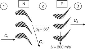
- 10.1 The combustor discharge into a turbine nozzle has a total temperature of 1850 K and inlet Mach number of 0.50, as shown.

Assuming that the nozzle is uncooled, the axial velocity remains constant across the nozzle and the absolute flow angle at the nozzle exit is α2 = 65°, calculate
- inlet velocity C1 in m/s
- the exit absolute Mach number M2 and
- nozzle torque per unit mass flow rate for r1 ≈ r2 = 0.40 m
- 10.2 Calculate the nozzle exit flow angle α2 in Problem 10.1, if we wish the exit Mach number to be M2 = 1.0, i.e., choked.
- 10.3 A turbine stage at pitchline has the following velocity vectors, as shown.

Calculate:
- the axial velocities up- and downstream of the rotor
- relative flow angle β2 in degrees
- the rotor velocity Um
- the degree of reaction at this radius
- rotor specific work, wm in kJ/kg
- 10.4 A turbine stage is designed with a constant axial velocity of 250 m/s and zero exit swirl. For a rotor rotational speed Um at the pitchline of 600 m/s.
Calculate
- the nozzle exit flow angle, α2 in degrees for °Rm = 0.50
- the nozzle exit flow angle, α2 in degrees for °Rm = 0.0
- the rotor specific work at the pitchline radius, for °Rm = 0.50 and °Rm = 0.0
- 10.5 An axial-flow turbine nozzle turns the flow from an axial direction in the inlet to an exit flow angle of α2 = 70°. The rotor wheel speed is U = 400 m/s at the pitchline. The rotor is of impulse design and the exit flow from the rotor has zero swirl, i.e., α3 = 0. Calculate
- the rotor-specific work
- the stage loading at the pitchline
- 10.6 An axial-flow turbine stage at the pitchline is shown.
The flow entering and exiting the turbine stage is axial, i.e., α1 = α3 = 0

The nozzle exit flow is α2 = 65°. The shaft speed is ω = 5500 rpm and the pitchline radius is rm = 50 cm. Assuming Cz = 250 m/s = constant.
Calculate
- turbine-specific work wt(kJ/kg)
- β3 (degrees)
- °Rm
- 10.7 The combustor discharge total temperature and pressure are Tt1 = 2000 K and pt1 = 2 MPa, respectively, with γt = 1.30 and cpt = 1244 J/kg · K. The flow speed is 400 m/s and is in the axial direction. Calculate
- the combustor exit static temperature T1 in K
- the Mach number M1
- the combustor exit static pressure p1 (in kPa)
- 10.8 The inlet flow condition to a turbine nozzle is characterized by Tt1 = 1800 K and pt1 = 2.4 MPa, M1 = 0.5, α = 5°, with γt = 1.30 and cpt = 1244 J/kg · K. Assuming the nozzle is designed for constant axial velocity, i.e., Cz = constant, calculate the nozzle exit flow angle α2 that will produce the exit Mach number of M2 = 1.1.
- 10.9 For the flow condition across a nozzle as shown, calculate
- T2 in K
- Cz2 in m/s
- Cθ2 in m/s
- M1
- pt2 in MPa
- p2 in kPa
Assume Cz = constant, γt = 1.30, and cpt = 1244 J/kg · K.

- 10.10 The velocity triangles across a turbine rotor are shown. The axial velocity remains constant across the rotor. If the total temperature at the rotor inlet is 1850 K with γt = 1.30 and cpt = 1244 J/kg · K, calculate

- inlet absolute Mach number M2
- inlet relative Mach number M2r
- the degree of reaction °R
- rotor specific work wt in kJ/kg
- exit static temperature T3(K)
- exit relative Mach number M3r.
- 10.11 A rotor is designed for constant axial velocity. The velocity triangles are as shown. The rotor total pressure loss coefficient is known to be 0.08 with γt = 1.30 and Rt = 287 J/kg · K.

Calculate
- rotor speed U in m/s
- rotor specific work wt in kJ/kg
- stage degree of reaction °R
- rotor circulation Γ in m2/s
- inlet absolute Mach number M2
- inlet gas static density ρ2 in kg/m3
- exit relative Mach number M3r
- exit total pressure pt3 in MPa
- exit static density ρ3 in kg/m3.
- 10.12 Coolant air is bled from a compressor exit at Ttc = 800 K with cpc = 1004 J/kg · K. The coolant is given a (positive) preswirl before it enters the rotor blade root in the direction of the rotor rotation. Assuming the port of coolant entry into the rotor is at rc = 42 cm with rotor angular speed ω = 12000 rpm, and the coolant enters the rotor blade root axially, as shown in Figure 10.64, calculate the coolant relative total temperature as it enters the rotor blade.
- 10.13 A multistage turbine is to be designed with constant axial velocity. The total temperature ratio across the entire turbine is τt = 0.72 and the turbine polytropic efficiency is et = 0.85 with γt = 1.30 and cpt = 1244 J/kg · K. Calculate
- The turbine total pressure ratio πt
- the turbine adiabatic efficiency ηt
- turbine area ratio, A5/A4, for choked inlet, i.e., M4 = 1.0, Tt4 = 1675 K and Cz = 445 m/s and swirl-free exit flow
Assume γ and R remain constant across the turbine.
- 10.14 A 50% degree of reaction turbine stage is shown. The nozzle turns the flow 65° and the rotor exit flow is swirl-free. Assuming axial velocity remains constant throughout the stage, calculate
- axial velocity Cz m/s
- rotor specific work wt kJ/kg
- stage loading ψ
- flow coefficient ϕ
- static temperature drop ΔT = T1 − T2
- static temperature drop ΔT = T2 − T3
Assume cpt = 1.156 kJ/kg · K.
- 10.15 A simple method to establish the annulus geometry in a multistage turbine is to assume a constant throughflow (i.e., axial) speed Cz. Calculate
- the density ratio ρ5/ρ4
- the exit-to-inlet area ratio A5/A4
for

Also, if the hub radius is constant, calculate the tip-to-tip radius ratio (r5/r4)tip for (rh/rt)4 = 0.80

- 10.16 A turbine stage has an inlet total temperature Tt1 of 2000 K. If the rotational speed of the rotor at the pitchline is 200 m/s and the axial velocity component is Cz = 250 m/s, calculate
- the stagnation temperature as seen by the rotor, Tt2, r
- the gas static temperature upstream of the rotor, T2
- the adiabatic wall temperature for the rotor, Taw, r assuming a turbulent boundary layer
Assume γ = 1.33, cp = 1156 J/kg · K and Pr = 0.71.

- 10.17 A turbine stage is characterized by a loading coefficient, ψ of 0.8, and a flow coefficient of
 of 0.6. The rotor is unshrouded and has a tip clearance gap-to-blade height ratio of 2.5%. The ratio of the tip to pitchline radius is rt/rm = 1.50. The rotor blade tip has a knife configuration with a tip discharge coefficient of 0.60. The mean relative flow angle in the turbine rotor is βm = −30°. Calculate the loss of turbine efficiency due to the tip clearance.
 - 10.18 The relative flow angles in a turbine rotor are β2 = 25° and β3 = −45°.
Calculate
- optimum axial solidity parameter
- the axial solidity σz based on the recommended value of the loading coefficient ψz
- 10.19 The thermal boundary layer associated with the flow of a hot gas over an insulated flat plate is shown.
Assume that the gas Prandtl number is Pr = 0.71, the ratio of specific heats is γ = 1.33, the gas Mach number is Mg = 0.75.

Calculate
- the adiabatic wall temperature Taw in K
- the gas stagnation temperature Ttg in K
First assume that the viscous boundary layer is laminar and then solve the problem for a turbulent boundary layer.
- 10.20 Consider the flow of high-temperature, high Mach number gas over a flat wall, (Mg = 1.0, γg = 1.33, cpg = 1156 J/kg · K,
 ). We intend to internally cool the wall to achieve a wall temperature of Twg = 1200 K.

Assuming the gas-side Stanton number is Stg = 0.005, calculate
- the gas stagnation temperature Ttg K
- the adiabatic wall temperature Taw K for a turbulent boundary layer
- the gas-side film coefficient hg W/m2 K
- the heat flux to the wall qw kW/m2
For a wall thickness of tw = 3 mm, and a thermal conductivity, kw = 14.9 W/m · K, calculate
- the wall temperature on the coolant side Twc K
- 10.21 The leading edge on a turbine nozzle is to be internally cooled using an impingement cooling technique, as shown. The leading-edge diameter is 8 mm. Calculate the heat transfer coefficient hg at the leading edge, assuming an augmentation factor a = 1.5 due to a high-intensity turbulent flow in the turbine (use Equation 10.81 for a cylinder in cross-flow).

- 10.22 The exit flow angle in a turbine nozzle at the pitchline is 70°. The blade spacing is s = 6 cm. The total pressure and temperature at the nozzle throat are 2.6 MPa and 1700 K, respectively. Assuming the nozzle throat is choked calculate the mass flow rate (per unit span) through a single nozzle blade passage. The gas properties may be assumed to be γt = 1.30 and cpt = 1244 J/kg · K.
- 10.23 A turbine blade row is cooled with a coolant mass fraction of 3% and the coolant inlet temperature of Ttc = 775 K. The coolant is ejected at the blade trailing edge at a temperature of 825 K as it mixes with the hot gas at the temperature of 1825 K. Assuming gas properties for the coolant and hot gas are γc = 1.40, cpc = 1004 J/kg · K and γt = 1.30 and cpt = 1244 J/kg · K and the coolant flow rate is 3 kg/s, calculate
- the rate of heat transfer to the coolant from the blade in kW
- the mixed-out specific heat (of the coolant and the hot gas after mixing)
- the mixed-out temperature (of the coolant and the hot gas after mixing)
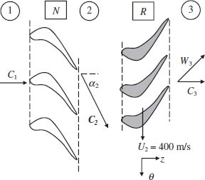
- 10.24 The total temperature and pressure at the entrance to a rotor are known to be 1850 K and 3.0 MPa, respectively. The rotor is of constant axial velocity design with Cz = 442 m/s. The rotor relative velocity at the inlet is W2 = 562 m/s. The rotor relative exit Mach number is to be M3r = 0.90. Assuming α2 = 60°, γ = 1.33 and cp = 1156 J/kg · K calculate
- the relative inlet Mach number M2r
- the relative flow angle at the exit β3 (degrees)
- the absolute exit flow angle α3 (degrees)
- stage degree of reaction °R
- 10.25 A turbine rotor has a tip clearance height of 1% compared with blade height. The loading coefficient is ψ = 2.5 and the flow coefficient is ϕ = 0.6. The turbine efficiency for zero tip clearance is η0 = 0.85. The tip-to-mean radius ratio is rt/rm = 1.25, and the mean flow angle in the rotor is βm = −15°. Using the following tip clearance efficiency loss model,

calculate the turbine efficiency loss due to 1% tip clearance for the following rotor tip shapes
- knife with gap Reynolds number of 2000
- groove
Assuming the rotor with a flat-tip has a discharge coefficient of CD, flat-tip = 0.83.
- 10.26 The free-stream gas temperature is T∞ = 1600 K and the free-stream gas speed is V∞ = 850 m/s. The gas properties are γt = 1.30, cpt = 1244 J/kg · K and Prandtl number Pr = 0.73. Consider the flow of this gas over a flat plate at a high Reynolds number corresponding to turbulent flow. Calculate
- the gas total temperature Tt∞ in K in the freestream
- the adiabatic wall temperature Taw in K
- percent error if we assume adiabatic wall temperature is the same as total temperature of the gas
- 10.27 A gas turbine is to provide a shaft power of 50 MW to a compressor with mass flow rate of 100 kg/s. The compressor bleeds 10 kg/s at its exit for turbine internal cooling purposes. The combustor exit mass flow rate is 93 kg/s, which accounts for 3 kg/s of fuel flow rate in the combustor. The turbine inlet temperature is Tt4 = 1850 K and pt4 = 2.0 MPa with γt = 1.30, cpt = 1244 J/kg · K Assuming the coolant total temperature is Ttc = 785 K and the gas properties are γc = 1.40, cpc = 1004 J/kg · K, calculate
- the turbine exit total temperature Tt5-cooled
- the turbine exit total pressure pt5-cooled.
You may assume that the effect of cooling on turbine adiabatic efficiency is about ∼2.8% loss (of efficiency) per 1% cooling.
- 10.29 The Stanton number is in general a function of Prandtl and Reynolds numbers, among other nondimensional parameters such as Mach number, roughness, curvature, free-stream turbulence intensity, etc. Eckert–Livingood model for a flat plate with constant wall temperature, excluding all other effects except Prandtl number and the Reynolds number, is

for a turbulent boundary layer. The Prandtl number for the gas is 0.704 and remains constant along the plate. Make a spreadsheet calculation of Stanton number Stg with respect to Reynolds number in the range of
 . Graph the Stanton number versus Reynolds number. Also, calculate the wall-averaged Stanton number.
 - 10.29 The nozzle throat opening o is to be sized for a throat Reynolds number of Reo = 500, 000. The throat is choked with Tt-throat = 2000 K, pt-throat = 2.1 MPa, and the gas properties at the throat are γt = 1.30, cpt = 1244 J/kg · K, μthroat = 6.5 × 10− 5kg/m · s. Calculate the nozzle throat opening o in centimeters.
- 10.30 A turbine rotor has a hub and tip radii

The rotor angular speed is ω = 2500 rpm. The rotor blade taper ratio At/Ah is 0.75. Estimate the ratio of blade centrifugal stress at the hub to blade material density, σc/ρblade. If this rotor operates at 1200°F, what are the suitable materials forthis rotor? (Hint: Use Figure 10.61 as a guide)
- 10.31 An uncooled turbine stage is of impulse design with °R = 0. The rotor exit is swirl free, i.e., Cθ3 = 0. The nozzle exit absolute flow angle is α2 = 70o. The axial velocity is constant throughout the stage and is equal to Cz = 252 m/s. The gas properties are: γt = 1.33 and cpt = 1, 156 J/kg · K. The turbine inlet total temperature is Tt1 = 1650 K. Calculate
- rotor (rotational) speed, U2, in m/s
- total temperature drop in the stage, ΔTt, in K
- speed of sound, a2, in m/s
- speed of sound, a3, in m/s
- absolute Mach number, M2
- relative rotor exit Mach number, Mr3

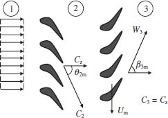
- 10.32 An axial-flow turbine stage, at its pitchline radius, is shown. The rotor exit is swirl free, i.e., Cθ3 = 0. The axial velocity is constant throughout the stage and is equal to Cz = 300 m/s. The flow to the turbine stage is purely axial, i.e., C1 = Cz1 and the gas total temperature is Tt1 = 1500 K with γt = 1.33 and cpt = 1, 156 J/kg · K. Assume that the turbine is uncooled and the stage degree of reaction is 20%. Calculate
- the nozzle exit flow angle, α2, in degrees
- the stage specific work in kJ/kg
- total temperature relative to the rotor, Tt2, r, in K
- absolute Mach number at nozzle exit, M2
- speed of sound, a3, in m/s
- relative rotor exit Mach number, M3r
- 10.33 A turbine stage at the pitchline is designed with 15% degree of reaction and zero exit swirl, as shown. The pitchline radius is at rm = 0.60 m and shaft rotational speed is ω = 6500 rpm. Assuming the axial velocity is constant; calculate the following parameters at the pitchline:
- nozzle exit absolute swirl, Cθ2, in m/s
- nozzle exit Mach number, M2
- rotor exit relative Mach number, M3r
- the stage loading at pitchline, ψm

- 10.34 A turbine stage is designed with constant axial velocity of Cz = 200 m/s. The absolute flow angle at the nozzle entrance is zero, i.e., α1 = 0o, and at the nozzle exit is α2 = 70o. Assuming the mass flow rate through the nozzle (blade row) is
 , and rm = 0.5 m, calculate
- (mean) torque acting on the nozzle blades in kN-m
- static temperature at the nozzle exit, T2, in K

- 10.35 An axial-flow turbine nozzle turns the flow from an axial direction in the inlet to an exit flow angle of α2 = 70o. The rotational speed of the rotor at the pitchline is U = 400 m/s. The exit flow from the stage is swirl free, i.e., α3 = 0. Assuming that the axial velocity is constant in the stage, Cz = 265 m/s, and the turbine inlet conditions are: Tt1 = 1750 K, pt1 = 2 MPa, γt = 1.33 and cpt = 1156 J/kg · K, calculate
- absolute swirl at the nozzle exit, Cθ2, in m/s
- absolute Mach number at the nozzle exit, M2
- relative flow angle at the rotor entrance, β2 (deg)
- the rotor-specific work, wt
- the stage loading, ψ, at the pitchline
- stage degree of reaction at the pitchline
- the relative exit Mach number, M3r
- 10.36 The combustor discharges gas into a turbine with total pressure and temperature of 1.5 MPa and 1650 K, respectively. The turbine nozzle turns the purely axial flow at its entrance to 62° while maintaining a constant axial velocity of Cz = 360 m/s. The rotor blade rotational speed at the pitchline is Um = 400 m/s. For an uncooled turbine stage with γ = 1.33 and cp = 1157 J/kg · K, calculate
- Mach number downstream of the nozzle, M2
- relative flow angle to the rotor, β2m, in degrees
- total temperature sensed by the rotor, Tt2r, in K
- degree of reaction at pitchline (note α3 = 0)
- 10.37 In a cooled turbine nozzle, the temperature of the gas is Tg = 1500 K, the gas (mean) speed is ug = 800 m/s. The Prandtl number for the gas is Prg = 0.8 and cpg = 1160 J/kg · K. Estimate
- adiabatic wall temperature, Taw, in K, for a laminar BL
- adiabatic wall temperature, Taw, in K, for a turbulent BL
- gas stagnation temperature, Ttg, in K
- 10.38 An (internal) convectively-cooled turbine rotor blade has a low cooling effectiveness parameter, i.e.,
 , where Ttg is in rotor (relative) frame of reference. The rotor inlet total temperature (relative to the rotor) is 1510 K and the coolant is bled from the compressor discharge with the temperature of 715 K. Assuming that the ratio of the gas-to-coolant side Stanton numbers is 0.25, i.e., Stg/Stc = 0.25, and the wall temperature on the coolant side is calculated as, Twc = 1350 K, estimate the cooling mass fraction that is needed in the rotor blade row. Assume cpg = 1150 J/kg · K and cpc = 1004 J/kg.K.
 - 10.39 The inlet flow angle to a turbine nozzle is α1 = 5°. Using correlation 10.88, estimate the induced angle, Δθind, at the nozzle leading edge due to local flow curvature for a range of nozzle blade solidities from 1.0 to 2.0. Graph the induced flow angle versus the blade solidity.
- 10.40 The number of cycles to failure is an important design parameter in turbine blade material selection. Fatigue strength of conventionally cast and two directionally solidified materials are shown in Figure 10.58. Assuming a turbine blade root experiences a stress of 80 kpsi, and the same operating condition as shown in Figure 10.58, estimate the number of cycles to failure for the three materials shown. Note that the x-axis is in logarithmic scale.