CHAPTER 3 Engine Thrust and Performance Parameters
3.1 Introduction
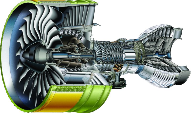
Trent 1000 Turbofan Engine. Source: Reproduced with permission from Rolls-Royce plc
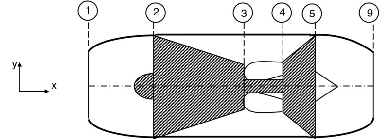
An aircraft engine is designed to produce thrust F (or sometimes lift in VTOL/STOL aircraft, e.g., the lift fan in the Joint Strike Fighter, F-35). In an airbreathing engine, a mass flow rate of air and fuel are responsible for creating that thrust. In a liquid rocket engine, the air is replaced with an onboard oxidizer , which then reacts with an onboard fuel to produce thrust. Although we will discuss the internal characteristics of a gas turbine engine in Chapter 4, it is instructive to show the station numbers in a two-spool turbojet engine with an afterburner. Figure 3.1 is schematic drawing of such engine. The air is brought in through the air intake, or inlet, system, where station 0 designates the unperturbed flight condition, station 1 is at the inlet (or cowl) lip, and station 2 is at the exit of the air intake system, which corresponds to the inlet of the compressor (or fan). The compression process from stations 2 to 3 is divided into a low-pressure compressor (LPC) spool and a high-pressure compressor (HPC) spool. The exit of the LPC is designated by station 2.5 and the exit of the HPC is station 3. The HPC is designed to operate at a higher shaft rotational speed than the LPC spool. The compressed gas enters the main or primary burner at 3 and is combusted with the fuel to produce hot high-pressure gas at 4 to enter the high-pressure turbine (HPT). Flow expansion through the HPT and the low-pressure turbine (LPT) produces the shaft power for the HPC and LPC, respectively. An afterburner is designated between stations 5 and 7, where an additional fuel is combusted with the turbine discharge flow before it expands in the exhaust nozzle. Station 8 is at the throat of the nozzle and station 9 designates the nozzle exit.
FIGURE 3.1Station numbers for an afterburning turbojet engine
To derive an expression for the engine thrust, it is most convenient to describe a control volume surrounding the engine and apply momentum principles to the fluid flow crossing the boundaries of the control volume. Let us first consider an airbreathing engine. From a variety of choices that we have in describing the control volume, we may choose one that shares the same exit plane as the engine nozzle, and its inlet is far removed from the engine inlet so not to be disturbed by the nacelle lip. These choices are made for convenience. As for the sides of the control volume, we may choose either stream surfaces, with the advantage of no flow crossing the sides, or a constant-area box, which has a simple geometry but fluid flow crosses the sides. Regardless of our choice of the control volume, however, the physical expression derived for the engine thrust has to produce the same force in either method. Figure 3.2 depicts a control volume in the shape of a box around the engine.
FIGURE 3.2Schematic drawing of an airbreathing engine with a box-like control volume positioned around the engine (Note the flow of air to the engine, through the sides, and the fuel flow rate)
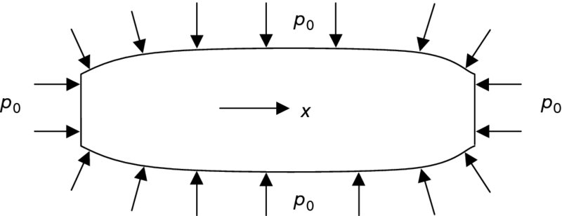
The pylon, by necessity, is cut by the control volume, which is enclosing the engine. The thrust force F and its reaction are shown in Figure 3.2. We may assume the sides of the control volume are not affected by the flowfield around the nacelle, that is, the static pressure distribution on the sides is nearly the same as the ambient static pressure p0. In the same spirit, we may assume that the exit plane also sees an ambient pressure of p0 with an exception of the plane of the jet exhaust, where a static pressure p9 may prevail. To help us balance momentum flux and net forces acting on the fluid crossing the control surface, we show the external pressure distributions as in Figure 3.3.
FIGURE 3.3Simplified model of static pressure distribution on the surface of the control volume
From our study of fluid mechanics, we know that the closed surface integral of a constant pressure results in a zero net force acting on the closed surface, that is,
(3.1)
where is the unit normal vector pointing out of the control surface, ds is the elemental surface area, and the negative sign shows that the direction of the pressure is in the inward normal direction to the closed surface. The equivalence of the closed surface integral and the volume integral via the gradient theorem may be used to prove the above principle, namely;
(3.2)
where dv is the element of volume and ∇p is the pressure gradient vector. Note that ∇p ≡ 0 for a constant p. Now, let us subtract the constant ambient pressure p0 from all sides of the closed surface of the control volume shown in Figure 3.4, to get a net pressure force acting on the control surface.
FIGURE 3.4Simplified model of the static pressure force acting on the control surface
As we are interested in deriving an expression for a force, namely thrust, we have to use the momentum conservation principles, namely, we need to balance the fluid momentum in the x-direction and the resultant external forces acting on the fluid in the x-direction. Before doing that, we must establish the fluid flow rates in and out of the control volume. This is achieved by applying the law of conservation of mass to the control volume. In its simplest form, that is, steady flow case, we have
Applying Equation 3.3 to the control volume surrounding our engine (Figure 3.5) gives the following bookkeeping expression on the mass flow rates in and out of the box, namely,
FIGURE 3.5Control volume and the mass flow rates in and out of its boundaries
Now, we are ready to apply the momentum balance to the fluid entering and leaving our control volume. Again assuming steady, uniform flow, we may use the simplest form of the momentum equation, that is,
which states that the difference between the fluid (time rate of change of) momentum out of the box and into the box is equal to the net forces acting on the fluid in the x-direction on the boundaries and within the box. Now, let us spell out each of the contributions to the momentum balance of Equation 3.6, that is,
Now, through the action–reaction principle of the Newtonian mechanics, we know that an equal and opposite axial force is exerted on the engine, by the fluid, that is,
(3.12)
Therefore, calling the axial force of the engine “thrust, ” or simply F, we get the following expression for the engine thrust
This expression for the thrust is referred to as the “net uninstalled thrust” and sometimes a subscript “n” is placed on F to signify the “net” thrust. Therefore, the thrust expression of Equation 3.13 is better written as
Now, we attribute a physical meaning to the three terms on the right-hand side (RHS) of Equation 3.14, which contribute to the engine net (uninstalled) thrust. We first note that the RHS of Equation 3.14 is composed of two momentum terms and one pressure–area term. The first momentum term is the exhaust momentum through the nozzle contributing positively to the engine thrust. The second momentum term is the inlet momentum, which contributes negatively to the engine thrust in effect it represents a drag term. This drag term is called “ram drag, ” or simply the penalty of bringing air in the engine with a finite momentum. It is often given the symbol of Dram and expressed as
The last term in Equation 3.14 is a pressure–area term, which acts over the nozzle exit plane, that is, area A9, and will contribute to the engine thrust only if there is an imbalance of static pressure between the ambient and the exhaust jet. As we remember from our aerodynamic studies, a nozzle with a subsonic jet will always expand the gases to the same static pressure as the ambient condition, and a sonic or supersonic exhaust jet may or may not have the same static pressure in its exit plane as the ambient static pressure. Depending on the “mismatch” of the static pressures, we categorized the nozzle flow as
Examining the various contributions from Equation 3.14 to the net engine (uninstalled) thrust, we note that the thrust is the difference between the nozzle contributions (both momentum and pressure–area terms) and the inlet contribution (the momentum term). The nozzle contribution to thrust is called gross thrust and is given a symbol Fg, that is,
(3.16)
and, as explained earlier, the inlet contribution was negative and was called “ram drag” Dram, therefore
Now, we can generalize the result expressed in Equation 3.17 to aircraft engines with more than a single stream, as, for example, the turbofan engine with separate exhausts. This task is very simple as we account for all gross thrusts produced by all the exhaust nozzles and subtract all the ram drag produced by all the air inlets to arrive at the engine uninstalled thrust, that is,
(3.18)
Another way of looking at this is to balance the momentum of the exhaust stream and the inlet momentum with the pressure thrust at the nozzle exit planes and the net uninstalled thrust of the engine. In a turbofan engine, the captured airflow is typically divided into a “core” flow, where the combustion takes place, and a fan flow, where the so-called “bypass” stream of air is compressed through a fan and later expelled through a fan exhaust nozzle. This type of arrangement, that is, bypass configuration, leads to a higher overall efficiency of the engine and lower fuel consumption. A schematic drawing of the engine is shown in Figure 3.6.
FIGURE 3.6Schematic drawing of a turbofan engine with separate exhausts
In this example, the inlet consists of a single (or dual) stream, and the exhaust streams are split into a primary and a fan nozzle. We may readily write the uninstalled thrust produced by the engine following the momentum principle, namely,
(3.19)
The first four terms account for the momentum and pressure thrusts of the two nozzles (what is known as gross thrust) and the last term represents the inlet ram drag.
3.1.1 Takeoff Thrust
At takeoff, the air speed V0 (“flight” speed) is often ignored in the thrust calculation, therefore the ram drag contribution to engine thrust is neglected, that is,
(3.20)
For a perfectly expanded nozzle, the pressure thrust term vanishes to give
Therefore, the takeoff thrust is proportional to the captured airflow.
3.2 Installed Thrust—Some Bookkeeping Issues on Thrust and Drag
As indicated by the description of the terms “installed thrust” and “uninstalled thrust, ” they refer to the actual propulsive force transmitted to the aircraft by the engine and the thrust produced by the engine if it had zero external losses, respectively. Therefore, for the installed thrust, we need to account for the installation losses to the thrust such as the nacelle skin friction and pressure drags that are to be included in the propulsion side of the drag bookkeeping. On the contrary, the pylon and the engine installation that affects the wing aerodynamics (in podded nacelle, wing-mounted configurations), namely by altering its “clean” drag polar characteristics, causes an “interference” drag that is accounted for in the aircraft drag polar. In the study of propulsion, we often concentrate on the engine “internal” performance, that is, the uninstalled characteristics, rather than the installed performance because the external drag of the engine installation depends not only on the engine nacelle geometry but also on the engine–airframe integration. Therefore, accurate installation drag accounting will require computational fluid dynamics (CFD) analysis and wind tunnel testing at various flight Mach numbers and engine throttle settings. In its simplest form, we can relate the installed and uninstalled thrust according to
(3.22)
In our choice of the control volume as depicted in Figure 3.2, we made certain assumptions about the exit boundary condition imposed on the aft surface of the control volume. We made assumptions about the pressure boundary condition as well as the velocity boundary condition. About the pressure boundary condition, we stipulated that the static pressure of flight p0 imposed on the exit plane, except at the nozzle exit area of A9, therefore we allowed for an under- or overexpanded nozzle. With regard to the velocity boundary condition at the exit plane, we stipulated that the flight velocity V0 prevailed, except at the nozzle exit where the jet velocity of V9 prevails. In reality, the aft surface of the control volume is, by necessity, downstream of the nacelle and pylon, and therefore it is in the middle of the wake generated by the nacelle and the pylon. This implies that there would be a momentum deficit in the wake and the static pressure nearly equals the free stream pressure. The velocity profile in the exit plane, that is, the wake of the nacelle and pylon, is more likely to be represented by the schematic drawing in Figure 3.7.
FIGURE 3.7Velocity profile in the nacelle and pylon wake showing a momentum deficit region
However, the force transmitted through the pylon to the aircraft is not the “uninstalled” thrust, as we called it in our earlier derivation, rather the installed thrust and pylon drag. But the integral of momentum deficit and the pressure imbalance in the wake is exactly equal to the nacelle and pylon drag contributions, that is, we have
(3.23)
where the surface integral is taken over the exit plane downstream of the nacelle and pylon.
Now, let us go back and correct for the wake contributions noted in Equation 3.21 as well as the actual force transmitted through the pylon, namely,
After canceling the integrals on the RHS with the drag terms of the left-hand side (LHS) in Equation 3.24, we recover Equation 3.14 that we derived earlier for the uninstalled thrust, that is
As noted earlier, we are not limited to the choice of the control volume that we made in the form of a box wrapped around the engine and cutting through the pylon (Figure 3.2). Let us examine other logical choices that we could have made. For example, we could use the inlet-captured streamtube as the upstream portion of the control volume and allow the nacelle external surface to serve as the remaining portion of the control volume, and then truncate the control volume at the nozzle exit plane. This choice of control volume is schematically shown in Figure 3.8.
FIGURE 3.8Schematic drawing of an alternative control volume
The choice of the control volume depicted in Figure 3.8 offers the advantage of no airflow crossing the sides of the control surface. There is, of course, the fuel flow rate through the pylon and the airflow rates through the inlet-captured streamtube (station 0) and the nozzle exit plane (station 9), as expected. The penalty of using this control volume is in the more complicated force balance terms, which appear in the momentum equation. The pressure distribution on the captured streamtube, for example, will correspond to a diffusing stream pattern, from station 0 to 1, therefore, the static pressure increases along the captured streamtube. Then, the static pressure is decreased to the point of maximum nacelle diameter (station labeled M) as the flow accelerates from the inlet lip stagnation point. From the position of minimum static pressure at M, the flow is diffused on the aft end of the nacelle and will recover most of the static pressure and almost reach the flight ambient pressure p0. The static pressure distribution on the control surface is schematically shown in Figure 3.9.
FIGURE 3.9Sketch of the static pressure distribution on the sides of the control surface, including the capture streamtube and the nacelle
Following Newton’s second law of motion, we stipulate that the change of momentum of fluid crossing the boundaries of the control volume (Figure 3.8) in the x-direction, say, is balanced by the net forces acting on the fluid in the x-direction. Therefore,
where the LHS is the net gain in x-momentum, which is created by the net forces in the positive x-direction acting on the fluid, that is, the RHS terms of Equation 3.25.
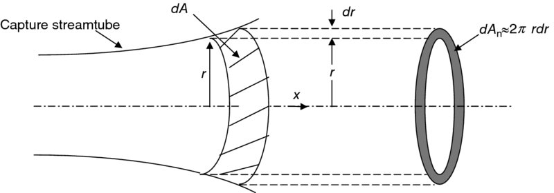
The external forces are due to pressure and frictional stresses acting on the control surface in the x-direction. In the x-balance of momentum, the reader notes that the gravitational force does not enter the calculation at any case and in general we do not include the effect of gravitational force, as it represents a negligible contribution to the force balance involving aircraft jet propulsion. Now, let us breakdown the elements of external force, which act on the control surface. First, the pressure integral over the captured streamtube acting on the fluid in the x-direction can be written
where the element of area dAn is the change of the area of the captured streamtube normal to the x-direction, that is, varying from A0 at the inlet to A1 at the exit, therefore experiencing (A1 − A0) change over the length of the captured streamtube. We can use the Figure 3.10 as an aid in demonstrating what is meant by dAn.
FIGURE 3.10Definition sketch for dA and its projection normal to the x-axis dAn
On the captured streamtube depicted in Figure 3.8 (or 3.9), the local pressure p is greater than the ambient pressure p0, and dAn is also positive, as the captured streamtube widens (dA > 0), hence the pressure integral of Equation 3.26 is positive. This means that the flow deceleration outside the inlet will contribute a positive force in the x-direction on the control surface, which represents a drag for the engine installation. This drag term is called pre-entry drag or additive drag. It is interesting to note that if the captured streamtube were inverted, that is, it caused external flow acceleration instead of deceleration, a typical scenario for takeoff and climb or the engine static testing, then the local static pressure would drop below ambient pressure, which causes the integrand (p − p0) to be negative. Despite this, we still encounter a pre-entry drag, as we note that dAn is also negative for a shrinking streamtube, hence the pre-entry momentum contribution remains as a penalty, that is, a drag term. This is schematically shown in Figure 3.11.
where the element of area is again represented by the change of area normal to the x-direction. The integral of pressure over the inlet cowl (i.e., from 1 to M) represents a thrust contribution, as the wall static pressure on the forward region of the cowl is below the ambient pressure, that is, p − p0 < 0, and dAn is positive, therefore the pressure integral of Equation 3.27 is negative. A negative force in the x-direction represents a thrust term. This force may be thought of as the suction force on a circular wing (to represent the inlet cowl lip) projected in the x-direction. To demonstrate this point, we examine the following schematic drawing (Figure 3.12).
FIGURE 3.12Flow detail near a blunt cowl lip showing a lip thrust component and a side force
For an axisymmetric inlet, the aerodynamic side force created on the nacelle integrates to zero, but as most engine nacelles are asymmetrical for either ground clearance or accessibility of the engine accessories reasons, a net side force is created on the nacelle, as well.
The inlet additive drag is thus for the most part balanced by the cowl lip thrust and the difference is called the spillage drag, that is,
(3.28)
In general, for well-rounded cowl lips of subsonic inlets, the spillage drag is rather small and it becomes significant for only supersonic, sharp-lipped inlets. The nacelle frictional drag also contributes to the external force as well as the aft-end pressure drag of the boattail, which may be written as
(3.29)
The first term on the RHS, that is, (I), is the spillage drag that we discussed earlier, the second term (II) is the pressure drag on the nacelle aft end or boat tail pressure drag, the third term (III) is the nacelle viscous drag, the fourth term (IV) is the pylon drag, the fifth term (V) is the reaction to the installed thrust force and pylon drag acting on the fluid, and the last term (VI) is the pressure thrust due to imperfect nozzle expansion. To summarize
Terms I + II + III are propulsion system installation drag losses
Term IV is accounted for in the aircraft drag polar
Terms V and VI combine with I, II, III, and IV to produce the uninstalled thrust.
Therefore, we recover the expression for the uninstalled thrust that we had derived using another control volume for an airbreathing engine, namely
Figure 3.13 shows the elements of force that contribute to installed net thrust.
FIGURE 3.13Definition of installed net thrust in terms of internal and external parameters of an engine nacelle (adapted from Lotter, 1977)
3.3 Engine Thrust Based on the Sum of Component Impulse
We have derived an expression for a component internal force based on the fluid impulse at its inlet and exit in Chapter 2. We wish to demonstrate the relationship between the sum of the component forces and the engine thrust.
The axial component of force felt by the inner walls of the diffuser (from 1 to 2), see Figure 3.14, is
(3.30)
FIGURE 3.14Definition sketch used in engine thrust calculation based on component impulse
The axial component force felt by the inner walls of the compressor (from 2 to 3) is
(3.31)
The axial component force felt by the inner walls of the combustor (from 3 to 4) is
(3.32)
The axial component force felt by the inner walls of the turbine (from 4 to 5) is
(3.33)
The axial component force felt by the inner walls of the nozzle (from 5 to 9) is
Therefore, the total internal axial force acting on the inner walls of the engine is
(3.35)
The thrust acts in the −x-direction, therefore the engine internal thrust is (minus the above)
(3.36)
However, in flight we neither know V1 nor p1. To connect the inlet flow to the flight condition, we examine the captured streamtube, as shown in Figure 3.15.
FIGURE 3.15Pressure distribution on the captured streamtube
We have subtracted a constant pressure p0 from all sides, as shown in Figure 3.15. The momentum balance in the x-direction gives
(3.37)
The integral on the RHS is called the additive drag Dadd, therefore,
(3.38)
(3.39)
The integral of constant pressure distribution p0 around the nacelle, as in Figure 3.16, leads to
(3.40)
FIGURE 3.16Nacelle under a constant pressure distribution
Therefore, we may replace p0A1 by p0A9 and the integral on the sides to get
(3.41)
The external forces acting on the nacelle (in the x-direction) arise from pressure and shear integrals, namely
(3.42)
The integral of pressure on the nacelle lip produces a lip thrust force, which almost cancels the inlet additive drag (Figure 3.17), that is,
(3.43)
FIGURE 3.17Nacelle lip pressure distribution and the resulting force
Therefore, the net installed thrust, after canceling inlet additive drag with the lip suction force, is
(3.44)
The uninstalled thrust thus connects the free stream to the nozzle exit, after we account for the additive drag and the nacelle lip suction force to cancel each other. The leftover external pressure and shear integral are then attributed to installation drag.
(3.45)
3.4 Rocket Thrust
Although our primary effort in this book is to study airbreathing propulsion, the subject of rocket propulsion has been presented in Chapter 12. For now, we may think of the rocket thrust as a special case of an airbreathing engine with a “sealed inlet” ! It is simply too tempting to ignore this special case of jet propulsion with no inlet penalty. Figure 3.18 shows a schematic drawing of a rocket engine where all the propellant, that is, fuel and oxidizer, is stored in specialized tanks onboard the rocket.
FIGURE 3.18Schematic drawing of liquid propellant rocket engine internal components
The thrust produced by a rocket engine amounts to only the gross thrust produced by an airbreathing engine. We remember that the gross thrust was the nozzle contribution to thrust, which a rocket also possesses to accelerate the combustion gas. The air intake system is missing in a rocket, and therefore the inlet ram drag contribution is also absent from the rocket thrust equation. Consequently, we can express the rocket thrust as
It is interesting to note that the rocket thrust is independent of flight speed V0, as Equation 3.46 does not explicitly involve V0. However, if the flight trajectory has a vertical component to it, then the ambient pressure p0 changes with altitude, and therefore the pressure thrust term of Equation 3.46 will then affect the thrust magnitude. For example, the space shuttle main engine produces about 25% more thrust in “vacuum” than at sea level, mainly due to the pressure thrust difference between sea level p0 of 14.7 psia (or 1 atm) and p0 of zero corresponding to “vacuum” in near earth orbit.
Again, for the net propulsive force acting on the rocket, we need to account for the vehicle external drag. Although, the Equation 3.46 is not explicitly referred to as “uninstalled” thrust in rocket propulsion literature, the reader should view it as the internal performance of a rocket engine. The external aerodynamic analysis will produce control forces and vehicle external drag contributions.
3.5 Airbreathing Engine Performance Parameters
The engine thrust, mass flow rates of air and fuel, the rate of kinetic energy production across the engine or the mechanical power/shaft output, and engine dry weight, among other parameters, are combined to form a series of important performance parameters, known as the propulsion system figures of merit.
3.5.1 Specific Thrust
The size of the air intake system is a design parameter that establishes the flow rate of air, . Accordingly, the fuel pump is responsible for setting the fuel flow rate in the engine, . Therefore, in producing thrust in a “macroengine, ” the engine size seems to be a “scaleable” parameter. The only exception in scaling the jet engines is the “microengines” where the component losses do not scale. In general, the magnitude of the thrust produced is directly proportional to the mass flow rates of the fluid flow through the engine. Then, it is logical to study thrust per unit mass flow rate as a figure of merit of a candidate propulsion system. In case of an airbreathing engine, the ratio of thrust to air mass flow rate is called specific thrust and is considered to be an engine performance parameter, that is,
The target for this parameter, that is, specific thrust, in a cycle analysis is usually to be maximized, that is, to produce thrust with the least quantity of air flow rate, or equivalently to produce thrust with a minimum of engine frontal area. However, with subsonic cruise Mach numbers, the drag penalty for engine frontal area is far less severe than their counterparts in supersonic flight. Consequently, the specific thrust as a figure of merit in a commercial transport aircraft (e.g., Boeing 777 or Airbus A-340) takes a back seat to the lower fuel consumption achieved in a very large bypass ratio turbofan engine at subsonic speeds. As noted, specific thrust is a dimensional quantity with the unit of force per unit mass flow rate. A nondimensional form of the specific thrust, which is useful for graphing purposes and engine comparisons, is (following Kerre-brock, 1992)
(3.47)
where a0 is the ambient speed of sound taken as the reference velocity.
3.5.2 Specific Fuel Consumption and Specific Impulse
The ability to produce thrust with a minimum of fuel expenditure is another parameter that is considered to be a performance parameter in an engine. In the commercial world, for example, the airline business, specific fuel consumption represents perhaps the most important parameter of the engine. After all, the money spent on fuel is a major expenditure in operating an airline, for example. However, the reader is quickly reminded of the unspoken parameters of reliability and maintainability that have a direct impact on the cost of operating commercial engines and, therefore, they are at least as important, if not more important, as the engine-specific fuel consumption. In the military world, the engine fuel consumption parameter takes a decidedly secondary role to other aircraft performance parameters, such as stealth, agility, maneuverability, and survivability. For an airbreathing engine, the ratio of fuel flow rate per unit thrust force produced is called thrust-specific fuel consumption (TSFC), or sometimes just the specific fuel consumption (sfc) and is defined as
The target for this parameter, that is, TSFC, in a cycle analysis is to be minimized, that is, to produce thrust with a minimum of fuel expenditure. This parameter, too, is dimensional. For a rocket, on the contrary, the oxidizer as well as the fuel both contribute to the “expenditure” in the engine to produce thrust, and as such the oxidizer flow rate needs to be accounted for as well. The word “propellant” is used to reflect the combination of oxidizer and fuel in a liquid propellant rocket engine or a solid propellant rocket motor. It is customary to define a corresponding performance parameter in a rocket as thrust per unit propellant weight flow rate. This parameter is called specific impulse Is, that is,
and g0 is the gravitational acceleration on the surface of the earth, that is 9.8 m/s2 or 32.2 ft/s2. The dimension of in the denominator of Equation 3.48 is then the weight flow rate of the propellant based on earth’s gravity, or force per unit time. Consequently, the dimension of specific impulse is “Force/Force/second” which simplifies to just the “second.” All propulsors, rockets, and airbreathers, then could be compared using a unifying figure of merit, namely their specific impulse in seconds. An added benefit of the specific impulse is that regardless of the units of measurement used in the analysis, that is, either metric or the British on both sides of the Atlantic, specific impulse comes out as seconds in both systems. The use of specific impulse as a unifying figure of merit is further justified in the twenty-first century as we attempt to commercialize space with potentially reusable rocket-based combined cycle (RBCC) power plants in propelling a variety of single-stage-to-orbit (SSTO) vehicles. To study advanced propulsion concepts where the mission calls for multimode propulsion units, as in air-ducted rockets, ramjets, and scramjets, all combined into a single “package, ” the use of specific impulse becomes even more obvious. In summary,
An important goal in an engine cycle design is to maximize this parameter, that is, the ability to produce thrust with the least amount of fuel or propellant consumption in the engine.
3.5.3 Thermal Efficiency
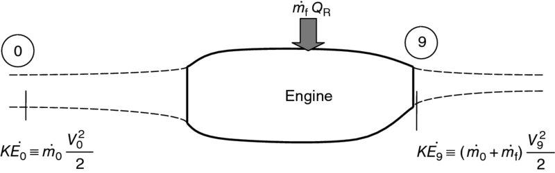
The ability of an engine to convert the thermal energy inherent in the fuel (which is unleashed in a chemical reaction) to a net kinetic energy gain of the working medium is called the engine thermal efficiency, ηth. Symbolically, thermal efficiency is expressed as
where signifies mass flow rate corresponding to stations 0 and 9, subscript “f” signifies fuel, and QR is the fuel heating value. The unit of QR is energy per unit mass of the fuel (e.g., kJ/kg or BTU/lbm) and is tabulated as a fuel property. Equation 3.50 compares the mechanical power production in the engine to the thermal power investment in the engine. Figure 3.19 is a definition sketch, which is a useful tool to help remember thermal efficiency definition, as it graphically depicts the energy sources in an airbreathing engine. The rate of thermal energy consumption in the engine and the rate of mechanical power production by the engine are not equal. Yet, we are not violating the law of conservation of energy. The thermal energy production in an engine is not actually “lost, ” as it shows up in the hot jet exhaust stream, rather this energy is “wasted” and we were unable to convert it to a “useful” power. It is important to know, that is, to quantify, this inefficiency in our engine.
FIGURE 3.19Thermal power input and the mechanical power production (output)
Equation 3.50, which defines thermal efficiency, is simply the ratio of “net mechanical output” to the “thermal input, ” as we had learned in thermodynamics.
Example 3.4 shows a turbojet engine (with the specified parameters) is only about 49.2% thermally efficient! What happened to the rest of the fuel (thermal) energy? We know that ∼49.2% of it was converted to a net mechanical output and the remaining 51.8% then must have been untapped and left in the exhaust gas as thermal energy. The thermal energy in the exhaust gas is of no use to the vehicle and, in fact, in many applications, costs an additional weight that needs to be considered for cooling/thermal protection of the exhaust nozzle and nearby structures. The thermal energy in the exhaust gas of an aircraft engine basically goes to waste. Therefore, the lower the exhaust gas temperature, the more useful energy is extracted from the combustion gases and, hence, the cycle is more efficient in the thermal context. Now, you may wonder what other context is there, besides the thermal efficiency context in a heat engine? The answer is found in the application of the engine. The purpose of an aircraft engine is to provide propulsive power to the aircraft. In simple terms, the engine has to produce a thrust force that can accelerate the vehicle to a desired speed, for example, from takeoff to cruise condition, or maintain the vehicle speed, that is, just to overcome vehicle drag in cruise. Of course, one may add the hover and lifting applications to an aircraft engine purpose as, for example, in helicopters and short takeoff and landing (STOL) aircraft, respectively. Therefore, there is another context other than the thermal efficiency for an aircraft engine, namely the propulsive efficiency. Before leaving our treatment of the thermal efficiency of the jet engines and investigating their propulsive efficiency, let us explore various ways of improving the thermal efficiency for an aircraft engine.
To lower the exhaust gas temperature, we can place an additional turbine wheel in the high pressure, hot gas stream and produce shaft power. This shaft power can then be used to power a propeller, a fan, or a helicopter rotor, for example. The concept of additional turbine stages to extract thermal energy from the combustion gases and powering a fan in a jet engine has led to the development of more efficient two- or three-spool turbofan engines. Therefore, the mechanical output of these engines is enhanced by the additional shaft power. The thermal efficiency of a cycle that produces a shaft power can therefore be written as
(3.51)
A schematic drawing of an aircraft gas turbine engine, which is configured to produce shaft power, is shown in Figure 3.20. In Figure 3.20a, the “power turbine” provides shaft power to a propeller, whereas in Figure 3.20b, the power turbine provides the shaft power to a helicopter main rotor.
FIGURE 3.20Schematic drawing of a power turbine placed in the exhaust of a gas turbine engine
The gas generator in Figure 3.20 refers to the compressor, burner, and the turbine combination, which are detailed in the next chapter. In turboprops and turboshaft engines, the mechanical output of the engine is dominated by the shaft power; therefore, in the definition of the thermal efficiency of such cycles the rate of kinetic energy increase is neglected, that is,
(3.52)
In addition to a shaft-power turbine concept, we can lower the exhaust gas temperatures by placing a heat exchanger in the exhaust stream to preheat the compressor air prior to combustion. The exhaust gas stream is cooled as it heats the cooler compressor gas and the less fuel need be burnt to achieve a desired turbine entry temperature. This scheme is referred to as regenerative cycle and is shown in Figure 3.21.
FIGURE 3.21Schematic drawing of a gas turbine engine with a regenerative scheme
All of the cycles shown in Figures 3.20 and 3.21 produce less wasted heat in the exhaust nozzle; consequently, they achieve a higher thermal efficiency than their counterparts without the extra shaft power or the heat exchanger. However, we engineers need to examine a bottom line question all the time, that is, “will our gains outweigh our losses?” Obviously we gain in thermal efficiency but our systems in all instances require more complexity and weight. System complexity ties in with the issues of reliability and maintenance and the system weight ties in with the added cost and thus market acceptability. Therefore, we note that a successful engine does not necessarily have the highest thermal efficiency, but rather its overall system performance and cost is designed to meet the customer’s requirements in an optimum manner. And in fact, its thermal efficiency is definitely compromised by the engine designers within the propulsion system design optimization loop/process. We will return to the issues surrounding thermal efficiency in every cycle we study in the next chapter.
Finally, one last question before we leave this subject is that “is it possible to achieve a 100% thermal efficiency in an aircraft engine?” This was actually a trick question to see who remembered his/her thermo! The answer is obviously no! We cannot violate the second law of thermodynamics. We remember that the highest thermal efficiency attainable in a heat engine operating between two temperature limits was that of a Carnot cycle operating between those temperatures. Figure 3.22 shows the Carnot cycle on a T–s diagram.
As noted in Figure 3.22, both heat rejection at absolute zero (T1 = 0) and heating to infinite temperatures (T2 = ∞) are impossibilities, therefore we are thermodynamically bound by the Carnot thermal efficiency as the maximum (<100%). A Brayton cycle, which gas turbine engines are represented by, experiences a lower thermal efficiency than the Carnot cycle and this subject is presented in the cycle analysis (Chapter 4) in more detail.
3.5.4 Propulsive Efficiency
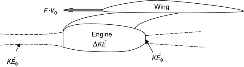
The fraction of the net mechanical output of the engine which is converted into thrust power is called the propulsive efficiency. The net mechanical output of the engine is for perfectly expanded nozzle and the thrust power is F · V0, therefore, the propulsive efficiency is defined as their ratio:
A graphical depiction of propulsive efficiency is shown in Figure 3.23 to help the reader to remember the definition of propulsive efficiency.
FIGURE 3.23Schematic drawing of an engine installation showing the mechanical and thrust power
Although the thrust power represented by F · V0 in Equation 3.53 is based on the installed thrust, for simplicity, it is often taken as the uninstalled thrust power to highlight a very important, and at first astonishing, result about the propulsive efficiency. Now, let us substitute the uninstalled thrust of a perfectly expanded jet in the above definition to get
We recognize that the fuel flow rate is but a small fraction (∼ 2%) of the air flow rate and thus can be ignored relative to the air flow rate; thus Equation 3.54 can be simplified to
Equation 3.55 as an approximate expression for the propulsive efficiency of a jet engine is cast in terms of a single parameter, namely the jet-to-flight velocity ratio V9 / V0. We further note that 100% propulsive efficiency (within the context of approximation presented in the derivation) is mathematically possible and will be achieved by engines whose exhaust velocity is as fast as the flight velocity, that is, V9 = V0. But a practical question poses itself, “how can we produce thrust in an airbreathing jet engine if the jet velocity is not faster than the flight velocity?” The short answer is that we cannot! Therefore, we conclude that some overspeeding in the jet, compared with flight speed, is definitely needed to produce reaction thrust in an airbreathing jet engine. Therefore for practical reasons, a 100% propulsive efficiency is not possible, just as the thermal efficiency of 100% was not possible. However, the smaller the increment of velocity rises across the engine, the higher its propulsive efficiency will be. In order to achieve a small velocity increment across a gas turbine engine for a given fuel flow rate, we need to drain the thermal energy in the combustion gas further and convert it to additional shaft power that in turn can act on a larger mass flow rate of air, in a secondary or a bypass stream, for example, a fan or a propeller, to produce the desired level of thrust.
FIGURE 3.24Schematic drawing of a turbojet engine in flight with a velocity ratio of 4.5
FIGURE 3.25Schematic drawing of a turbofan engine in flight with a velocity ratio of 1.25
Propulsive efficiency of a turboprop engine is defined as the fraction of mechanical power that is converted to the total thrust (i.e., the sum of propeller and engine nozzle thrust) power, namely
Again, this definition compares the propulsive output(F · V0) to the mechanical power input (shaft and jet kinetic energy change) in an aircraft engine. The fraction of shaft power delivered to the propeller that is converted to the propeller thrust is called propeller efficiencyηprop
(3.57)
Due to large diameters of propellers, it is necessary to reduce their rotational speed to avoid severe tip shock-induced losses. Consequently, the power turbine rotational speed is mechanically reduced in a reduction gearbox and a small fraction of shaft power is lost in the gearbox, which is referred to as gear box efficiency, that is,
(3.58)
We will address turboprop performance in Chapter 4.
3.5.5 Engine Overall Efficiency and Its Impact on Aircraft Range and Endurance
The product of the engine thermal and propulsive efficiency is called the engine overall efficiency
(3.59)
The overall efficiency of an aircraft engine is therefore the fraction of the fuel thermal power that is converted into the thrust power of the aircraft. Again a useful output is compared with the input investment in this efficiency definition. In an aircraft performance course that typically precedes the aircraft propulsion class, the engine overall efficiency is tied with the aircraft range through the Breguet range equation. The derivation of the Breguet range equation is both fundamental to our studies and surprisingly simple enough for us to repeat it here for review purposes. An aircraft in level flight cruising at the speed of V0 (Figure 3.26) experiences a drag force that is entirely balanced by the engine thrust (for no acceleration), that is,
FIGURE 3.26Aircraft in an un-accelerated level flight
FIGURE 3.27V2500 engine cutaway. Source: Reproduced by permission of United Technologies Corporation, Pratt & Whitney
FIGURE 3.28PW6000 engine cutaway. Source: Reproduced by permission of United Technologies Corporation, Pratt & Whitney
FIGURE 3.29The PW1000G engine. Source: Reproduced by permission of United Technologies Corporation, Pratt & Whitney
FIGURE 3.30The PW4000 112-inch fan engine. Source: Reproduced by permission of United Technologies Corporation, Pratt & Whitney
FIGURE 3.31GP7000 engine cutaway. Source: Reproduced by permission of United Technologies Corporation, Pratt & Whitney
FIGURE 3.32F135 engine cutaway: (a) conventional takeoff and landing; (b) short takeoff, vertical landing. Source: Reproduced by permission of United Technologies Corporation, Pratt & Whitney
FIGURE 3.33F119 engine cutaway. Source: Reproduced by permission of United Technologies Corporation, Pratt & Whitney
The aircraft lift L is also balanced by the aircraft weight to maintain level flight, that is,
(3.61)
We can multiply Equation 3.60 by the flight speed V0 and then replace the resulting thrust power, F·V0, by , via the definition of the engine overall efficiency, to get
Noting that the fuel flow rate, , that is, the rate at which the aircraft is losing mass (thus the negative sign), we can substitute this expression in Equation 3.63 and rearrange to get
where g0 is the Earth’s gravitational acceleration and V0dt is interpreted as the aircraft elemental range dR, which is the distance traveled in time dt by the aircraft at speed V0. Now, we can proceed to integrate Equation 3.64 by making the assumptions of constant lift-to-drag ratio and constant engine overall efficiency, over the cruise period, to derive the Breguet range equation as
where Wi is the aircraft initial weight and Wf is the aircraft final weight (note that the initial weight is larger than the final weight by the weight of the fuel burned in flight). Equation 3.65 is known as the Breguet range equation, which owes its simplicity and elegance to our assumptions of (1) unaccelerated level flight and (2) constant lift-to-drag ratio and engine overall efficiency. Also note that the range segment contributed by the takeoff, climb and approach and landing distances is not accounted for in the Breguet range equation. The direct proportionality of the engine overall efficiency and the aircraft range is demonstrated by the Breguet range equation, that is,
Now, let us replace the overall efficiency of the engine in the range equation by the ratio of thrust power to the thermal power in the fuel according to
(3.66)
We may express the flight speed in terms of a product of flight Mach number and the speed of sound; in addition, we may substitute the thrust specific fuel consumption for the ratio of fuel flow rate to the engine net thrust, to get
The result of this representation of the aircraft range is the emergence of (ML/D) as the aerodynamic figure of merit for aircraft range optimization, known as the range factor,
(3.68)
(3.69)
Now, if we use a more energetic fuel than the current jet aviation fuel, for example hydrogen, we will be able to reduce the thrust specific fuel consumption, or we can see the effect of fuel energy content on the range following Equation 3.65, which shows
(3.70)
Equivalently, we may seek out the effect of engine overall efficiency, or the specific fuel consumption on aircraft endurance, which for our purposes is the ratio of aircraft range to the flight speed,
(3.71)
This again points out the importance of engine overall efficiency on aircraft performance parameters such as endurance. Now, let us substitute for engine overall efficiency and recast this equation in terms of TSFC, to get
(3.72)
The engine thrust-specific-fuel consumption appears in the denominator as in the engine impact on the range equation, and this time the aerodynamic figure of merit is L/D, instead of ML/D, as expected for the aircraft endurance.
(3.73)
(3.74)
For additional reading on the subject, Anderson (1999), Newman (2002) and Pratt & Whitney operations manual 200 (1988) are recommended.
3.6 Modern Engines, Their Architecture and Some Performance Characteristics
At the time of this writing, the science/engineering community is facing very strict compliance requirements in the United States on ITAR (International Traffic in Arms Regulation). This limits the availability of some engine performance parameters and data. With gratitude, I acknowledge the receipt of modern engine cutaways (Figures 3.27 to 3.33) and a table of engine data (Table 3.1) from United Technology Corporation, Pratt & Whitney. These are reproduced here with permission. The students in propulsion shall enjoy every single frame and data.
Source: Reproduced by permission of United Technologies Corporation, Pratt & Whitney.
3.7 Summary
In this chapter, we defined engine thrust and the factors outside the engine that influenced its “installed” performance. We noted that the specific fuel consumption is a “fuel economy” parameter and is thus very critical to the direct operating expenses of an aircraft. We also used component impulse formulation to demonstrate the thrust equation for an airbreathing engine. Thermal and propulsive efficiencies each measured the internal performance and thrust production efficiency of an engine in flight, respectively. The overall efficiency of the engine, as the product of thermal and propulsive efficiencies, is tied to both the fuel economy as well as aircraft range. A unifying figure of merit for airbreathing engines and rockets is “specific impulse” with units of seconds.
Airbreathing engines incur ram drag, which is the product of air mass flow rate and the flight speed. The exhaust nozzle produces gross thrust, which is the sum of the momentum thrust and a pressure force contribution that occurs for a nozzle with imperfect expansion. The gross thrust is maximized for a perfectly expanded nozzle where p9= p0. The sum of the gross thrust and the ram drag is the engine uninstalled thrust. The installation effects are primarily due to inlet and nacelle aft-end drag contributions.
Propulsive efficiency improves when the exhaust and flight speeds are closer to each other in magnitude, as in a turbofan engine. The parameter that brings the exhaust and flight speeds closer to each other in a turbofan engine is the bypass ratio. The trend in subsonic engine development/manufacturing is in developing ultra-high bypass (UHB) engines, with bypass ratio in 12–15 range. Pratt & Whitney has developed a geared UHB Turbofan engine, PW1000G, that represents the future of commercial aviation (shown in Section 3.6). Current conventional turbofan engines offer a bypass ratio of ∼8. Since the turboprop affects a much larger airflow at an incrementally smaller speed increase, it offers the highest propulsive efficiency for a low-speed (i.e., subsonic) aircraft. Advanced turboprops may utilize counterrotating propellers and may include a slimline nacelle, as in a ducted fan configuration.
Thermal efficiency is a cycle-dependent parameter. The highest thermal efficiency of a heat engine operating between two temperature limits corresponds to the Carnot cycle. Consequently, a higher compression (Brayton) cycle, still bound by two temperature limits, offers a higher thermal efficiency. The trend in improving engine thermal efficiency is in developing high-pressure ratio compressors. The current maximum (compressor pressure ratio in aircraft gas turbine engines) is ∼ 45–50.
References
Anderson, J.D., A, Aircraft Performance and Design, McGraw-Hill, New York, 1999.
Kerrebrock, J.L., Aircraft Engines and Gas Turbines, 2nd edition, MIT Press, Cambridge, Massachusetts, 1992.
Lotter, K., “Aerodynamische Probleme der Integration von Triebwerk und Zelle beim Kampfflugzeugen, ” Proceedings of the 85th Wehrtechnischen Symposium, Mannheim, Germany, 1977.
Newman, D., Interactive Aerospace Engineering and Design, McGraw-Hill, New York, 2002.
Pratt & Whitney Aircraft Gas Turbine Engine and Its Operation, P&W Operations Manual 200, 1988.
Problems
3.1 The total pressures and temperatures of the gas in an afterburning turbojet engine are shown (J57 “B” from Pratt & Whitney, 1988). The mass flow rates for the air and fuel are also indicated at two engine settings, the Maximum Power and the Military Power. Use the numbers specified in this engine to calculate
the fuel-to-air ratio f in the primary burner and the afterburner, at both power settings
the low- and high-pressure spool compressor pressure ratios and the turbine pressure ratio (note that these remain constant with the two power settings)
the exhaust velocity V9 for both power settings by assuming the specified thrust is based on the nozzle gross thrust (because of sea level static) and neglecting any pressure thrust at the nozzle exit
the thermal efficiency of this engine for both power settings (at the sea level static operation), assuming the fuel heating value is 18, 600 BTU/lbm and cp = 0.24 BTU/lbm · °R. Explain the lower thermal efficiency of the Maximum power setting
the thrust specific fuel consumption in lbm/h/lbf in both power settings
the Carnot efficiency of a corresponding engine, i.e., operating at the same temperature limits, in both settings
the comparison of percent thrust increase to percent fuel flow rate increase when we turn the afterburner on
why don’t we get proportional thrust increase with fuel flow increase (when it is introduced in the afterburner), i.e., doubling the fuel flow in the engine (through afterburner use) does not double the thrust
FIGURE P3.1Source: Reproduced by permission of United Technologies Corporation, Pratt & Whitney
3.2 The total pressures and temperatures of the gas are specified for a turbofan engine with separate exhaust streams (JT3D-3B from Pratt & Whitney, 1974). The mass flow rates in the engine core (or primary) and the engine fan are also specified for the sea level static operation. Calculate
the engine bypass ratio α defined as the ratio of fan-to-core flow rate
from the total temperature rise across the burner, estimate the fuel-to-air ratio and the fuel flow rate in lbm/h, assuming the fuel heating value is QR ∼ 18, 600 BTU/ lbm and the specific heat at constant pressure is 0.24 and 0.26 BTU/lbm · °R at the entrance and exit of the burner, respectively
the engine static thrust based on the exhaust velocities and the mass flow rates assuming perfectly expanded nozzles and compare your answer to the specified thrust of 18, 000 lbs
the engine thermal efficiency ηth
the thermal efficiency of this engine compared to the afterburning turbojet of Problem 1. Explain the major contributors to the differences in ηth in these two engines
the engine thrust specific fuel consumption in lbm/h/lbf
the nondimensional engine specific thrust
the Carnot efficiency corresponding to this engine
the engine overall pressure ratio pt3 / pt2
fan nozzle exit Mach number [use Tt = T + V2/2cp to calculate local static temperature at the nozzle exit, then local speed of sound a =(γRT)1/2]
FIGURE P3.2Source: Reproduced by permission of United Technologies Corporation, Pratt & Whitney
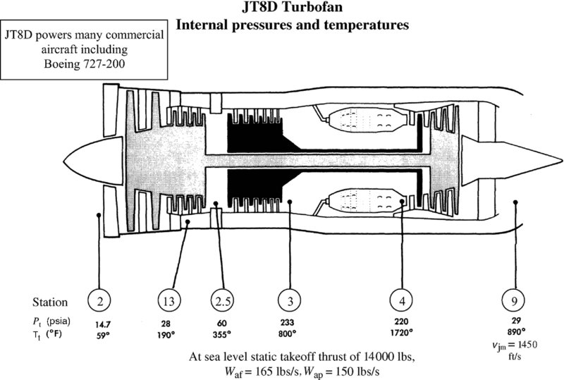
3.3 A mixed exhaust turbofan engine (JT8D from Pratt and Whitney, 1974) is described by its internal pressures and temperature, as well as air mass flow rates and the mixed jet (exhaust) velocity. Let us examine a few parameters for this engine, for a ballpark approximation.
Estimate the fuel flow rate from the total temperature rise across the burner assuming the fuel heating value is ∼18, 600 BTU/lbm and the specific heat at constant pressure is 0.24 and 0.26 BTU/lbm · °R at the entrance and exit of the burner, respectively
Calculate the momentum thrust at the exhaust nozzle and compare it to the specified thrust of 14, 000 lbs
Estimate the thermal efficiency of this engine and compare it to Problems 3.1 and 3.2 as well as a Carnot cycle operating between the temperature extremes of this engine. Explain the differences
Estimate the specific fuel consumption for this engine in lbm/h/lbf
The overall pressure ratio (of the fan–compressor section) pt3/ pt2
What is the bypass ratio α for this engine at takeoff
What is the Carnot efficiency corresponding to this engine
Estimate nozzle exit Mach number [look at part (j) in Problem 3.2]
What is the low-pressure compressor (LPC) pressure ratio pt2.5/ pt2
What is the high-pressure compressor (HPC) pressure ratio pt3 / pt2.5
FIGURE P3.3Source: Reproduced by permission of United Technologies Corporation, Pratt & Whitney
3.4 A large bypass ratio turbofan engine (JT9D engine from Pratt and Whitney, 1974) is described by its fan and core engine gas flow properties.
What is the overall pressure ratio (OPR) of this engine
Estimate the fan gross thrust Fg, fan in lbf
Estimate the fuel-to-air ratio based on the energy balance across the burner, assuming the fuel heating value is ∼18, 600 BTU/lbm and the specific heat at constant pressure is 0.24 and 0.26 BTU/lbm · °R at the entrance and exit of the burner, respectively
Calculate the core gross thrust and compare the sum of the fan and the core thrusts to the specified engine thrust of 43, 500 lbf
Calculate the engine thermal efficiency and compare it to Problems 3.1–3.3. Explain the differences
Estimate the thrust-specific fuel consumption (TSFC), in lbm/h/lbf
What is the bypass ratio of this turbofan engine
What is the Carnot efficiency ηCarnot corresponding to this engine
What is the LPC pressure ratio pt2.5 / pt2
What is the HPC pressure ratio pt3 / pt2.5
Estimate the fan nozzle exit Mach number [see part (j) in Problem 3.2]
Estimate the primary nozzle exit Mach number
FIGURE P3.4Source: Reproduced by permission of United Technologies Corporation, Pratt & Whitney
3.5 An airbreathing engine flies at Mach M0 = 2.0 at an altitude where the ambient temperature is T0 = −50°C and ambient pressure is p0 = 10 kPa. The airflow rate to the engine is 25 kg/s. The fuel flow rate is 3% of airflow rate and has a heating value of 42, 800 kJ/kg. Assuming the exhaust speed is V9 = 1050 m/s, and the nozzle is perfectly expanded, i.e., p9 = p0, calculate
ram drag in kN
gross thrust in kN
net (uninstalled) thrust in kN
thrust-specific fuel consumption in kg/h/N
engine thermal efficiency ηth
propulsive efficiency ηp
engine overall efficiency ηo
3.6 A turbo-propeller-driven aircraft is flying at V0 = 150 m/s and has a propeller efficiency of ηpr = 0.75. The propeller thrust is Fprop = 5000 N and the airflow rate through the engine is 5 kg/s. The nozzle is perfectly expanded and produces 1000 N of gross thrust. Calculate
the shaft power delivered to the propeller in kW
the nozzle exit velocity in m/s (neglect fuel flow rate in comparison to the air flow rate)
in using Equation 3.56, , first show that the contribution of the net kinetic power produced by the engine is small compared to the shaft power ℘s in denominator of Equation 3.56. Second, estimate the propulsive efficiency ηp for the turboprop engine from this equation.
3.7 Let us consider the control volume shown to represent the capture streamtube for an airbreathing engine at takeoff. The air speed is 10 m/s in area A0 and 100 m/s in A1.
Use incompressible flow assumption to estimate capture area ratio A0/A1
Use the Bernoulli equation to estimate p1 / p0
Use momentum balance to estimate nondimensional additive drag Dadd/A1p0
Hint: To calculate the pressure thrust for the primary and fan nozzles, you may calculate the flow areas at A9 and A19 using the mass flow rate information as well as the density that you may calculate from pressure and temperature (via the speed of sound) using perfect gas law.
3.10 A ramjet is flying at Mach 2.0 at an altitude where T0 = − 50°C and the engine airflow rate is 10 kg/s. If the exhaust Mach number of the ramjet is equal to the flight Mach number, i.e., M9 = M0, with perfectly expanded nozzle and Tt9 2500 K, calculate
the engine ram drag Dram in kN
the nozzle gross thrust Fg in kN
the engine net thrust Fn in kN
the engine propulsive efficiency ηp
Assume gas properties remain the same throughout the engine, i.e., assume γ = 1.4 and cp = 1004 J/kg · K. Also, assume that the fuel flow rate is 4% of airflow rate.
3.11 A turbojet-powered aircraft cruises at V0 = 300 m/s while the engine produces an exhaust speed of 600 m/s. The air mass flow rate is 100 kg/s and the fuel mass flow rate is 2.5 kg/s. The fuel heating value is QR = 42, 000 kJ/kg. Assuming that the nozzle is perfectly expanded, calculate
engine ram drag in kN
engine gross thrust in kN
engine net thrust in kN
engine thrust-specific fuel consumption (TSFC) in mg/s/kN
engine thermal efficiency
engine propulsive efficiency
aircraft range R for L/D of 10 and the Wi / Wf of 1.25
if this aircraft make it across the Atlantic Ocean?
3.12 We wish to investigate the range of a slender supersonic aircraft where its lift-to-drag ratio as a function of flight Mach number is described by
for range equation, vary the thrust specific fuel consumption TSFC between 1.0 and 2.0 lbm/h/lbf to graph R for flight Mach number ranging between 2.0 and 4.0. You may assume a0 is 1000 ft/s and the aircraft initial-to-final weight ratio is Wi/Wf = 2.0.
3.13 A turboshaft engine consumes fuel with a heating value of 42, 000 kJ/kg at the rate of 1 kg/s. Assuming the thermal efficiency is 0.333, calculate the shaft power that this engine produces.
3.14 A rocket engine consumes propellants at the rate of 1000 kg/s and achieves a specific impulse of Is = 400 s. Assuming the nozzle is perfectly expanded, calculate
the rocket exhaust speed V9 in m/s
the rocket thrust in MN
3.15 A rocket engine has a nozzle exit diameter of D9 = 2 m. It is perfectly expanded at sea level. Calculate the rocket pressure thrust in vacuum.
3.16 A ramjet engine is in supersonic flight. Its inlet flow parameters are shown.
Assuming the flow is adiabatic and γ = 1.4, calculate
the diffuser exit area A2 in m2
impulse (in kN) in stations 1 and 2, I1 and I2
internal force exerted (by the fluid) on the inlet in flight (or –x) direction
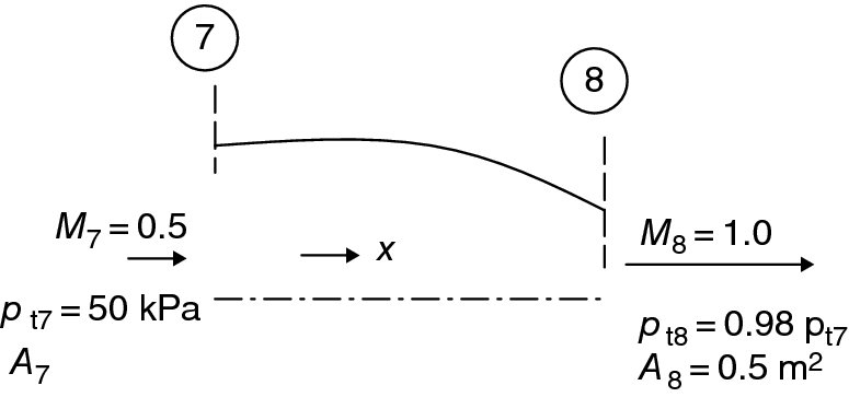
3.17 A convergent nozzle is perfectly expanded with exit Mach number M8 = 1 0. The exit total pressure is 98% of the inlet total pressure. The nozzle inlet Mach number is M7 = 0.5 and the nozzle area at the exit is A8 = 0.5 m2.
Assuming the gas ratio of specific heats is γ = 1.33, and the flow is adiabatic, calculate
nozzle inlet area A7 in m2
nozzle inlet impulse I7 in kN
nozzle exit impulse I8 in kN
the axial force (i.e., in the x-direction) exerted by the fluid on the nozzle
3.18 A turboprop engine flies at V0 = 200 m/s and produces a propeller thrust of Fprop = 40 kN and a core thrust of Fcore = 10 kN. Engine propulsive efficiency ηp is 85%. Calculate
total thrust produced by the turboprop in kN
thrust power in MW
shaft power produced by the engine ℘s in MW
3.19 A turbojet engine produces a net thrust of 40, 000 N at the flight speed of V0 of 300 m/s. For a propulsive efficiency of ηp = 0.40, estimate the turbojet exhaust speed V9 in m/s.
3.20 Calculate the engine specific impulse in seconds for Problem 3.19. Also, assuming the fuel heating value is 42, 000 kJ/kg and the thermal efficiency is 45%, estimate the fuel-to-air ratio consumed in the burner.
3.21 A turbojet engine is shown in cruise condition. The flight condition is known to be: M0 = 2.0, p0 = 20 kPa, T0 = −35°C with γ = 1.4 and R = 287 J/kg.K. The air mass flow rate into the engine is known to be . The fuel flow rate to the combustor is with heating value QR = 42, 800 kJ/kg. If the nozzle is perfectly expanded and the exhaust velocity is V9 = 1, 200 m/s, calculate:
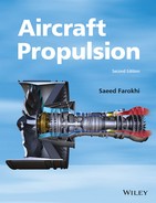

 FIGURE 3.1 Station numbers for an afterburning turbojet engine


 , first show that the contribution of the net kinetic power produced by the engine
  is small compared to the shaft power ℘s in denominator of Equation 3.56. Second, estimate the propulsive efficiency ηp for the turboprop engine from this equation.


 . The fuel flow rate to the combustor is
  with heating value QR = 42, 800 kJ/kg. If the nozzle is perfectly expanded and the exhaust velocity is V9 = 1, 200 m/s, calculate:

