7.5 Chemical Kinetics
So far our study of the chemical reactions involved an equilibrium state where the forward and reverse reaction rates were equal. However, the time it takes to reach the equilibrium state was not explicitly studied. To study the (time) rate of formation of product species in a chemical reaction, or equivalently the rate of disappearance of reactants in a reaction, is the subject of chemical kinetics. As a propulsion engineer, why should you be interested in chemical kinetics? The short answer is that it gives you an important characteristic timescale of the problem, which may affect the size and efficiency of your combustion chamber. For example, you will need to design the combustion chamber (as in a supersonic combustion ramjet) such that the residence time of species in the chamber is longer than the characteristic chemical reaction timescale for the heat of reaction to be fully realized. Also, we learn that the reaction rate depends on the pressure of the mixture, which at high altitudes (low pressures) may become too slow to effect a combustor relight. Finally, the study of chemical kinetics helps combustion engineers meet the low-pollution design objectives of low NOx, low CO, soot, and (visible) smoke dictated by the regulatory organizations (e.g., EPA and ICAO).
The cornerstone of chemical kinetics is the law of mass action, which for the following generic reaction
may be written as
that depicts the forward reaction rate. The reaction rate coefficient kf is independent of reactant’s concentration (note that the concentrations are already accounted for in the law of mass action itself) and in general is a function of pressure and temperature. The temperature dependency of the rate coefficient is in the form proposed by Arrhenius to be the Boltzmann factor (from the kinetic theory of gases), which is equal to the fraction of all collisions (i.e., the number of collisions per unit time and volume) with an energy greater than, say Ea, namely,
where Ea is the activation energy (for the reaction, which is the minimum energy to cause a chemical reaction to occur), ![]() is the universal gas constant, and T is the reactant’s absolute temperature. The activation energy for the combustion of hydrocarbon fuel in air is in the range of 40–60 kcal/mol. The frequency of the collisions, per unit volume, contributes to the reaction rate most directly and hence the pressure dependence of the reaction rate coefficient is revealed. In general,
is the universal gas constant, and T is the reactant’s absolute temperature. The activation energy for the combustion of hydrocarbon fuel in air is in the range of 40–60 kcal/mol. The frequency of the collisions, per unit volume, contributes to the reaction rate most directly and hence the pressure dependence of the reaction rate coefficient is revealed. In general,
which is called the Arrhenius rule, in honor of the man who first proposed the exponential dependence, the Boltzmann factor, for the chemical reaction rate. The exponent n on the pressure term depends on the number of molecules involved in a collision to produce the chemical reaction. For example, the combustion of hydrocarbon fuels in air involves the collision of two molecules, namely, oxygen and the fuel, hence n ≈ 2. More complex reactions involving collisions of more than two molecules in a chemical reaction lead to a higher pressure exponent n such as 3 or 4.
Now, let us examine the impact of a chemical kinetic study on a practical problem in aircraft propulsion.
7.5.1 Ignition and Relight Envelope
As noted earlier, the pressure dependence of the reaction rate coefficient may cause a relight problem at high altitude. A relight zone is plotted in Figure 7.8 in an altitude–Mach number plot (i.e., flight envelope) for the combustion of a typical hydrocarbon fuel in air (Henderson and Blazowski, 1989). We note that below 0.2 atm pressure, combustor relight is not possible at standard temperature, due to low reaction rate.

 FIGURE 7.8 The typical ignition/relight envelope shows relight capability in the shaded zone. Source: Henderson and Blazowski 1989. Reproduced with permission from AIAA
7.5.2 Reaction Timescale
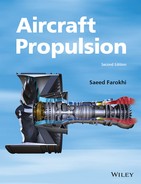
The reaction timescale and its relation to the residence timescale of the air–fuel vapor mixture control the combustion efficiency. We require that the two timescales to be equal, to establish a minimum length requirement of the combustor. A typical variation of reaction timescale with equivalence ratio for gasoline–air combustion is shown in Figure 7.9 (from Kerrebrock, 1992). This shows that near stoichiometric combustion, ![]() ∼ 1, the reaction time reaches a minimum of ∼0.3 ms. The minimum reaction timescale is one of the indicators of the desirability of stoichiometric combustion. We shall see in the next section that the flammability limit of most fuels is a narrow band centered on the stoichiometric mixture ratio of
∼ 1, the reaction time reaches a minimum of ∼0.3 ms. The minimum reaction timescale is one of the indicators of the desirability of stoichiometric combustion. We shall see in the next section that the flammability limit of most fuels is a narrow band centered on the stoichiometric mixture ratio of ![]() = 1.
= 1.
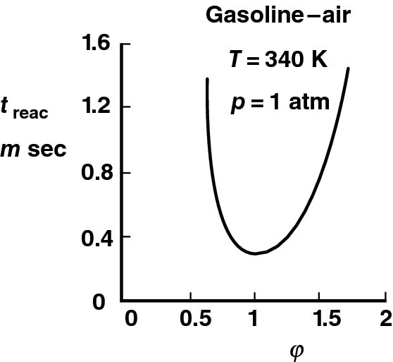
FIGURE 7.9 Reaction timescale for gasoline–air combustion as a function of equivalence ratio (Mixture at 1 atm pressure and 340 K temperature). Source: Kerrebrock 1992. Fig. 4.41. Reproduced with permission from MIT Press
The reaction timescale is inversely proportional to reaction rate (Equation 7.67), which may be written as
There are no universal rules for the pressure and temperature exponents, n and m, in a gas turbine combustor, but typical value of n is ∼1–2 and m is ∼1.5–2.5 (Zukoski, 1985). The aircraft gas turbine combustor or afterburner is designed for a residence timescale in the primary zone or the flameholder recirculation zone-mixing layer to be long compared with the reaction timescale. Hence, we are not reaction-time-limited in a conventional combustor or afterburner. However, in a scramjet combustor with a Mach 3 combustor inlet flow, we are residence-time-limited, hence reaction timescale becomes especially critical. Fortunately, the fuel of choice, hydrogen, offers not only a regenerative cooling option for the engine inlet, combustor, and nozzle but also ∼1/10 of the chemical reaction timescale of hydrocarbon fuels. The pollutant formations and their dependence on the combustor characteristic timescales will be discussed in section 7.7 in this chapter.
7.5.3 Flammability Limits
A practical aspect of combustor design examines the issues of flammability limits of various fuel–air mixture ratios as a function of temperature and pressure in a quiescent environment. It is learned that a fuel–air mixture of equivalence ratio leaner than 0.6 and richer than 3.0 will not react (i.e., sustain combustion) in room temperature and pressure, as shown in Figure 7.10 (Blazowski, 1985). In reality, a narrow band around a stoichiometric fuel–air mixture ratio is our open window for a sustained combustion. With the increase in temperature, the flammability limit boundary widens to 0.3 < ![]() < 4.0 in the spontaneous ignition temperature range (T 225°C) for a kerosene-air mixture. The flammability limits of different fuel–air mixtures, in percentage stoichiometric, are shown in Table 7.5 at the temperature of 25 °C and 1 atm pressure. The most remarkable is the wide flammability limits of hydrogen. Also hydrogen, methane, and propane enjoy very large heating capacity making them suitable coolants for active cooling of the engine and airframe structure of a hypersonic aircraft.
< 4.0 in the spontaneous ignition temperature range (T 225°C) for a kerosene-air mixture. The flammability limits of different fuel–air mixtures, in percentage stoichiometric, are shown in Table 7.5 at the temperature of 25 °C and 1 atm pressure. The most remarkable is the wide flammability limits of hydrogen. Also hydrogen, methane, and propane enjoy very large heating capacity making them suitable coolants for active cooling of the engine and airframe structure of a hypersonic aircraft.
![]() TABLE 7.5 Flammability Limits of Some Fuels(25°C and 1 atm pressure)
TABLE 7.5 Flammability Limits of Some Fuels(25°C and 1 atm pressure)
| Fuels | Jet A kerosene | Propane C3H8 | Methane CH4 | Hydrogen H2 |
| Flammability limits (percent stoichiometric) | 52–400 | 51–280 | 46–164 | 14–250 |
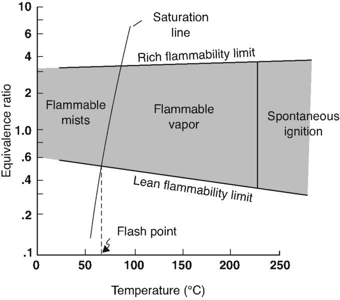
FIGURE 7.10 Flammability limits of a kerosene-type fuel in air at atmospheric pressure. Source: Blazowski 1985. Reproduced with permission from AIAA
The effect of low ambient pressure (corresponding to high altitude) on flammability limit of gasoline–air mixtures is shown in Figure 7.11 (from Olson, Childs, and Jonash, 1955). We note that the lean flammability limit at altitude approaches the stoichiometric ratio, that is, ![]() ≈ 1. We also observe that the rich flammability limit becomes much wider with the increase in pressure.
≈ 1. We also observe that the rich flammability limit becomes much wider with the increase in pressure.
FIGURE 7.11 Flammability limits of gasoline-air mixtures as a function of combustion pressure. Source: Olson et al. 1955. Fig. 1, p. 606. Reproduced with permission from ASME
As noted earlier, the flammability limits are defined for a fuel–air (gas phase) mixture as a function of temperature and pressure in a quiescent environment. In the presence of flow, combustion instabilities may set in to cause a flame blowout. Hence, the presence of a flow may drive an otherwise stable combustion (in the flammable zone) into an unstable reaction where the combustion efficiency goes to zero at the point of flame blowout. In order to sustain combustion in the presence of flow, that is, to avoid blowout, we need to employ flame stabilization schemes, which are suitable for the primary combustors and the afterburners. We will address several stabilization schemes in this chapter.
A need for an external source of energy release, as provided by an electric spark discharge, is (implicitly) demonstrated in the flammability limit diagram of kerosene–air mixture in Figure 7.10. Note that below the spontaneous ignition temperature (SIT) of the fuel–air mixture (of ∼225°C), the mixture that is defined as flammable will not self-ignite. Hence, an ignition source that is an intense localized heat source is needed to initiate the reaction. The intense localized energy release will raise the temperature of a pocket of the vaporized fuel–air mixture to a temperature above the SIT. A flame front signifying the chemical reaction zone is then formed, which propagates in the flammable mixture at a finite speed ST. Table 7.6 contains the spontaneous ignition temperature of some common fuels for reference (from Gouldin, 1973). A high spontaneous ignition temperature is desirable for a fuel that is to be used for its cooling capacity. For example, propane in Table 7.6 has the highest SIT at 767 K, which makes it a good candidate for cooling purposes. Since the spontaneous ignition temperature of fuel–air mixtures is a strong function of mixture pressure, the SIT information contained in Table 7.6 needs to be viewed with caution and not to be used for the “general purpose” fuel system safety calculation. The minimum external energy (stimulus) needed to initiate a reaction is a function of the equivalence ratio as well as the type of fuel for vaporized fuel–air mixtures. Figure 7.12 (from Lewis and von Elbe, 1961) shows the level of ignition energy of various vaporized fuel–air mixtures as a function of equivalence ratio. The ignition energies are in the form of ”bucket” shapes with the minimum ignition energy corresponding to a particular equivalence ratio.
![]() TABLE 7.6Spontaneous Ignition Temperatures of Common Fuels
TABLE 7.6Spontaneous Ignition Temperatures of Common Fuels
| Fuel | SIT (K) | Fuel | SIT (K) |
| Propane | 767 | Decane | 481 |
| Butane | 678 | Hexadecane | 478 |
| Pentane | 558 | Isooctane | 691 |
| Hexane | 534 | Kerosene (JP-8 or Jet A) | 501 |
| Heptane | 496 | JP-3 | 511 |
| Octane | 491 | JP-4 | 515 |
| Nonane | 479 | JP-5 | 506 |
Source: Adapted from Gouldin 1973.

FIGURE 7.12 Minimum ignition energy of various vaporized fuel–air mixtures. Source: Lewis and von Elbe 1961. Reproduced with permission from Elsevier
Note that in Figure 7.11, the minimum ignition energy points on the ”buckets” shifts to the right, that is, toward higher equivalence ratios, with higher molecular weight fuels. Methane, CH4, has a molecular weight of 16 and the minimum ignition energy around the stoichiometric ratio, whereas n-heptane, C7H16, has a molecular weight of 100 and the minimum ignition energy occurring around an equivalence ratio of ∼2. We may express this observation in terms of the specific gravity of these fuels as well where methane’s specific gravity is 0.466 (a light fuel) and n-heptane’s specific gravity is 0.684 (a relatively heavier fuel).
7.5.4 Flame Speed
There are two types of flames, premixed flames and diffusion flames. When the fuel and oxidizer are in gaseous form and premixed into a (stoichiometric) flammable mixture prior to combustion initiation, the resulting flame is called a premixed flame (e.g., Bunsen burner). When the fuel and oxidizer are initially separated, as in a candle burning in air, the combustion takes place within a diffusion flame zone where the vaporized fuel diffuses outward and meets an inwardly diffusing oxidizer. For an aircraft application where space is at a premium, a premixed flame combustor with a high level of turbulence intensity is the desirable choice. The effect of turbulence intensity is to promote mixing enhancement. It is the rapid and efficient mixing of the vaporized fuel–air mixture in a combustion chamber that is a performance limiting parameter, that is, limiting the energy release rate, rather than the chemical reaction timescale or flame propagation speed in conventional burners. The flame zone in a premixed combustor starts propagating initially as a laminar flame and later develops into a turbulent flame. A schematic drawing of a laminar premixed flame and its typical characteristic parameters (thickness, propagation speed, temperature range, pressure drop, and wave angle, α) are shown in Figure 7.13. The laminar flame parameters in Figure 7.13 are extracted from Borman and Ragland (1998). SL is the laminar flame speed, δL is the flame thickness, and α is the relative flow angle.

FIGURE 7.13 A schematic drawing of a thin premixed laminar flame propagating in a stoichiometric mixture of a hydrocarbon fuel and air at 1 atm pressure and T = 25° C
The initial mixture temperature has the most pronounced effect on laminar flame speed. The burning velocity of the laminar flame zone increases nearly fourfold when the initial mixture temperature is raised from 200 to 600 K, as reported by Dugger and Heimel (1952) for methane (CH4), propane (C3H8), and ethylene (C2H4) combustion in air. The mixture pressure has a minor effect on the laminar flame speed as discussed by Lefebvre (1983). The experimental results of Jost (1946), shown in Figure 7.14, demonstrate the equivalence ratio of the laminar flame speed. Moreover, they confirm the typical speed of ∼0.5 m/s for a hydrocarbon fuel, as in propane. They also show nearly an order of magnitude increase in laminar flame speed for hydrogen, which reconfirms the status of hydrogen as an ideal fuel.

FIGURE 7.14 Laminar flame speed for propane and hydrogen as a function of equivalence ratio. Source: Jost 1946
The effect of turbulence on premixed flame speed is to enhance momentum transfer between the burning front and the unburned reactants. In addition, turbulence increases the total surface area of the flame and hence increases the heat transfer between the reaction zone and the unburned gas. To visualize the surface area of a flame front under the influence of turbulence, a wrinkled flame front is proposed. Under this scenario, large (energetic) turbulent eddies strike the flame front and wrinkle the surface, while small-scale turbulence changes the transport properties within the flame zone. Figure 7.15 shows a representative drawing of a wrinkled flame front with a range of turbulent eddy sizes within the flame (adapted from Ballal and Lefebvre, 1975). Consequently, the flame propagation speed is increased from the laminar flame speed SL to the turbulent flame speed ST. The first model, due to Damkohler (1947), proposes enhancing the laminar flame speed by adding the root mean square of the turbulent fluctuation speed. The increase in flame surface area due to turbulence is proportional to

FIGURE 7.15 Graphical depiction of a wrinkled turbulent flame with a distribution of eddies within the flame. Source: Adapted from Ballal and Lefebvre 1975. Reproduced with permission from the Royal Society
The laminar flame speed is SL ∼ 0.5–2 m/s (depending on the initial mixture temperature), which is now enhanced by turbulent fluctuations. A low turbulence intensity environment, of say 5%, in a (fuel–air mixture) flow of ∼50–100 m/s results in a root mean square of the turbulent fluctuation speed of 2.5–5 m/s. Now, in a high turbulence intensity environment, of say 15–30%, in a flow with a mean speed of ∼100 m/s, the turbulence contribution to flame propagation speed may be as high as 30 m/s. Although the simple model of Damkohler in Equation 7.69 does not account for turbulence scale, the thickness of the reaction zone and other effects such as flame stretching, it serves the purpose of demonstrating the attractiveness of turbulence-enhanced mixing and its impact on the reaction timescale. A review of more elaborate models is beyond the scope and intention of the present treatment. Excellent books on combustion, such as those authored by Lefebvre (1983), Kuo (1986), Glassman (1987), Borman and Ragland (1998), among others, are recommended for further reading in this fascinating field.
7.5.5 Flame Stability
Does a Bunsen burner or a candle in a laboratory produce a stable flame? The obvious answer is yes, but the correct answer should be a conditional yes or a maybe. Since we did not specify any source or intensity of airflow in the room, we could not rule out the possibility of flame extinction caused by the airflow. If we place a Bunsen burner or a candle in a duct (for measurement purposes) connected to a fan on one side, we may experimentally establish the wind speed in the duct that causes the candle flame to blowout. Similar experiments may be conducted in a premixed combustible mixture where a flame front is established and propagates in the mixture at the flame speed S. Now, if we set the premixed gas into motion at speed U in the opposite direction to S and equal to it in magnitude, we shall achieve a stationary flame front. Simply adding the velocity vectors demonstrates the principle. For a given mixture fuel–air ratio, we may repeat the experiment for different flow speeds until we achieve an extinction of the flame (i.e., at the blowout speed). We may subsequently vary the fuel–air mixture ratio from a lean limit where extinction occurs to a rich limit at a given flow speed. The result of this experiment may be plotted in terms of the fuel–air mixture (or equivalence ratio) and the flow speed (or air mass flow rate, which is proportional to flow speed) in what is known as a stability plot or the stability loop, due to its shape. Figure 7.16 shows the combustion system stability loop for a constant pressure (from Lefebvre, 1983).

FIGURE 7.16 A typical stability loop for a combustor at p3 = constant. Source: Lefebvre 1983. Reproduced with permission from Taylor and Francis Group LLC, a division of Informa plc
The lower branch of the stability loop is the lean extinction limit and the upper branch is the rich extinction limit of combustion chamber. The maximum blowout speed occurs at the maximum flame speed, which is usually near the stoichiometric mixture ratio. The effect of pressure on the lean stability limit is negligible and widens the rich stability limit with the increase in pressure.
A recirculation zone in the burner (with a backward flow) is needed to stabilize a premixed flame. In studying swirling jets, we learn that when the ratio of jet angular momentum to jet axial thrust times jet diameter exceeds ∼0.5, a recirculatory flow in the core of the swirling jet is established. This is known as a vortex breakdown. A schematic drawing of a swirling jet with vortex breakdown is shown in Figure 7.17.
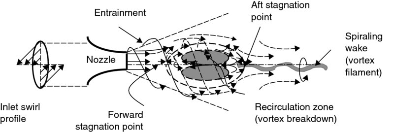
FIGURE 7.17 The flow pattern of a (bubble-type) vortex breakdown in a swirling jet
Flow visualization (via dye injection in water) of a bubble-type vortex breakdown is shown in Figure 7.18 (from Sarpkaya, 1971). The complex network of vortex filaments winding in and out of the bubble and a spiraling wake formation indicates filling and emptying of the bubble. This environment, that is, the recirculation and intense mixing of a vortex breakdown, comes close to a model of a perfectly stirred reactor that is often used in combustion studies.

FIGURE 7.18 Flow visualization of a bubble-type vortex breakdown. Source: Sarpkaya 1971. Reproduced with permission from Cambridge University Press
To help stabilize the flame in the primary zone of a main burner, air is introduced through single or double rows of swirl vanes. Also, to create a perfectly stirred reaction zone in the main burner, part of the excess air is injected into the burner through the primary air holes as radial jets. When opposing radial jets collide, a stagnation point is created with the resultant streams directed along the axis in the upstream and downstream directions. The opposing flows of the axial jet moving upstream and the spiraling air–fuel mixture create a recirculation zone with intense mixing. The combustor primary zone may also be modeled as a perfectly stirred reactor. A schematic drawing of radial jets and subsequent axial jet formations are shown in Figure 7.19.
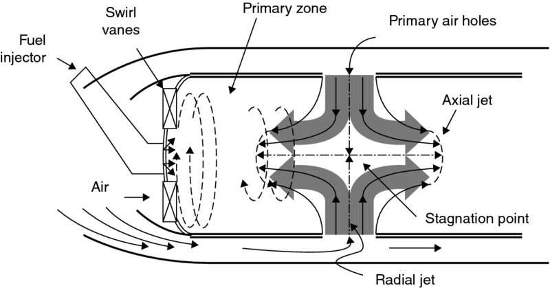
FIGURE 7.19 Collision of radial jets, stagnation point, and axial jet formation with a reverse flow in the primary zone of the combustion chamber
In an afterburner, the necessary recirculation zone to stabilize the premixed flame is created by the massively separated wakes of bluff bodies. Some geometric examples of bluff bodies that create massively separated wakes are produced in Figure 7.20.
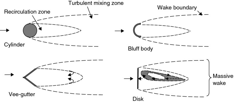
FIGURE 7.20 Bodies that create recirculation and massive wakes (suitable for subsonic flameholding)
The flameholding, that is, creating a reversed flow environment, in a high-speed scramjet combustor may be achieved by a direct fuel injection in the supersonic air stream, or via a backward-facing step. The former involves a bow shock, and the latter involves the corner flow separation. These flowfields are of interest in high-speed propulsion and are shown in Figure 7.21.
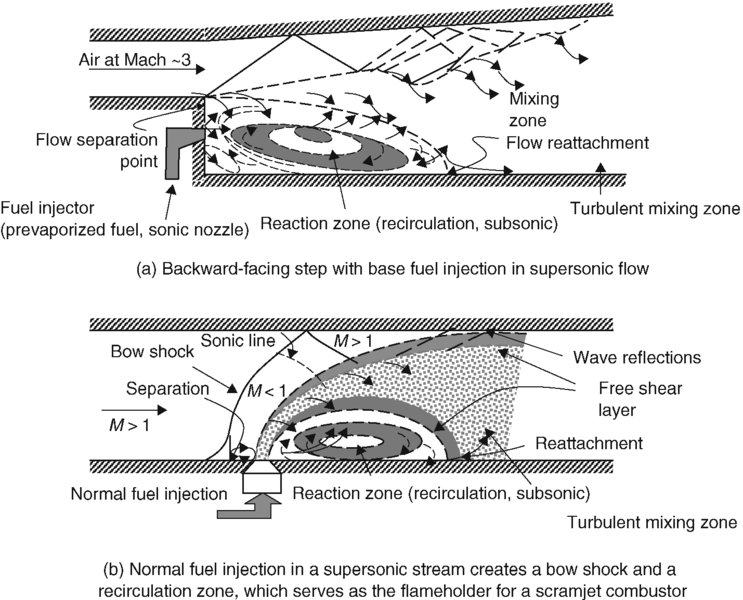
FIGURE 7.21 Fuel injection schemes in high-speed flow
The primary zone of a burner and the wake of a bluff body in the afterburner are modeled as a perfectly stirred reactor where the reactants and products are mixed infinitely fast. Such an environment produces the maximum energy release (due to infinitely fast chemical reaction rates) for the given volume of the reactor and at a fixed reactor pressure. The theory of perfectly stirred reactor has many applications, among which the stability of premixed turbulent flames in a flow environment. The perfectly stirred reactor theory predicts
where the mass flow rate in the reactor is ![]() , volume of the reactor is V, pressure of the reactor is p, the exponent of pressure represents the order of reaction, which is close to 2, and
, volume of the reactor is V, pressure of the reactor is p, the exponent of pressure represents the order of reaction, which is close to 2, and ![]() is the equivalence ratio of the fuel–air mixture. The parameter on the right-hand side of Equation 7.70 is called the combustor loading parameter (CLP). A graph of Equation 7.70 is shown in Figure 7.22 (from Spalding, 1979). A lean and a rich extinction limit (i.e., when flame instability causes extinction) are observed in Figure 7.22, similar to the stability loop of Figure 7.16. The pressure exponent “n” is taken as 1.8 in Figure 7.22, and the dimensions of the combustor loading parameter are lbm/(s · atm1.8 · ft3) in English units.
is the equivalence ratio of the fuel–air mixture. The parameter on the right-hand side of Equation 7.70 is called the combustor loading parameter (CLP). A graph of Equation 7.70 is shown in Figure 7.22 (from Spalding, 1979). A lean and a rich extinction limit (i.e., when flame instability causes extinction) are observed in Figure 7.22, similar to the stability loop of Figure 7.16. The pressure exponent “n” is taken as 1.8 in Figure 7.22, and the dimensions of the combustor loading parameter are lbm/(s · atm1.8 · ft3) in English units.
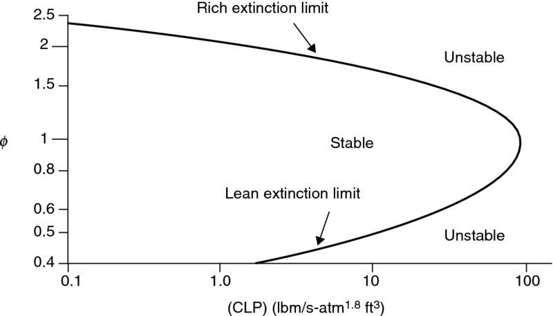
FIGURE 7.22 Combustor stability loop in terms of the loading parameter and the equivalence ratio  . Source: Spalding 1979. Reproduced with permission from Elsevier
Fundamental contributions to understanding flame stability are due to the works of Longwell, Chenevey, and Frost (1949), Haddock (1951), and Zukoski–Marble (1955). Although, we will briefly address the afterburner stability in this chapter, these references are recommended for further reading.
7.5.6 Spontaneous Ignition Delay Time
In continuing with our studies of combustion timescales and the role of chemical kinetics, we enter a new characteristic timescale, namely, the spontaneous ignition delay time. Spontaneous ignition delay time is defined as the time elapsed between the injection of a high-temperature fuel–air mixture and the appearance of a flame in the absence of an ignition source. There are two factors that contribute to an autoignition delay time. First is the rate of evaporation of fuel droplets, and the second is the chemical reaction time of the vaporized fuel and air. To promote the rate of evaporation, a liquid fuel has to be efficiently atomized to a fine spray mist. Modern aircraft engine combustors utilize spray injectors that produce an atomized fuel drop size distribution in the range of 10–400 ![]() m. Rao and Lefebvre (1981) express the ignition delay time as
m. Rao and Lefebvre (1981) express the ignition delay time as
The subscript “i” stands for ignition delay, and “e” stands for evaporation timescale in Equation 7.71. Evaporation timescale in a stagnant mixture is proportional to the surface area of the liquid fuel droplet, as the heat transfer rate to the liquid is proportional to the surface area, i.e.,
where D is the liquid fuel droplet diameter, and ReD is the fuel droplet Reynolds number based on diameter of the droplet, turbulent fluctuation velocity u′ (rms), and the kinematic viscosity of the gas νg. In the presence of a highly turbulent mixture, the evaporation time is proportional to the droplet diameter to the power three halves, that is,
according to Ballal and Lefebvre (1980). The effect of turbulence is hence to increase the heat transfer and reduce the evaporation timescale. The reaction time is expressed in terms of the mixture temperature (in K), by Rao and Lefebvre (1981), as
From the chemical kinetic rate Equation 7.67, we may also deduce the reaction timescale as the inverse of the rate constant based on initial temperature T1, namely,
The ignition delay time for a range of initial temperatures between 600 and 1000 K and a range of pressures between 1 and 30 atm is shown in Figure 7.23 (adapted from Rao and Lefebvre, 1981).
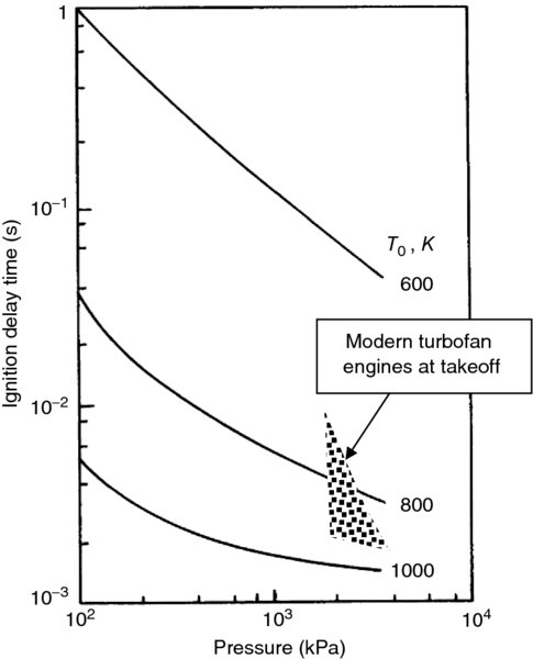
FIGURE 7.23 Effect of pressure and initial temperature on ignition delay time for a fuel–air mixture with 50  m mean diameter fuel droplet and u′ = 0.25 m/s. Source: Adapted from Rao and Lefebvre 1981
Figure 7.23 is a log–log plot. It shows an exponential drop in ignition delay time with initial temperature, as expected from Equation 7.75. The ignition delay time is also reduced with the increase in combustion pressure. This pressure dependence becomes weaker for a high inlet temperature (1000 K) and at a high pressure (30 atm). Interestingly, the conditions of 1000 K inlet temperature and 30 atm combustion pressure are representative of a typical gas turbine engine combustor inlet conditions. Based on these, the ignition delay time is ∼1–2 ms. From the reaction timescale given by Kerrebrock in Equation 7.78, we may express the pressure dependence of the ignition delay time with an inverse relation, such as
The results of autoignition delay time studies of Spadaccini (1977) for typical hydrocarbon fuels at elevated temperatures and at the pressure of 10 atm are shown in Figure 7.24 (a log–linear plot). We again observe an exponential drop in ignition time delay with temperature. The pressure dependence follows Equation 7.76, or the trends shown by Rao and Lefebvre in Figure 7.23.
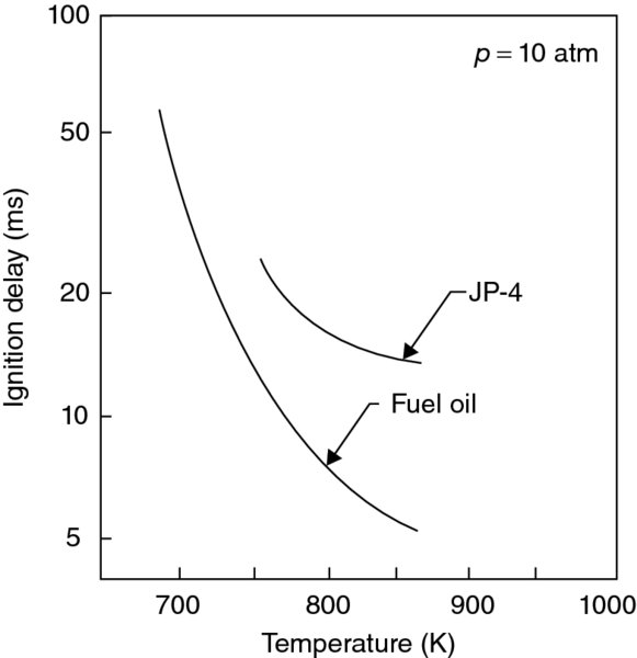
FIGURE 7.24 Spontaneous ignition delay time as a function of initial temperature at 10 atm pressure. Source: Spadaccini 1977, Fig. 9, p. 86. Reproduced with permission from ASME
7.5.7 Combustion-Generated Pollutants
The subject of pollution is an integral part of the current section, that is, chemical kinetics. However, due to its importance, this subject is presented, in more detail, after the discussion of combustion chambers and afterburners in section 7.7.
7.6 Combustion Chamber
In this section, we explore geometric configurations of combustion chambers that are found in aircraft gas turbine engines. The flammability limits of fuel–air mixtures that we studied in the last section, required a near stoichiometric mixture ratio. To prolong the turbine life, we are forced to reduce the turbine inlet temperature to levels corresponding to an equivalence ratio of ![]() ∼ 0.4–0.5. Consequently, we have to introduce the combustor inlet air in stages along the combustion chamber length. The first stage admits air in a (near) stoichiometric proportion of the injected fuel flow rate. In the first stage, air and fuel mix and chemically react in what is known as the primary zone. In the second stage, air may be used to stabilize the flame of the primary zone. The subsequent stages of air are introduced along the combustor length for dilution and cooling purposes. Proper tailoring of these stages leads to a stable combustion, reduced pollutant formation as well as a combustor exit temperature profile that is reasonably uniform and devoid of hot spots. To reduce the levels of total pressure loss in a combustor, we need to decelerate the flow at the inlet to the combustion chamber. This calls for a prediffuser.
∼ 0.4–0.5. Consequently, we have to introduce the combustor inlet air in stages along the combustion chamber length. The first stage admits air in a (near) stoichiometric proportion of the injected fuel flow rate. In the first stage, air and fuel mix and chemically react in what is known as the primary zone. In the second stage, air may be used to stabilize the flame of the primary zone. The subsequent stages of air are introduced along the combustor length for dilution and cooling purposes. Proper tailoring of these stages leads to a stable combustion, reduced pollutant formation as well as a combustor exit temperature profile that is reasonably uniform and devoid of hot spots. To reduce the levels of total pressure loss in a combustor, we need to decelerate the flow at the inlet to the combustion chamber. This calls for a prediffuser.
There are two combustor configurations that are in use in aircraft gas turbine engines, namely, the reversed-flow combustor and the straight through flow combustor. Figure 7.25 shows a schematic drawing of a reverse-flow combustor.
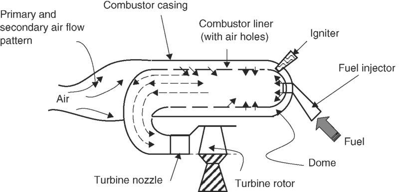
FIGURE 7.25 Reverse-flow combustor
The reverse-flow combustor is best suited for application in small gas turbine engines that utilize centrifugal compressors. The flow turns nearly 180° twice and hence it suffers an added total pressure loss due to turning over a straight through flow burner. The compact design of this burner places the turbine inlet plane near the compressor discharge plane and hence results in a shorter turbine–compressor shaft. Small airbreathing engines for drone applications as well as the early engines (e.g., Whittle engines) utilized this configuration.
A second configuration, which represents most gas turbine engines today, is the straight through flow burner. A schematic drawing of this burner is shown in Figure 7.26.
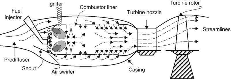
FIGURE 7.26 Schematic drawing of a straight through flow burner
The combustion chamber may be of a single-can-type tubular design, a multican design, a can-annular design, or an annular design. These configurations are shown in Figures 7.27 and 7.28.

FIGURE 7.27 Single-can, tubular, and multican combustor configurations

FIGURE 7.28 Annular combustor configurations
The single-can and the multican combustors are heavier than the latter two types of can-annular and annular combustors. The total pressure loss in these combustors is also higher than the annular types due to their larger wetted area. However, the advantages of the can type are in their mechanical robustness and their good match with the fuel injector. Coupled with a lower development cost, the single and multican systems were widely used in the early jet engines. Presently, the lowest system weight and size belong to the winner, the annular combustor, which also offers the lowest total pressure drop. The annular combustor, due to its open architecture between the fuel injectors, is more susceptible to combustion and cross-coupling-related instabilities than its counterparts with their confined configurations.
It is of critical importance to combustion system designers to understand the total pressure loss mechanisms in a combustor.
7.6.1 Combustion Chamber Total Pressure Loss
The total pressure loss in a combustor is predominantly due to two sources. The first is due to the frictional loss in the viscous layers where we can lump in the mixing loss of the fuel and air streams prior to chemical interaction. The second source is due to heat release in an exothermic chemical reaction in the burner. The first is usually modeled as the “cold” flow loss and the second is the “hot” flow loss. We recognize, however, that the subdivision of the losses into “cold” and “hot” is artificial and the two forms of total pressure loss occur simultaneously and interact in a complex way. But throughout the ages, engineering is practiced through the art of simplification, that is, engineers have broken down a complex problem into a series of elementary and solvable problems and then tried to predict the solution of the complex problem by devising a correlation between the elementary solutions and the observation or measurement. We intend to stay our engineering course on the topic of combustion chamber total pressure loss. There are several methods of quantifying the total pressure loss in a combustor, namely,
The first expression is the overall total pressure loss ratio, the second expression is a measure of the total pressure loss in terms of the inlet dynamic pressure, and the last expression uses a reference velocity for the dynamic pressure and measures the total pressure loss in terms of the reference dynamic pressure. The reference velocity is the mass averaged gas speed at the largest cross-section of the burner, based on the combustor inlet pressure and temperature. The reference Mach number is the ratio of the reference speed to the speed of sound at the prediffuser inlet a3. All the aerodynamic losses scale with reference dynamic pressure, as shown in Figure 7.29 (from Henderson and Blazowski, 1989).

FIGURE 7.29 Percentage total pressure loss in a combustor. Source: Henderson and Blazowski 1989. Reproduced with permission from AIAA
A parabolic dependence of the total pressure loss on the reference Mach number is shown in Figure 7.29. Kerrebrock suggests an empirical rule for the combustor total pressure ratio, as a fraction of reference dynamic pressure. In terms of the average Mach number of the gases in the burner, Mb, Kerrebrock’s empirical rule is stated as
where ![]() .
.
This equation states that the total pressure loss is proportional to an “average” dynamic pressure of the gases in the combustor, with the proportionality constant ![]() . We note that the total pressure loss grows as the mean flow speed increases. Now, we appreciate the role of prediffuser in a combustion chamber. The total pressure loss due to combustion that is, heat release, in the burner may be modeled by a Rayleigh flow analysis. The conservation of mass and momentum for a constant-area frictionless duct are
. We note that the total pressure loss grows as the mean flow speed increases. Now, we appreciate the role of prediffuser in a combustion chamber. The total pressure loss due to combustion that is, heat release, in the burner may be modeled by a Rayleigh flow analysis. The conservation of mass and momentum for a constant-area frictionless duct are
Now, instead of the compressible equation for the total pressure involving Mach number, we may use the low-speed version in an approximation, that is, the Bernoulli equation, namely,
Canceling the first two parentheses via momentum Equation 7.82, and using the continuity equation we may simplify Equation 7.83 as
Now, using the perfect gas law for the density ratio and neglecting static pressure changes between the inlet and exit of the burner in favor of the large temperature rise across the combustor, we may write the following simple expression for the total pressure loss due to heating in a constant-area burner as
In deriving the above expression, we made a series of approximations and simplifications. Consequently, we may use Equation 7.85 in relative terms, for example, in describing the effect of the throttle setting (T4) on the variation of (hot) total pressure loss in a burner. Lefebvre (1983) suggests a correlation based on the Equation 7.85 that involves two unknown coefficients, K1 and K2, as
The correlation coefficients K1 and K2 need to be established experimentally. This is another example of a simple model (Equation 7.85) that is the basis of an engineering correlation for a complex problem. The total pressure loss due to combustion is small compared with aerodynamic losses, namely,
The cold total pressure loss is in the range of ∼4–7%, that is,
In an afterburner, the process of flame stabilization is achieved via flameholders, as described earlier, that creates massively separated wakes and is responsible for the bulk of the total pressure loss. We model an afterburner as a constant-area duct with a series of bluff bodies in the stream with a known drag coefficient. The diagram that describes the problem is shown in Figure 7.30.
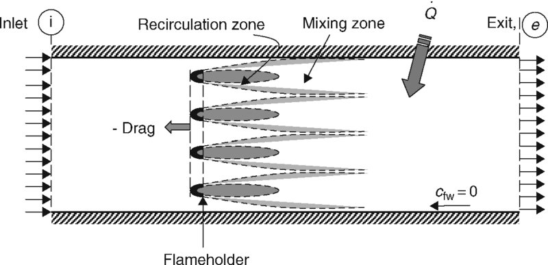
FIGURE 7.30 Control volume for the estimation of total pressure loss in an afterburner
We may account for the wall friction in the momentum balance equation either directly or we may combine its overall drag contribution with the flameholder drag. The effect of combustion on total pressure loss is important and will be investigated later in this section.
First, we model the afterburner-off condition, which is known as the “dry” analysis of the engine. The “wet” mode analysis follows the “dry” mode in this section.
From continuity equation we have
The fluid momentum equation in the streamwise direction gives
We define the flameholder drag in terms of the duct cross-sectional area A as
Rearranging the terms of the momentum equation, we get
Therefore, the static pressure ratio is expressed in terms of the inlet and exit Mach numbers and the flameholder drag coefficient CD as

From the continuity equation, we express the density ratio in terms of the velocity ratio and then we replace the gas speed by the product of Mach number and the speed of sound to get
We use the energy equation for an adiabatic process, which is a statement of the conservation of total enthalpy, to get the static temperature ratio, namely,

By invoking the perfect gas law, we link the static pressure, density, and temperature ratios of the gas at the inlet and exit of the duct as
Now, all the ratios in Equation 7.94 are expressed in terms of the inlet and exit Mach numbers and gas properties. Hence, for a known inlet condition, we may use this equation to establish the exit Mach number Me. Let us substitute expressions 7.91, 7.92, and 7.93 in Equation 7.94 to get the desired equation involving one unknown Me,

We may simplify the above equation by combining the gas properties and the last two brackets, to get
Fortunately, Equation 7.96 is aquadratic equation for Me with a closed form solution, that is, no iteration is needed. Therefore the exit Mach number is
where
With exit Mach number known, we may substitute it in Equation 7.91 to get the static pressure ratio, and the total pressure ratio is then calculated by
Now we may graph the total pressure loss, due to flameholder drag, across the afterburner, as a function of inlet Mach number and gas properties at the inlet and exit.
Figure 7.31 shows the aerodynamic impact of flameholder drag on afterburner total pressure loss. The importance of low inlet Mach number to the afterburner may also be discerned from this figure. The penalty for a high inlet Mach number (of say ∼0.5) is severe and thus the necessity of a prediffuser becomes evident. The presence of aerodynamic drag in the afterburner causes the exit Mach number to increase and approach a choked, that is, Me = 1, state. Frictional choking in the afterburner is to be avoided since combustion also tends to increase the Mach number, as in Rayleigh flow. A graph of the exit Mach number as a function of inlet Mach number and the flameholder drag coefficient is shown in Figure 7.32.
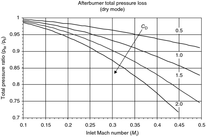
FIGURE 7.31 Afterburner total pressure loss due to flameholder drag (γi = 1.33, γe = 1.30)

FIGURE 7.32 Frictional choking of afterburner caused by flameholder drag (γi = 1.33, γe = 1.30)
The flameholder drag coefficient in our analysis was defined based on the afterburner cross-sectional area. However, the drag coefficient of bluff bodies is defined based on the maximum cross-sectional area of the bluff body. Therefore,
where the Amax is the base area of an individual bluff body and N is the number of bluff bodies used in the flameholder arrangement, typically in the form V-gutter rings and radial V-gutter connectors. We may define a flameholder blockage area ratio as
Therefore, the drag coefficient used in our afterburner total pressure loss calculation is related to the individual drag coefficients via the blockage factor, that is,
Figure 7.33 serves as a definition sketch for the afterburner duct, and the flameholder rings that contribute to the blockage parameter B. Here the radial gutters that connect the V-gutter rings to the turbine exit diffuser cone or the casing are not shown. The EJ200 of Eurojet Consortium uses radial gutters (instead of rings) for flame holding (Figure 7.47).
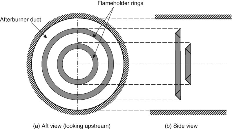
FIGURE 7.33 Schematic drawing of the afterburner duct and the flameholder rings

FIGURE 7.34 Afterburner total pressure loss variation with inlet Mach number and heat release (γi = 1.33, γe = 1.30, CD = 0.5)
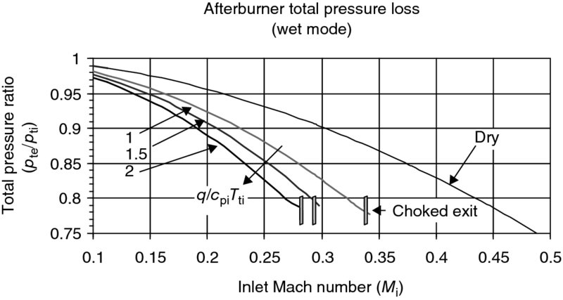
FIGURE 7.35 Afterburner total pressure loss with heat release and a higher flameholder drag (γi = 1.33, γe = 1.30, CD = 1.5)
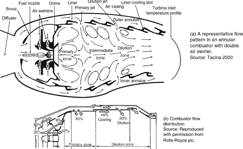
FIGURE 7.36 Flow distribution and pattern in modern combustors

FIGURE 7.37 Combustor liner cooling methods. Source: Henderson and Blazowski 1989. Reproduced with permission from AIAA

FIGURE 7.38 Combustor liner cooling techniques. Source: Henderson and Blazowski 1989. Reproduced with permission from AIAA
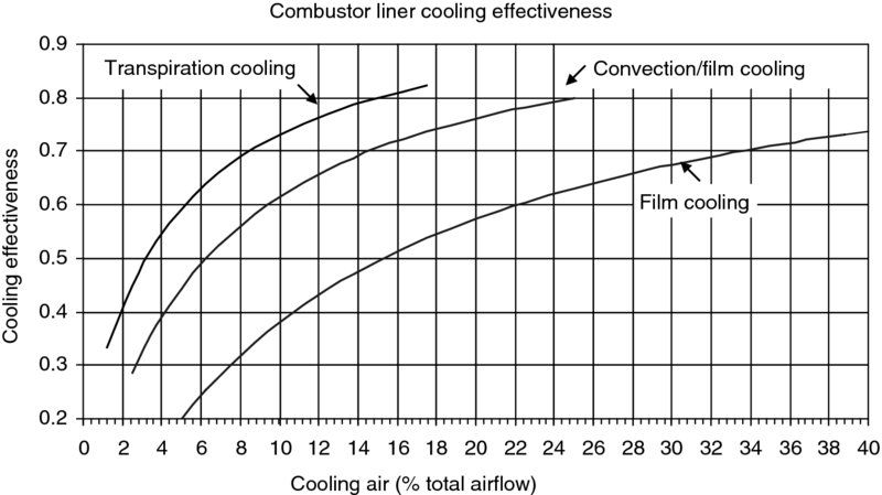
FIGURE 7.39 Combustor liner cooling effectiveness. Source: Adapted from Nealy and Reider 1980
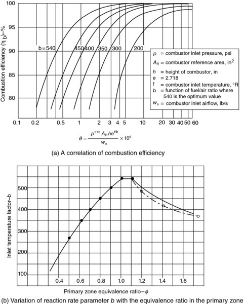
FIGURE 7.40 Combustion efficiency correlation based on Lefebvre θ parameter. Source: Henderson and Blazowski 1989. Reproduced with permission from AIAA

FIGURE 7.41 Schematic drawing of a dump diffuser

FIGURE 7.42 F101 annular combustor with a dump (pre-) diffuser design. Source: Henderson and Blazowski 1989. Reproduced with permission from AIAA

FIGURE 7.43 Total pressure ratio and exit Mach number in a dump diffuser [M1 = 0.5, γ = 1.4)
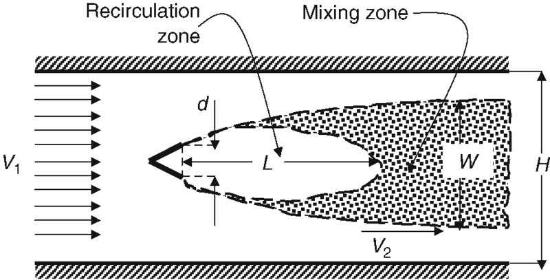
FIGURE 7.44 Length and velocity scales associated with a single flameholder in a duct

FIGURE 7.45 Comparison between theoretical stability predictions (potential flow) and the experimental data of Wright for flameholder wedge half-angles of 30° and 90° in a 2D rectangular duct. Source: Adapted from Zukoski 1985
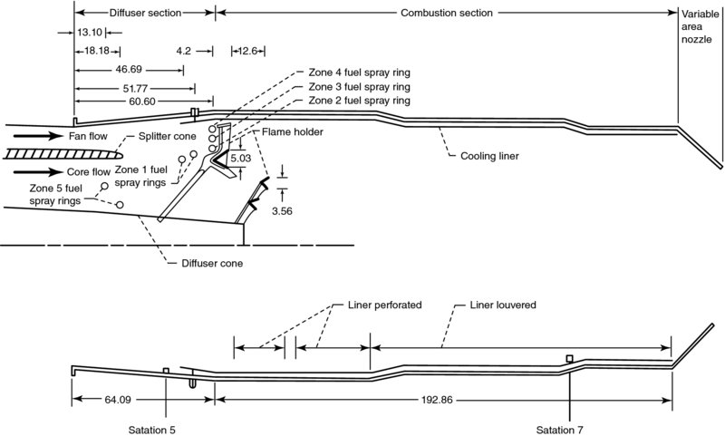
FIGURE 7.46 The TF30-P-3 turbofan engine with its afterburner showing the installation and scales of the flameholders, fuel injection rings and the diffuser cone (all dimensions in cm). Source: McAulay and Abdelwahab 1972. Courtesy of NASA
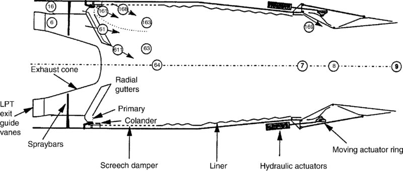
FIGURE 7.47 Longitudinal section of the EJ200 afterburner and nozzle. Source: Kurzke and Riegler 1998. Courtesy of U.S. Government
To account for higher flow velocities in the plane of the flameholder, due to flameholder blockage, the drag coefficient needs to be scaled by the dynamic pressure ratio, that is,
where subscript “fh” identifies the plane of the flameholder and the bluff body drag coefficient (e.g., a V-gutter) was assumed to be ∼1. Note that a flat plate, in broadside, creates a drag coefficient of 2 and a cylinder in cross flow ∼1.2 (both flows at a Reynolds number based on plate height or cylinder diameter of 100, 000).
The analysis of an afterburner in the “wet” mode differs from the “dry” mode only in its energy balance equation, namely,
By neglecting the fuel-to-air ratio in the afterburner in favor of 1 on the left-hand side of the energy equation and renaming the product term on the RHS as “q, ” we get
We may relate the static enthalpy ratio to the stagnation enthalpy and Mach number as

By replacing Equation 7.93 with the above equation, and proceeding with the substitution of the static pressure ratio and density ratio in the perfect gas law, we obtain
Again, the above expression involves one unknown, that is, Me, and is fortunately a quadratic equation with the following closed form solution:
where
Now, let us graph the total pressure loss in an afterburner in the wet mode (sometimes referred to as the reheat mode), using the above solution for the exit Mach number. Figure 7.34 shows the afterburner total pressure loss increases with heat release in the combustor. We also note that the choked exit condition is reached at a relatively low inlet Mach number of <0.4. Higher heating levels and flameholder drag coefficients will result in earlier choking than shown in Figure 7.34. Thus, the necessity of decelerating the flow entering an afterburner is again evident from Figure 7.34.
We produce Figure 7.35 to demonstrate the effect of higher flameholder drag coefficient on the afterburner wet mode total pressure loss, and the inlet Mach number range that leads to exit choking. Based on these results, an inlet’s Mach number range of ∼0.2–0.25 is desirable for an afterburner.
7.6.2 Combustor Flow Pattern and Temperature Profile
A typical flow pattern in a primary burner is demonstrated in Figure 7.36a (from Tacina, 2000), which shows the burner primary zone, intermediate zone, and the dilution zone in an annular combustor. We have already discussed the primary zone in the context of flammability, flame stability, and stoichiometry. The primary air jets in opposing radial directions are also introduced to stabilize the flame and increase combustor efficiency/heat release rate. The role of intermediate zone is seen as an extension of the primary zone in achieving a complete combustion/controlling pollutant formations, and the dilution zone is seen as producing a desired turbine inlet temperature profile, as shown in Figure 7.36a. Airflow distribution in a modern combustor is shown in Figure 7.36b.
The temperature profile at the turbine inlet exhibits nonuniformity due to the number of fuel injectors used in the circumferential direction, the nonuniformity in dilution air cooling and mixing characteristics as well as other secondary flow patterns and instabilities that are set up in the burner. These spatial nonuniformities at combustor exit are described by two nondimensional parameters, the pattern factor and the profile factor.
Pattern factor
where Tt-max is the absolute maximum exit temperature in the circumferential and radial directions, Tt-avg is the average of the exit temperature, and Tt-in is the average inlet total temperature. Since the nonuniformity parameter in the numerator of Equation 7.110 is the absolute maximum of the exit temperature (i.e., the absolute peak), this parameter is also known as the peak temperature factor. Turbine nozzle is exposed to this nonuniformity. The desired range of this parameter is between 0.15 and 0.25 in modern high-temperature rise combustors.
Profile factor
where Tt-max-avg is the circumferential average of the maximum temperature, that is, the average of all the local peaks in the circumferential direction. Since the flow acceleration in the turbine nozzle reduces the temperature distortion levels, the turbine rotor that follows the nozzle is exposed to this nonuniformity. The range of this parameter is between 1.04 and 1.08.
REMARKS Flow acceleration dampens nonuniformity in the flow, whereas flow deceleration amplifies distortion. Therefore, the temperature distortion at the turbine inlet is reduced after the nozzle. By the same token, the flow distortion in the inlet diffuser or in the compressor blades is amplified. All engineers dealing with fluid flow problems should know this principle. The proof of this principle is very simple using a parallel flow model (see Problem 7.22).
7.6.3 Combustor Liner and Its Cooling Methods
Combustion takes place inside a combustor liner. It consists of a dome in the primary zone, primary air holes for the primary (radial) jets, air holes for the intermediate zone (radial jets), and the cooling holes/slots in the dilution zone. The combustion temperature may exceed 2500 K (in the primary zone), whereas the liner temperature needs to be kept at ∼1200 K. The heat transfer to the liner from the combustion side is in the form of radiation and convective heating by the hot combustion gases. The conventional cooling techniques used in gas turbine engines are
- Convective cooling
- Impingement cooling
- Film cooling
- Transpiration cooling
- Radiation cooling
- Some combination of the above.
The convective cooling method is primarily used in cooled turbine blades with the philosophy of maximizing the heat transfer rate from a hot wall (gas side) to the coolant inside the blade. The coolant may also impinge on a hot surface to create a stagnation point and hence enhance the heat transfer to the coolant through the wall. The impingement cooling method is often used in the leading-edge cooling of turbine blades. The film cooling method operates on the principle of minimizing heat transfer to the wall from the hot gases by providing a protective cool layer on the hot surface. The cool layer acts like a “blanket” that protects the surface from the hot gases. In film cooling, the coolant is injected through a series of discrete fine film holes, at a slanted angle to the flow direction, and emerges on the hot side to provide the protective cooling layer. Note that the philosophy of film cooling to minimize heat transfer to a wall is different from that of convective cooling, which maximizes the heat transfer through a wall. The transpiration cooling calls for a porous surface where the coolant emerges on the hot gas side through the pores. The cooling protection that it provides is similar to the film cooling technique, that is, by blanketing the surface with a coolant layer. Transpiration cooling may be viewed as the ultimate film cooling in the limit of infinitely many and continuously distributed film holes on a surface. Finally, the radiation cooling accompanies all surfaces above the absolute zero temperature. The radiation cooling of the liner to the outer casing, however, represents only a small fraction of the overall heat transfer of the liner. We shall discuss these in the context of cooled turbine blades and shrouds in more detail in Chapter 10.
The availability of excess air at the burner inlet dominates the application of these heat transfer techniques to a combustor liner. The primary and the intermediate zone air holes are designed to provide combustion stability and maximizing the chemical reaction heat release. The remaining air, which may be about 15–30% of the combustor inlet flow, is used to provide a reliable and uniform cooling protection to the liner. A successively more sophisticated technique of liner cooling is shown in Figures 7.37 and 7.38 (from Henderson and Blazowski, 1989). Starting from the louver cooling with the problems of uniform coolant distribution and control that marked the early combustor development to the most sophisticated transpiration cooling are schematically shown in Figure 7.37.
The coolant mass flow requirement is diminished with cooling effectiveness. Simple film cooling, convection/film, impingement/film, and the transpiration cooling are ranked from the highest to the lowest coolant requirement, respectively. The film cooling method eliminates the problem of coolant injection uniformity and control that was shown by louver technique. The combination convection/film and impingement/film cooling techniques offer a further enhancement of cooling effectiveness of the combustor liner. The transpiration cooling through a porous liner minimizes the coolant flow requirement and offers the most uniform wall temperature distribution (Figure 7.38). The problem of pore clogging, however, poses a challenge in transpiration cooling.
To quantify the coolant mass flow requirement, we define a cooling effectiveness parameter Φ according to
The cooling effectiveness is the ratio of two temperature differentials. The numerator is the difference between the hot gas Tg and the desired (average) wall temperature Tw. The denominator represents the absolute maximum potential for wall cooling. Therefore, the cooling effectiveness Φ is the fraction of the absolute maximum cooling potential that is realized in the wall cooling process. The hot gas in this application is the combustion temperature (Tg) or sometimes referred to as the flame temperature, and the coolant is the compressor discharge temperature (Tc). The desired wall temperature Tw is dictated by the wall material properties and durability requirements (e.g., 18, 000 or 20, 000-hr life). The variation of cooling effectiveness with coolant flow is shown in Figure 7.39 (data from Nealy and Reider, 1980).
In future advanced gas turbine engines, the combustor temperature may reach ∼2500 K (near the maximum adiabatic flame temperature of hydrocarbon fuels), with a desired liner temperature of ∼1200 K and a compressor discharge temperature of 900 K, the cooling effectiveness is then 0.8125. In examining Figure 7.39, we note that a film-cooled liner may not reach this desired level of cooling effectiveness, regardless of percentage coolant available. On the contrary, this level of cooling effectiveness represents the maximum possible limit of the transpiration cooling at close to 18% coolant availability/usage. Application of a thin layer of refractory material such as a ceramic coating lowers the heat transfer to the wall and thus allows a higher operating temperature in the combustor. To tolerate a higher heat release level in an advanced combustor, the liner material needs to tolerate higher operating temperatures and require less (to no) cooling percentage. In addition to operating at high temperatures, the liner material has to be oxidation resistant. Refractory metals such as molybdenum and tungsten suffer in this regard. A promising new liner material is the ceramic matrix composite (CMC). Development of prototype CMC combustor liner has been approached in industry by using silicon carbide fiber reinforced silicon carbide (SiC/SiC). The use of advanced composite materials as combustor liners represents a challenge in manufacturing, scaling up, life prediction, damage tolerance, reparability characteristics and cost.
7.6.4 Combustion Efficiency
Combustion efficiency measures the actual rate of heat release in a burner and compares it with the theoretical heat release rate possible. The theoretical heat of reaction of the fuel assumes a complete combustion with no unburned hydrocarbon fuel and no dissociation of the products of combustion. The actual heat release is affected by the quality of fuel atomization, vaporization, mixing, ignition, chemical kinetics, flame stabilization, intermediate air flow, liner cooling, and, in general, the aerodynamics of the combustor. Here a variety of timescales as in residence time, chemical reaction/reaction rate timescales, spontaneous ignition delay time that includes vaporization timescale, among other time constants enter the real combustion problem. The unburned hydrocarbon (UHC) and carbon monoxide (CO) that contribute to combustor inefficiency are also among the combustion-generated pollutants. The allowable levels of these pollutants in aircraft gas turbine engine emissions, regulated by the U.S. Environmental Protection Agency (EPA), place a 99% combustion efficiency demand on the combustor.
For a gas turbine combustor, when chemical kinetics is the limiting factor in combustor performance, Lefebvre (1959, 1966) introduces a combustor loading parameter (CLP) θ, which correlates well with combustion efficiency. θ parameter is defined as
The combustor inlet pressure, temperature, and mass flow rate are pt3, Tt3, and ![]() 3, respectively, maximum cross-sectional area of the burner is defined as Aref, the combustor height is H and b is a reaction rate parameter. The dependence of the reaction rate parameter b on the primary zone equivalence ratio
3, respectively, maximum cross-sectional area of the burner is defined as Aref, the combustor height is H and b is a reaction rate parameter. The dependence of the reaction rate parameter b on the primary zone equivalence ratio ![]() is estimated by Herbert (1957) to be
is estimated by Herbert (1957) to be
These expressions are plotted in Figure 7.40 (from Henderson and Blazowski, 1989). Note that dimensions of the parameters used in Figure 7.40 a are in English units, as described in the definition box in the graph.
The lowest combustion efficiency is, of course, zero in the flameout limit. This could happen at a high altitude when the low combustor pressure in essence slows the reaction rate to a halt (τresidence![]() τreaction). The graphical correlations used in the combustion efficiency Figure 7.40 are then used to size the combustor in conditions corresponding to high altitude (for a relight requirement) assuming a combustor efficiency of 80%.
τreaction). The graphical correlations used in the combustion efficiency Figure 7.40 are then used to size the combustor in conditions corresponding to high altitude (for a relight requirement) assuming a combustor efficiency of 80%.
7.6.5 Some Combustor Sizing and Scaling Laws
The engine size, that is, the core (air) mass flow rate, and the compressor pressure ratio, by and large, determine the combustor inlet flow area. The flow area takes the form of an annulus, and its size is A3. We may calculate the flow area A3 by a one-dimensional continuity equation such as

At design point, the engine (core) mass flow rate, the compressor discharge parameters pt3 and Tt3 (which are a function of πc and ec), and our design choice for M3 size the flow area A3 according to Equation 7.115. A typical compressor exit Mach number is ∼0.4–0.5. However, a combustor requires a prediffuser to decelerate the air from the compressor to improve combustion total pressure (loss) and combustion efficiency. A desired combustor inlet Mach number is ∼0.2. A conventional diffuser may be designed by using the design charts that were presented in the inlet and nozzle chapter. Diffusion is a slow and patient process, which normally takes place in a long duct of shallow wall divergence angles of ∼3–5° inclination with respect to a straight centerline. To shorten the axial length of a combustor prediffuser, one may employ a
- Diffuser with splitter vanes
- Dump diffuser
- Vortex-controlled diffuser.
The subject of a wide-angle diffuser that employs splitter vanes was already presented in Chapter 6 (references 1 and 2 should be consulted on short and hybrid diffusers). In a dump diffuser, the flow area undergoes a sudden expansion with the attendant flow separation at the lip. Figure 7.41 shows a schematic drawing of a dump diffuser.
A curved turbulent shear layer emerges from the point of separation, which reattaches in approximately 5–7 inlet channel heights, for a two-dimensional expansion. A pair of stable vortex structures is formed (in 2D) at the separation corner. In the axisymmetric case, a stable vortex ring is formed at the separation junction. The expression used in Figure 7.41 for the static pressure ratio and velocity ratio is based on Bernoulli equation, and the last part that relates the flow speed to flow area is based on the incompressible continuity equation. The loss of total pressure between stations 1 and 2 is due to viscous/turbulent mixing and dissipation in the separated shear layer and the boundary layer formation downstream of the reattachment point. An example of an annular combustor using a dump prediffuser is shown in Figure 7.42 (from Henderson and Blazowski, 1989).
Total pressure recovery of a dump diffuser is a function of Reynolds number and the Mach number at its inlet. For Reynolds number based on the inlet diameter of ∼500, 000 to 106, Barclay (1972) recommends the following correlation:
The exit Mach number M2 is then established using a continuity equation, according to
The total pressure recovery of a dump diffuser and its exit Mach number are plotted in Figure 7.43 for an inlet Mach number of M1 = 0.5 and γ = 1.4.
Figure 7.43 indicates that in order to decelerate a Mach 0.5 flow to an exit Mach number of 0.2 in a dump diffuser, we need to employ an area ratio of ∼2.35, and the flow in the dump diffuser will recover ∼0.935 of its inlet total pressure (i.e., it suffers ∼6.5% loss).
To establish a length for the main combustor, we relate the residence time of the fluid in the burner to the ratio of fluid mass to the flow rate in the combustor, namely,
where Aref is the maximum cross-sectional area of the burner, L is the burner length, and the mass flow rate through the burner is estimated as the airflow rate at the combustor entrance. Now, expressing the fluid density in terms of compressor pressure ratio via an isentropic exponent, namely,
We may isolate combustor length L from Equation 7.118 and express it as
In the above expression, A2 is the engine face area and the first parenthesis is a design parameter, which is independent of the engine size. The area ratio A2![]() Aref may be related via continuity equation to the engine face axial Mach number (a design choice) and the combustor exit Mach number (i.e., taken at the exit of the turbine nozzle) M4 and the total pressure and temperature ratios according to
Aref may be related via continuity equation to the engine face axial Mach number (a design choice) and the combustor exit Mach number (i.e., taken at the exit of the turbine nozzle) M4 and the total pressure and temperature ratios according to
In Equation 7.120, the burner exit Mach number (taken at the exit of the turbine nozzle) is set equal to 1, as the turbine nozzle remains choked over a wide range of operating conditions. We may approximate the total pressure ratio term in Equation 7.120 by the compressor pressure ratio and express the combustor length L as
The fluid residence timescale and the chemical reaction timescale may be interchanged in a combustor
The reaction timescale is inversely proportional to the reaction rate and attains the following general form,
Now, substituting Equation 7.123 for the residence timescale into Equation 7.121, we get
We may combine the exponents of the compressor pressure ratio in Equation 7.124 as

This equation relates the combustor length L to cycle parameters πc and τλ, which are independent of size. Hence, a high-pressure ratio engine occupies a smaller length combustor than a comparable size engine with a lower pressure ratio. A similar argument can be made regarding the cycle thermal loading parameter τλ. Table 7.7 (from Henderson and Blazowski, 1989) shows some data on contemporary combustor size, weight, and cost.
![]() TABLE 7.7 Data on Combustor Size, Weight, and Cost
TABLE 7.7 Data on Combustor Size, Weight, and Cost
| Parameter | TF39 | TF41 | J79 | JT9D | T63 |
| Type Mass flow (design point) | Annular | Cannular | Cannular | Annular | Can |
| Airflow, lb/s | 178 | 135 | 162 | 242 | 3.3 |
| kg/s | 81 | 61 | 74 | 110 | 1.5 |
| Fuel flow, lb/h | 12, 850 | 9965 | 8350 | 16, 100 | 235 |
| kg/h | 5829 | 4520 | 3788 | 7303 | 107 |
| Size | |||||
| Length, in | 20.7 | 16.6 | 19.0 | 17.3 | 9.5 |
| cm | 52.6 | 42.2 | 48.3 | 43.9 | 24.1 |
| Diameter, in | 33.3 | 5.3/24.1a | 6.5/32.0a | 38.0 | 5.4 |
| cm | 84.6 | 13.5/61.2 | 16.5/81.3 | 96.5 | 13.7 |
| Weight, lb | 202 | 64 | 92 | 217 | 2.2 |
| kg | 92 | 29 | 42 | 98 | 1.0 |
| Cost, $ | 42, 000 | 17, 000 | 11, 300 | 80, 000 | 710 |
Source: Henderson and Blazowski 1989. Reproduced with permission from AIAA
aCan diameter/annulus diameter.
7.6.6 Afterburner
So far, we have discussed the total pressure drop in an afterburner due to flameholder drag and combustion. We also alluded to the flame stability provided by abluff-body flameholder. In this section, we quantify the parameters governed by the fluid mechanics and the chemical reaction that afford flame stability in an afterburner. We also develop a scaling parameter that connects different flameholder arrangements and duct geometries to experimental results obtained in a rectangular duct with a single flameholder. We first define a bluff body and its wake in a duct by the following length and velocity scales, as shown in Figure 7.44.
The wake of a V-gutter of height “d” is shown to have a central recirculation zone of length “L, ” a wake width “W, ” a channel height “H, ” an upstream gas velocity V1, and an accelerated gas velocity, just outside the mixing layer, V2, known as the “edge velocity.” We had defined a blockage parameter B, which for a two-dimensional duct, as shown in Figure 7.44, is the ratio B = d/H. The blockage parameter B and the wake width establish the flow acceleration V2. A continuous chemical reaction in the mixing layer will be supported only if the resident timescale of the fuel/air mixture in the mixing layer is longer than the reaction timescale. Hence, for flame stability, the following simple relationship should hold between the two characteristic timescales, namely,
This is the basis of Zukoski-Marble (1955) characteristic time model for flame stability. The resident timescale of the unburned gas is proportional to the ratio
where ![]() is an average gas speed in the mixing layer. Hence, a dimensionless parameter
is an average gas speed in the mixing layer. Hence, a dimensionless parameter ![]() emerges that could serve as a stability criterion. Experiments are conducted that establish the flame blowout condition in a rectangular duct with a single flameholder at the center of the duct with a range of chemical reaction parameters. The blowout condition parameters are labeled with a subscript “c” and by combining the proportionality constants in the unknown time constant τc, the average gas speed in the mixing layer is replaced by V2c to produce
emerges that could serve as a stability criterion. Experiments are conducted that establish the flame blowout condition in a rectangular duct with a single flameholder at the center of the duct with a range of chemical reaction parameters. The blowout condition parameters are labeled with a subscript “c” and by combining the proportionality constants in the unknown time constant τc, the average gas speed in the mixing layer is replaced by V2c to produce
as the blowout stability criterion, or the marginal stability criterion. The measurements of L and V2c then establish the critical timescale τc at the blowout condition. The ratio V2c![]() L represents the fluid dynamic parameter in Equation 7.128, whereas τc represents the effect of all chemical reaction parameters lumped into a single term. The timescale τc, which is also referred to as ignition time, is independent of the flameholder geometry and arrangement so long as the mixing layer is turbulent. It depends, however, on a number of parameters, such as the fuel-to-air ratio, fuel type, inlet temperature, and the degree of vitiation of the afterburner gas. Experimental results of Zukoski (1985) over a range of two- and three-dimensional flame-holders indicate that the τc is ∼0.3 ms at stoichiometric fuel–air ratio. This is consistent with Figure 7.9 (from Kerrebrock) that shows the reaction bucket has a minimum of ∼0.3 ms near stoichiometric ratio and up to ∼1.5 ms in fuel lean and rich limits of gasoline–air mixtures (see Figure 7.9). A more convenient stability parameter may be defined using the upstream blowout velocity V1c and the duct height H as a reference velocity and length scale,
L represents the fluid dynamic parameter in Equation 7.128, whereas τc represents the effect of all chemical reaction parameters lumped into a single term. The timescale τc, which is also referred to as ignition time, is independent of the flameholder geometry and arrangement so long as the mixing layer is turbulent. It depends, however, on a number of parameters, such as the fuel-to-air ratio, fuel type, inlet temperature, and the degree of vitiation of the afterburner gas. Experimental results of Zukoski (1985) over a range of two- and three-dimensional flame-holders indicate that the τc is ∼0.3 ms at stoichiometric fuel–air ratio. This is consistent with Figure 7.9 (from Kerrebrock) that shows the reaction bucket has a minimum of ∼0.3 ms near stoichiometric ratio and up to ∼1.5 ms in fuel lean and rich limits of gasoline–air mixtures (see Figure 7.9). A more convenient stability parameter may be defined using the upstream blowout velocity V1c and the duct height H as a reference velocity and length scale,
The length of recirculation zone to the wake width L![]() W is approximately four, over a wide range of bluff-body flameholder geometries. We may also approximate the ratio of edge velocity to the upstream velocity using the continuity equation for an incompressible fluid and neglecting the entrainment in the mixing layer as
W is approximately four, over a wide range of bluff-body flameholder geometries. We may also approximate the ratio of edge velocity to the upstream velocity using the continuity equation for an incompressible fluid and neglecting the entrainment in the mixing layer as
By neglecting the entrainment in the mass flow balance of Equation 7.130; we overpredict the edge velocity V2c, which makes our analysis more conservative. As a first-order approximation, we neglect the entrainment in the mass balance. Substituting Equation 7.130 in the stability parameter of Equation 7.129, we get
The emergence of W![]() H as the nondimensional parameter in the flameholder stability criterion is of great significance. This ratio depends mainly on the flameholder blockage parameter B, which may now be generalized to include different number and arrangement of flameholders in a circular duct.
H as the nondimensional parameter in the flameholder stability criterion is of great significance. This ratio depends mainly on the flameholder blockage parameter B, which may now be generalized to include different number and arrangement of flameholders in a circular duct.
Table 7.8 is reproduced from Zukoski (1985), which relates the flameholder blockage to velocity ratio for a V-gutter wedge half-angle of 15° and 90° (flat plate in broadside) in a rectangular duct.
![]() TABLE 7.8 Dependence of Wake Width W, Edge Velocity V2, and a Stability Parameter on Blockage Ratio d
TABLE 7.8 Dependence of Wake Width W, Edge Velocity V2, and a Stability Parameter on Blockage Ratio d![]() H and wedge Half-Angle α
H and wedge Half-Angle α
| 0.05 | 2.6 | 1.15 | 0.11 | 4.0 | 1.25 | 0.16 | |
| 0.10 | 1.9 | 1.23 | 0.15 | 3.0 | 1.43 | 0.21 | |
| 0.20 | 1.5 | 1.42 | 0.20 | 2.2 | 1.75 | 0.248 | |
| 0.30 | 1.3 | 1.62 | 0.23 | 1.7 | 2.09 | 0.250 | |
| 0.40 | 1.2 | 1.90 | 0.25 | 1.6 | 2.50 | 0.248 | |
| 0.50 | 1.2 | 2.3 | 0.25 | 1.4 | 3.16 | 0.22 | |
Source: Zukoski 1985. Reproduced with permission from AIAA
We note that stability parameter (W/H)(V1![]() V2) increases with the blockage ratio and approaches a value of 0.25 for a 50% blockage. Examining the quadratic nature of Equation 7.131, we deduce that W/H of 0.5 maximizes the stability parameter, for a flameholder in a rectangular duct, which states that the optimum wake width is 50% of the duct height. Substituting these values into Equation 7.131 yields a maximum blowout velocity in the approach stream of the flameholder, V1m
V2) increases with the blockage ratio and approaches a value of 0.25 for a 50% blockage. Examining the quadratic nature of Equation 7.131, we deduce that W/H of 0.5 maximizes the stability parameter, for a flameholder in a rectangular duct, which states that the optimum wake width is 50% of the duct height. Substituting these values into Equation 7.131 yields a maximum blowout velocity in the approach stream of the flameholder, V1m

To demonstrate the validity of this approach, Zukoski (1985) compares the result of the theoretical predictions of Table 7.7 with experimental data of Wright (1959). Figure 7.45 shows this comparison.
These results confirm the method of approach proposed by Zukoski and support the stability criterion of Equation 7.132 for two-dimensional flameholder geometries in a rectangular duct.
For a general axisymmetric flameholder in a circular duct, the wake width is less than a two-dimensional counterpart, due to a three-dimensional relieving effect, that is,
Remember that a 3D drag coefficient is also less than a 2D drag coefficient (on a body with the same cross-section), hence the wake width in 3D is less than the wake width in 2D. Consequently, the edge velocity V2 in 3D is less than the edge velocity on a two-dimensional wake. The lower edge speed increases the residence time of the fuel–air mixture in the mixing layer, therefore the velocity in the approach stream for marginal stability is higher for a 3D flameholder, that is,
In an axisymmetric flameholder and circular duct, the optimum wake width is ∼1/3, and the approach stream velocity for marginal stability is 50% higher in 3D than 2D, according to Zukoski (1985).
Figure 7.46 shows an afterburner with three V-gutter flameholder rings attached to the turbine exit diffuser cone via radial V-gutters (from Zukoski, 1985). There are seven fuel spray rings that are divided into five zones. The fuel spray rings are upstream of the flameholders to allow for fuel evaporation and hence reduce the ignition time in the flameholder shear layer. Zone 1 is on the shear layer of the fan and core flow. Zones 2–4 are in the fan stream and zone 5 is in the core stream. The zonal approach to fuel injection in the afterburner provides for engine thrust modulation in the reheat mode. The flow to the cooling liner is supplied by the fan stream and serves two functions. First, it protects the casing through a coolant protective layer (liner louvered) and second, the liner dampens a combustion-related acoustic instability, known as screech (liner perforated). We will examine the afterburner screech issue in more detail in a later section.
A longitudinal section of Eurojet Consortium, EJ200, turbofan engine afterburner, and nozzle is shown in Figure 7.47 (from Kurzke and Riegler, 1998). Here the fuel spray in the afterburner is divided into three stages, again for thrust modulation purposes. The fuel spray bars shown represent the primary zone, and the fuel spray to the radial gutter region (in the core stream) is the secondary zone. The fuel injection in the bypass stream is at the throat of the “colander” region. These constitute the three stages or burning zones associated with the fuel spray in this engine. The flameholder is of radial V-gutter configuration, instead of a multiring configuration, as in Figure 7.46. The perforated screech damper and the cooling liner are also shown in Figure 7.47.
7.7 Combustion-Generated Pollutants
Smoke, oxides of carbon (CO and CO2), oxides of nitrogen (NOx), and unburned hydrocarbon fuel (UHC) constitute the bulk of combustor-generated pollutants. Although oxides of sulfur (SOx) are considered engine exhaust pollutants as well, since the sulfur content of a fuel is dictated by the aviation fuel production (or the refinery) process and is not controlled by combustion, its discussion is often absent from combustion-generated pollutants. The U.S. Environmental Protection Agency (EPA) has been charged with setting the emission standards for aircraft engines operated in the United States. There are two areas of concern with air pollution. The first deals with engine emissions near airports in landing-takeoff cycle (LTO), below 3000 feet. The second area of concern examines the effect of engine emissions at cruise altitude in the stratosphere.
7.7.1 Greenhouse Gases, CO2 and H2O
Carbon dioxide (CO2) and water vapor (H2O) constitute the products of complete combustion. The large deposition of these products in stratosphere by a fleet of commercial aircraft is feared to contribute to global warming through greenhouse effect. Both of these molecules, that is, CO2 and H2O, absorb infrared radiation from earth and radiate it back toward earth. Earth’s atmosphere like the glass of a greenhouse is transparent to visible light from the sun but absorbs the infrared radiation, which accounts for a warmer earth surface temperature due to a radiation absorption in its atmosphere. Now, the average temperature of the earth’s surface is 298 K, whereas without the greenhouse gases in the atmosphere it would be 255 K (i.e., 43°C colder). However, a higher concentration of these greenhouse gases in the stratosphere may tilt the balance toward global warming. The impact of the additional greenhouse gases in the atmosphere is being debated. Conflicting climatic data between the Southern hemisphere and the Northern latitudes over the past century suggest a more complex dynamics than a simple infrared radiation model proposed. Figure 7.48 (adapted from Zumdahl, 2000) shows, however, the undeniable rapid rise in atmospheric CO2 concentration over the past 100 years with the increase in consumption of hydrocarbon fuels for electric power generation and transportation. At the present time, there is no emission regulation for carbon dioxide and water vapor and thus no FAA engine certification requirements. The unit of concentration in Figure 7.48 is parts per million in molar concentration of CO2, that is, equal to volume fraction of CO2 in the atmosphere. Note the rise of the atmospheric CO2 concentration from 2000–2013, which is also shown in Figure 7.48. Data are based on the mean values of seasonal variations.

FIGURE 7.48 Concentration of carbon dioxide in the atmosphere over the past 1000 years based on ice core data and direct readings since 1958. Source: Adapted from Zumdahl 2000
7.7.2 Carbon Monoxide, CO, and Unburned Hydrocarbons, UHC
Carbon monoxide is formed as a result of an incomplete combustion of hydrocarbon fuels. It is a source of combustion inefficiency as well as a pollutant in the engine emissions. In combustion terms, CO is a fuel with a heating value of 2267 cal/g, which is approximately 24% of the Jet A fuel specific energy, which leaves the engine in the exhaust gases without releasing its chemical energy. Partial dissociation of carbon dioxide in the hot primary zone is also responsible for carbon monoxide formation. A fuel lean operation at low engine power setting causes a slow reaction rate in the combustor and thus carbon monoxide formation. At a low power setting, combustor inlet temperature and pressure are reduced, which directly impact the reaction rate in the combustor as discussed earlier. In the case of unburned hydrocarbons, a fraction of fuel may remain unburned due to poor atomization, vaporization, and residence time or getting trapped in the coolant film of the combustor liner. The indices of carbon monoxide and unburned hydrocarbons both drop with the engine power setting. An accumulation of aircraft engine data, which is reported in Figure 7.49 (from Henderson and Blazowski, 1989), suggests the sensitivity of CO and UHC formations to engine power setting.

FIGURE 7.49 Emission index of carbon monoxide and unburned hydrocarbons (labeled as HC Data) with engine idle setting. Source: Henderson and Blazowski 1989. Reproduced with permission from AIAA
It is entirely plausible to relate the combustion inefficiency, that is, 1 – ηb, particularly in the idle setting, to the emission index of CO and UHC, as they are both fuels that are present in the exhaust. Blazowski (1985) expresses the combustion inefficiency in terms of emission index EI (at idle) as
Note that the emission index EI is the mass ratio in grams of pollutants generated per kilogram of fuel consumed. As an example, let us take emission indices of CO and UHC to be ∼100 and ∼40 g/kg, respectively, (from Figure 7.49) to represent the engine idle power setting with combustor inlet temperature ∼400 K. Substitution of these emission indices in Equation 7.135 suggests a combustor inefficiency of ∼6.3%. However, EPA standards on emissions applied to Equation 7.135 demands a combustor efficiency of 99% at idle setting.
7.7.3 Oxides of Nitrogen, NO and NO2
Nitric oxide, NO, is formed in the high temperature region of the primary zone at temperatures above 1800 K. The chemical reaction responsible for its production is
Since the reaction of nitrogen is with the oxygen atom in order to create nitric oxide, the regions within the flame where dissociated oxygen exists (in equilibrium) will produce nitric oxide. This explains the high temperature requirement for NO production (in near stoichiometric mixtures). Therefore, nitric oxide is produced at high engine power settings, in direct contrast to the carbon monoxide and UHC pollutants that are generated at the low power (idle) settings. Further oxidation of NO into NO2 takes place at the lower temperatures of the intermediate or dilution zones of the combustor. Both types of the oxides of nitrogen are referred to as NOx in the context of engine emissions. Lipfert (1972) demonstrates the temperature sensitivity of NOx formation through an excellent correlation with numerous gas turbine engine data. His results are shown in Figure 7.50.

FIGURE 7.50 Correlation of current engine NOx emissions with combustor inlet temperature. Source: Lipfert 1972, Fig. 6.50. Reproduced with permission from ASME
We note that engine types, combustor types, and fuels had apparently no effect on the NOx correlation presented by Lipfert (Figure 7.50). All engines correlated with the combustor inlet temperature Tt3. Combustor inlet temperature is directly related to the compressor pressure ratio πc; thus, we expect a similar dependence on the cycle pressure ratio, as shown in Figure 7.51 (from Henderson and Blazowski, 1989).
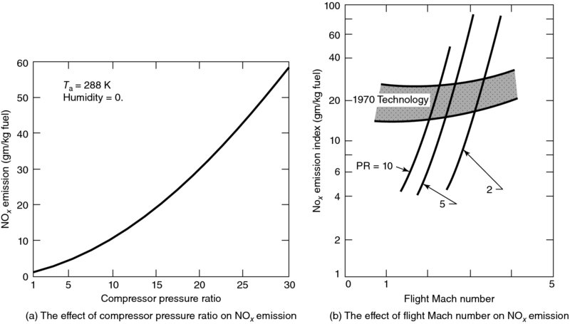
FIGURE 7.51 Impact of cycle pressure ratio (PR) on NOx emission. Source: Henderson and Blazowski 1989. Reproduced with permission from AIAA
7.7.4 Smoke
The fuel-rich regions of the primary zone in the combustor produce carbon particulates known as soot. The soot particles are then partially consumed by the high temperature gases, that is, in the intermediate and, to a lesser, extent, in the dilution zones of the combustor. Visible exhaust smoke corresponds to a threshold of soot concentration in the exhaust gases. Soot particles are primarily carbon (96% by weight), hydrogen, and some oxygen. An improved atomization of the fuel (using air-blast atomizers) and enhanced mixing intensity in the primary zone reduces the soot formation. The parameter that quantifies soot in the exhaust gases is called the smoke number, SN. Its measurement is based on passing a given volume of the exhaust gas through a filter for a specific time, then comparing the optical reflectance of the stained and the clean filter by using a photoelectric reflectometer. The procedure for aircraft gas turbine engines exhaust smoke measurements is detailed in a Society of Automotive Engineers (SAE) document – ARP 1179 (1970). The smoke number is defined as
where R is the absolute reflectance of the stained filter, and R0 is the absolute reflectance of the clean filter material.
7.7.5 Engine Emission Standards
The emission standards of the U.S. EPA (1973, 1978 and 1982) and the International Civil Aviation Organization (ICAO) (1981) define the limits on CO, UHC, NOx, and smoke production of aircraft engines near airports (Table 7.9).
![]() TABLE 7.9 EPA and ICAO Engine Emission Standards
TABLE 7.9 EPA and ICAO Engine Emission Standards
| Pollutant | EPA (1979) Standards | ICAO (1981) Standards |
| CO | 4.3 g/(kg · thrust · h) | 118 g/kN F00 |
| UHC | 0.8 g/(kg · thrust · h) | 19.6 g/kN F00 |
| NOx | 3.0 g/(kg · thrust · h) | 40 + 2(π00) g/kN F00 |
| Smoke | 19–20 | 83.6(F00)-0.274 use F00 in kN |
In the ICAO standards, the rated cycle pressure ratio π00 and the rated engine thrust F00 (in kN) are incorporated in the regulated limits.
7.7.6 Low-Emission Combustors
To combat the problems of CO and UHC production at the low engine power settings, the concept of staged combustion is introduced. This concept breaks down a conventional combustor primary zone into a pair of separately controlled combustor stages, which may be stacked (as in parallel) or in series. The stages are referred to as a pilot and a main stage, with their separate fuel injection systems. The pilot stage serves as the burner for the low power setting at peak idle combustion efficiency. The main stage is for maximum power climb and cruise condition, however, operating in a leaner mixture ratio to control NOx emissions. Complete combustion is achieved through separate fuel scheduling as well as an efficient (air-blast atomizer) fuel atomization, vaporization, and mixing in smaller volume combustors. Two concepts developed by GE-Aircraft Engines and Pratt & Whitney Aircraft are shown in Figure. 7.52.
The result of application of the double annular and Vorbix combustors to CF6–50 and JT9D-7 engines, respectively, is shown in Table 7.10 (data from Lefebvre, 1983).
![]() TABLE 7.10 Engine Emissions with Staged Combustors
TABLE 7.10 Engine Emissions with Staged Combustors
| Pollutant, g/(kg · thrust · hr · cycle) | ||||
| CO | UHC | NOx | Smoke | |
| 1979 EPA standards | 4.3 | 0.8 | 3.0 | 20 |
| production combustor | 10.8 | 4.3 | 7.7 | 13 |
| CF6–50 | ||||
| Double-annular combustor | 6.3 | 0.3 | 5.6 | 25 |
| production combustor | 10.4 | 4.8 | 6.5 | 4 |
| JT9D-7 | ||||
| Vorbix combustor | 3.2 | 0.2 | 2.7 | 30 |
The staged combustion concept is very effective in overall engine emission reduction in particular with CO and UHC, whereas NOx continues to be a challenge. To combat NOx, we should lower the flame temperature, which requires the combustor to operate at a lower equivalence ratio, of say ![]() ∼ 0.6. The problems of combustion stability and flameout accompany lean fuel–air mixtures. To achieve a stable lean mixture ratio to support a continuous combustion, a premixing, prevaporization approach has to be implemented. Both combustors that are shown in Figure 7.52 employ this concept. Also the positive impact of employing air-blast atomizers is incorporated in both combustors. However, Table 7.10 indicates higher levels of smoke are generated by the double annular and the Vorbix low-emission combustors. This reminds us of the conflict between single parameter and system optimization problems, in which different elements of the system often have opposing requirements for their optimization.
∼ 0.6. The problems of combustion stability and flameout accompany lean fuel–air mixtures. To achieve a stable lean mixture ratio to support a continuous combustion, a premixing, prevaporization approach has to be implemented. Both combustors that are shown in Figure 7.52 employ this concept. Also the positive impact of employing air-blast atomizers is incorporated in both combustors. However, Table 7.10 indicates higher levels of smoke are generated by the double annular and the Vorbix low-emission combustors. This reminds us of the conflict between single parameter and system optimization problems, in which different elements of the system often have opposing requirements for their optimization.
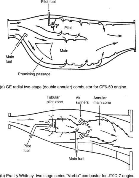
FIGURE 7.52 Examples of staged combustion for low emissions
Water injection in the combustor effectively reduces the flame temperature and has demonstrated significant NOx reduction. Figure 7.53 (from Blazowski and Henderson, 1974) shows the effect of water injection in the combustor on NOx emission reduction. We note that the ratio of water to fuel flow is ∼1 for a nearly 50% NOx reduction level. This fact eliminates the potential of using water injection at the cruise altitude to lower the NOx emissions from an aircraft gas turbine engine.

FIGURE 7.53 Water injection in the combustor reduces NOx emission. Source: Blazowski and Henderson 1974. Reproduced with permission from AIAA
Ultralow NOx combustors with premixed prevaporized gases are shown to operate at low equivalence ratios (below 0.6) when the combustor inlet temperature is increased. The application of this concept to automotive gas turbines has produced a very promising ultralow NOx emission level. The burner inlet conditions of 800 K and 5.5 atm pressures in the automotive gas turbines resemble the altitude operation (or cruise operation) of an aircraft gas turbine engine. These ultralow NOx combustor results are shown in Figure 7.54 (from Anderson, 1974).
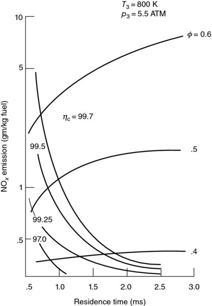
FIGURE 7.54 Effect of residence time and on NOx emission levels in ultralow NOx premixed/ prevaporized burners. Source: Anderson 1974. Courtesy of NASA
From Anderson’s results in Figure 7.54, we note that a reduced residence time, which is good for NOx production, leads to a higher level of CO and UHC emissions with an attendant combustion efficiency loss. The equivalence ratio has a large impact on NOx emissions, as seen in Figure 7.54. The NOx emission index of 0.3 g/kg-fuel seems to be the absolute minimum possible, as indicated by Anderson. To achieve these ultralow levels of the oxides of nitrogen in the exhaust emission, an increased burner inlet temperature is required. Incorporating a solid catalytic converter in an aircraft gas turbine engine burner may enable lean combustion and ultralow NOx emission but at the expense of more complexity, weight, cost, and durability. The premixed/prevaporized burners also exhibit problems with autoignition and flashback for advanced aircraft engines with high-pressure ratios. Another possibility for low NOx com-bustor development takes advantage of rich burn, which results in a reduced flame temperature, and quick quench, which allows for the combustion to be completed while the temperature of the combustion gases remain very near the combustor exit temperature. This approach is called rich burn–quick quench–lean burn and has shown promising results. These approaches are summarized in Figure 7.55, from Merkur (1996). Despite these advances, we recognize that the problem of gas turbine engine emission abatement is complex and challenging. We need to improve our understanding of the physical phenomenon in the combustor and in particular in the area of autoignition and flashback in lean combustible mixtures on the boundary of lean extinction limit.
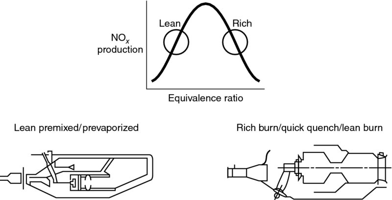
FIGURE 7.55 Approaches to a low-NOx combustor development. Source: Merkur 1996, Fig. 8, p. 8
It is instructive to compare the 1992 subsonic engine technology and the high-speed civil transport (HSCT) program goals of 2005 (from Merkur, 1996). The HSCT program is inactive at the present time (Table 7.11).
![]() TABLE 7.11 Comparison between the subsonic engine of 1992 and the design goals for the high-speed civil transport of 2005
TABLE 7.11 Comparison between the subsonic engine of 1992 and the design goals for the high-speed civil transport of 2005
| 1992 Subsonic engine | 2005 HSCT engine | |
| Equivalance ratio | ||
| Gas temperature |
3700 | |
| Liner temperature |
<1800 | |
| Liner material | Sheet or cast superalloys | Ceramic matrix composites (CMC) |
| Cooling methods | Transpiration/film | Convection |
| Environment | oxidizing | Oxidizing or reducing |
| NOx | 36–45 g/kg f | <5 g/kg f |
Source: Merkur 1996. Reproduced with permission from ASME
7.7.7 Impact of NO on the Ozone Layer
Ozone, O3, is toxic and a highly oxidizing agent, which is harmful to eyes, lungs, and other tissues. NOx production in high-temperature combustion impacts the ozone in the lower as well as upper atmosphere. In this section, the chemical processes that lead to ozone creation in the lower atmosphere and to a depletion of ozone in the stratosphere are discussed.
Lower atmosphere
Combustion at high temperature (when local combustion temperature exceeds ∼1800 K) breaks the molecular bond of N2 and O2 and causes NO to be formed, that is,
Nitric oxide reacts with the oxygen in the atmosphere to form nitrous oxide, NO2, according to
NO2 absorbs light and decomposes to
The quantity ![]() in Equation 7.140 is radiation energy with h as Plank’s constant and ν as the frequency of the electromagnetic wave. Oxygen atom is a highly reactive substance and among other reactions, it reacts with oxygen to create ozone, that is,
in Equation 7.140 is radiation energy with h as Plank’s constant and ν as the frequency of the electromagnetic wave. Oxygen atom is a highly reactive substance and among other reactions, it reacts with oxygen to create ozone, that is,
If we sum all the reactions 7.139–7.141, we get the following net result, namely,
Since NO facilitated the creation of ozone, without being consumed in the process, it is serving as a catalyst. In the lower atmosphere, nitric oxide, NO, helps generate harmful ozone in a catalyst role. The impact of NO on ozone changes as we enter the ozone layer in the stratosphere.
Upper atmosphere
The role of ozone in the upper atmosphere is to protect the earth against harmful radiation from the sun, namely, to absorb the highly energetic rays known as the ultraviolet radiation (with wavelength between 100 and 4000 Å).
The oxygen atom is highly reactive and combines with O2 to from ozone,
The photochemical cycle described by reactions 7.143 and 7.144 reactions results in no net change of the ozone concentration in stratosphere. Hence, ozone serves a stable protective role in upper atmosphere. Flight of commercial supersonic aircraft with large quantities of NO emissions (∼30 g/kg fuel) from their high-temperature engines, over extended cruise periods, and with a large fleet promises to deplete the ozone concentration levels. Again, NO appears to be a catalyst in destroying ozone in the upper atmosphere according to
By adding reactions 7.146 and 7.147 with twice the reaction in 7.145 (to get the right number of moles to cancel), we get the net photochemical reaction in the stratosphere as
Hence, ozone is depleted through a catalytic intervention of NO. The high-energy radiation absorption in stratosphere by ozone is, by and large, the source of warmth in this layer of earth’s atmosphere. Since a rise in temperature in the stratosphere with altitude is stable with respect to vertical disturbances, the ozone concentration levels should remain stable (i.e., constant) over time. A chart of ozone concentration with altitude that also depicts the best cruise altitude for the cruise Mach number of commercial aircraft is shown in Figure 7.56 (taken from Kerrebrock, 1992).
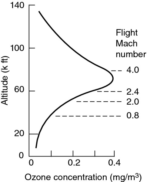
FIGURE 7.56 Profile of ozone concentration with altitude with a suitable cruise flight Mach number versus altitude superimposed. Source: Kerrebrock 1992. Fig. 4.46. Reproduced with permission from MIT Press
Now let us briefly summarize NOx formation, combustor design parameters that impact its generation, and the ozone layer.
| NOx definition: | N2O, NO, NO2 |
| Combustor reactions: | N2 + O ↔ NO + N |
| Leading to NOx: | N + O2 ↔ NO + O |
| Formation: | N + OH ↔ NO + H |
| NOx concentration: | NOx |
| Role of NOx in ozone depletion: |
O3 + hν → O2 + O where hν is the UV radiation from the sun O + O2 → O3 O + O → O2 O + O3 → 2O2 the last two reactions tend to limit the ozone concentration in the stratosphere NO + O3 → NO2 + O2 NO2 + hν → NO + O NO2 + O → NO + O2 NO is maintained, O3 destroyed |
7.8 Aviation Fuels
Aircraft flight envelope, that is, altitude Mach number, establishes the operational temperature range of the aircraft and hence its desirable fuel properties. Some of the aviation fuel properties and combustion characteristics of interest are
|
|
|
|
Let us examine the maximum skin temperature of an aircraft in cruise and compare it to the thermal characteristics of some typical aircraft fuels. The skin temperature of an aircraft is calculated through an energy balance that accounts for aerodynamic heating, radiation cooling, regenerative wall cooling, and thermal conduction. The maximum skin temperature is, however, very near stagnation temperature of flight. Figure 7.57 shows a rapid skin temperature rise with flight Mach number, assuming the cruise is in the constant-temperature layer (i.e., tropopause, between 11 and 20 km or 36–66 kft).
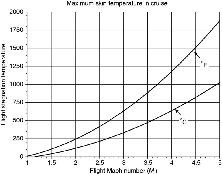
FIGURE 7.57 Skin temperature rise with flight Mach number (γ = 1.4, Tamb ≅ –70 °F or –56 °C)
At these elevated temperatures for high-speed flight, the fuel should exhibit thermal stability, which is partially addressed through its boiling point characteristics. The initial boiling point temperature begins when fuel vaporization starts. The end point is the temperature where all the fuel is vaporized. The range of the initial and end boiling points, known as the distillation curve, for several fuels is shown in Figure 7.58 (from Blazowski, 1985). The military fuels have a “JP” designation, and Jet A is the most common commercial aircraft fuel. The original gas turbine fuel was kerosene, which is used as a basis of comparison and blending with other hydrocarbon jet engine fuels. JP-4 was used primarily by the USAF and was a highly volatile fuel. A less volatile fuel, JP-5, was a gasoline–kerosene blended fuel that was used by the USN. The lower volatility of JP-5 made it more suitable for long-term storage in the ship tanks as well as the blended nature of the fuel allowed a wider availability on board a U.S. ship. The distillation curves of these two fuels may be seen in Figure 7.58, with JP-5 showing lower volatility and higher thermal stability. The low initial boiling point of JP-4 contributes to its volatility. We note that the fuels shown in Figure 7.58 are all evaporated at 100% when the fuels are heated to 250°C. At high temperatures, the fuels thermally decompose to form gum (coke deposits) and clog fuel filters, fuel injector, and the fuel pump. This limit corresponds to a flight Mach number of ∼2.6. The obvious choice for higher speed flights is the use of cryogenic fuels such as liquid methane, propane, or liquefied hydrogen. Thermal stability, flight Mach number limit, and the relative fuel cost (tentative) are shown in Figure 7.59 (from Strack, 1987).

FIGURE 7.58 Distillation curve for common jet fuels – a measure of fuel volatility. Source: Blazowski 1985. Reproduced with permission from AIAA

FIGURE 7.59 Thermal stability and relative price of aviation fuels. Source: Strack 1987. Courtesy of NASA
The specific gravity is a measure of relative liquid fuel density (relative to water at 4°C), which is lowest for gasoline among petroleum fuels. The flammability limits, flash point temperature, and spontaneous ignition temperature of various fuels are shown in a graph from Lefebvre (1983) in Figure 7.60.
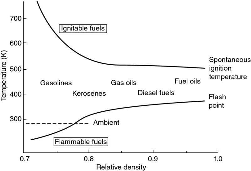
FIGURE 7.60 Ignition temperatures for petroleum fuels. Source: Lefebvre 1983. Reproduced with permission from Taylor and Francis Group LLC, a division of Informa plc
All hydrocarbon fuels have about the same heating value (nearly 18, 600 BTU/lbm or 43.3 MJ/kg) regardless of their blends. The parameter that contributes to the heat of combustion of a fuel is the hydrogen content of the fuel. For example, the percentage hydrogen content (this is the fraction of mass of the fuel molecule contributed by the hydrogen atoms) of kerosene (∼C12H26) is −15.3%, JP-4 (∼CH2.02) is at 14.5%, propane (C3H8) has 18.18%, methane (CH4) has 25%, and of course pure hydrogen is at 100% hydrogen content. It is interesting to examine the heating values of these fuels and compare them to their hydrogen content. Table 7.12 shows the impact of hydrogen content on the heat of combustion (lower heating value). The higher hydrogen content in the fuel yields a higher heat of reaction, as expected.
![]() TABLE 7.12 Hydrogen Content and Heating Value of Common Fuels
TABLE 7.12 Hydrogen Content and Heating Value of Common Fuels
| Fuel | JP-4 | Propane | Methane | Hydrogen |
| Hydrogen content | 14.5% | 18.8% | 25% | 100% |
| Lower heating value | ||||
| kcal/g | 10.39 | 11.07 | 11.95 | 28.65 |
| MJ/kg | 43.47 | 46.32 | 49.98 | 119.88 |
| BTU/lbm | 18, 703 | 19, 933 | 21, 506 | 51, 581 |
Ragozin (1962) presents a correlation between the fuel lower heating value and the percentage mass content of carbon, hydrogen, oxygen, sulfur, and water in the fuel. This useful and approximate correlation is
The dimensions of Equation 7.149 are MJ/kg. All parameters on the right-hand side are percent mass of carbon, hydrogen, oxygen, sulfur, and water in the fuel, respectively. The coefficient of hydrogen term is the largest and hence contributes the most to an increase in the fuel heating value. Also, it is interesting to note that oxygen in the fuel reduces its heating value, which is representative of all alcohol fuels (a typical alcohol fuel, ethanol, C2H5OH, has a lower heating value of ∼62% of a hydrocarbon fuel, or methanol, CH3OH, has only ∼46% of the heating value). As expected, water dissolved in the fuel also lowers the heating value of the fuel. This parameter, that is, dissolved water content in the fuel, may be controlled through proper fuel handling and storage.
Fuel viscosity is an important property that determines the pressure drop in the fuel lines and the fuel pump requirements, as well as atomization of the fuel by the fuel injection system. The lower the fuel viscosity the smaller the fuel droplets, hence faster vaporization rate and the ignition timescale. Poor atomization causes a higher fraction of UHC as well as higher CO and soot formation. On the contrary, a low viscosity fuel exhibits poor lubricity, which causes an increased fuel pump wear and reduced life. Fuel viscosity is a function of temperature and increases for a liquid fuel when temperature decreases and vice versa. At low temperatures corresponding to high altitudes, a subsonic aircraft may need an antifreeze fuel additive or employ a fuel heating system integrated with its fuel tank at the propulsion system design phase.
A liquid fuel in a tank always contains a certain quantity of fuel vapor, which exerts a pressure on the liquid. This is known as the vapor pressure of the liquid at the given temperature. For example, JP-4, a highly volatile fuel, has a very high vapor pressure of ∼0.18 atm at 38°C (or 100°F), compared with JP-5 fuel with a corresponding low vapor pressure of 0.003 atm. Although a high vapor pressure is good in a combustor and leads to better vaporization rates, it is undesirable for its lower flash point temperature. The excessive rate of vapor production in a fuel tank or a fuel line, especially at higher temperatures of supersonic flight, could lead to an unacceptable flash point fire risk. Figure 7.60 (from Lefebvre, 1983) shows the heavier fuels have a higher flash point (therefore safer) than light fuels, such as gasoline or kerosene.
Aviation fuel is a blend of different hydrocarbons with different molecular structures and different reaction tendencies. We address two such compounds, olefins and aromatics, which are found in aviation fuels. Olefins are unsaturated hydrocarbons (∼ CnH2n) that are present in aviation fuel produced in the refinery process. Aromatics (∼ CnH2n–6) are ring compounds such as benzene (C6H6) that are also present in the aircraft fuel. In the case of olefins, the gum formation tendency of these compounds makes them undesirable. The aromatics have lower hydrogen content than gasoline or kerosene, which reduces the heat of reaction of the fuel mixture. Aromatic content also increases the soot formation tendencies in the combustor, which again makes them undesirable. The volume fraction of fuel containing aromatic and olefinic compounds is included in the table of fuel properties. Table 7.13 from Blazowski (1985) presents important jet fuel properties for three widely used aircraft fuels, JP-4, JP-5 and JP-8, including, their aromatic and olefinic contents.
![]() TABLE 7.13 Important Jet Fuel Properties
TABLE 7.13 Important Jet Fuel Properties
| JP-4 | Jet A (JP-8) | JP-5 | ||||
| Property | Spec. req. | Typical value | Spec. req. | Typical value | Spec. req | Typical value |
| Vapor pressure at 38°C (100°F), atm | 0.13–0.2 | 0.18 | — | 0.007 | — | 0.003 |
| Initial boiling point (°C) | — | 60 | — | 169 | — | 182 |
| End point (°C) | — | 246 | 288 | 265 | 288 | 260 |
| Flash point (°C) | — | −25 | >49 | 52 | >63 | 65 |
| Aromatic content (% Vol) | <25 | 12 | <20 | 16 | <25 | 16 |
| Olefinic content (% Vol) | <5 | 1 | — | 1 | — | 1 |
| Saturates content (% Vol) | — | 87 | — | 83 | — | 83 |
| Net heat of combustion (cal/g) | >10, 222 | 10, 388 | >10, 222 | 10, 333 | >10, 166 | 10, 277 |
| Specific gravity | 0.751–0.802 | 0.758 | 0.755–0.830 | 0.810 | 0.788–0.845 | 0.818 |
| Approximate U.S. yearly consumption (109 gal) | 3.4 | 13.1 | 0.7 | |||
Source: Blazowski 1985. Reproduced with permission from AIAA
7.9 Alternative “Drop-In” Jet Fuels (AJFs)
Conventional aircraft engine exhaust produces a range of hazardous compounds: CO, NOx, SOx, unburned hydrocarbons (UHC) and particulate matter (soot), in addition to greenhouse gases, most notably CO2. The impact of these compounds is felt locally, through ambient air quality reductions at or near airports, and on regional or global scales, due both to the reaction and transport of compounds emitted in-flight and to the global climate impact of greenhouse gas release. For the aviation sector to evolve and grow, there must be reliable, diverse, cost effective, and environmentally sustainable energy sources. Many different feedstocks can be used to generate alternative jet fuels (AJFs), and the most economical and environmentally sustainable feedstock will likely differ by region. The description “drop-in” in AJF calls for the compatibility of these fuels with the current conventional petroleum fuels, namely in their equivalent safety and performance. The feedstocks of interest must all be second or third generation feedstocks that do not compete with the nation’s food supply. Renewable feedstocks utilize waste sources (algae grown using wastewater, lignocellulosic crop residues, municipal solid waste, wastewater, and renewable fats, oils, and grease) and existing infrastructure (woody biomass), or demonstrate promising new crops (oil-based plants, such as Jatropha curcas, and perennial grasses). For production of alternative jet fuels (AJFs) in the near term, nonconventional oil and gas supplies (oil sands, lignite coal, and natural gas) may have a lower environmental footprint than traditional jet fuels and may be easily developed with existing infrastructure. Biocoal can be produced from any carbonaceous materials and biogas can be collected from existing landfills or anaerobic digestion of waste matter from farms and wastewater treatment plants.
One key aspect of the FAA’s Destination 2025 vision calls for air travel to be environmentally sustainable. This vision is further addressed in the FAA’s March 2012 NextGen Implementation Plan, which calls for reducing aviation’s impact on the environment. The FAA has set forth an ambitious aspirational goal of having one billion gallons of drop-in jet fuel from renewable sources in use by 2018.
Alternative jet fuels (AJFs) are currently under extensive research and development to study the impact of their use in jet engines on noise pollution, engine exhaust and air quality emissions, engine deterioration and wear and complete AJF environmental benefit analysis (through life cycle assessment, LCA). Finally, the issues of supply chain development, refining infrastructure, scale production, cost and AJF qualification/certification for use in commercial aviation are some of the real-world challenges that face the aviation and energy industries.
Additional reading on AJF may be found at the FAA’s website: www.faa.gov, as well as the website of the Commercial Aviation Alternative Fuels Initiative (CAAFI) organization: www.caafi.org. An excellent overview on near-term feasibility of AJF is presented in a 2009 technical (team) report by MIT and Rand Corp. (Hileman et al., 2009). For the technical reports on the standards related to the qualification and certification of aviation fuels, the website of the American Society for Testing and Materials (ASTM), www.astm.org may be consulted.
7.10 Combustion Instability: Screech and Rumble
Acoustic waves propagate at a local speed a in a gas at rest. The acoustic waves “ride the flow, ” however, when the gas is in motion. The speed of propagation of a plane acoustic wave along the axis of a duct with a mean flow speed of u is (u + a) in the direction of the flow and (u − a) in the opposite direction. In addition, an open end of a duct or a sudden area increase/decrease in a duct causes a reflected wave to propagate back in the duct. These waves contribute to what is known as the longitudinal acoustic modes (or organ pipe modes) of a duct. We may imagine the acoustic waves propagating in the radial or in the tangential directions due to disturbances along the axis or azimuth of the duct. For example, fuel injectors in a combustor or an afterburner are placed azimuthally and flameholders in an afterburner are placed radially in the duct. Disturbances generated by these elements predominantly attain tangential and radial characteristics, respectively. The radial and tangential acoustic modes have their origin in these kinds of disturbances. Now, let us superimpose a swirl component to the mean flow and observe spinning (or tangential) modes. Add axial velocity and we get helical waves. These waves interact with each other and the sources of energy in the flow such as the mean flow or pockets of reacting gas mixtures through resonance phenomenon that leads to the growth of the disturbance wave(s) amplitude. This is similar to the dynamics of a mass-spring oscillator. The maximum energy transfer from the forcing mechanism to the driven oscillator (i.e., the mass) is found (i.e., tuned) at the resonance frequency. Nonresonant interactions are not amplified. Large-amplitude pressure waves (>10–15% of the mean) are observed in combustors at frequencies ranging from 50 to 100 Hz for longitudinal modes (called “rumble”) and as high as 5000 Hz for radial and tangential modes (called “screech”). The resonant phenomena in real systems do not have unlimited growth, however, rather they reach a limit cycle. The real systems have damping and nonlinear dynamics, which lead the oscillations to a limit cycle. Due to the large amplitudes of these high-frequency disturbances, the problem of fatigue and structural failure needs to be addressed in combustors. The reflected acoustic wave from the nozzle downstream of an afterburner couples with the combustor oscillations to create a closed-loop instability wave, known as screech.
7.10.1 Screech Damper
A Helmholtz resonator is a cavity that serves as the spring to an oscillating mass, which is contained in the neck of the cavity. The damping occurs at the natural frequency of the cavity, which is a function of the geometry of the cavity and the speed of sound. An acoustic liner composed of numerous Helmholtz resonators integrated within the liner can be designed to efficiently dampen the acoustic power near the resonant frequency of the cavity. A perforated sheet covering a honeycomb substrate is often used as an acoustic liner.
7.11 Summary
Combustion is a complex and thus challenging process. It involves chemical reactions that take place at the molecular level. The process inevitably involves fuel atomization and vaporization with subsequent mixing with an oxidizer (i.e., air in airbreathing engines) leading to a chemical reaction. We learned that the laws that govern the mixture of gases are important in a chemical reaction. To simplify our analysis, we learned and applied the concept of “chemical equilibrium” to reactions in a combustor. The wealth of experimental data on equilibrium constants allowed us to use the law of mass action to calculate the equilibrium mixture of the products of combustion. Conservation of energy principle then yielded the adiabatic flame temperature. The rate of chemical reactions identified characteristic timescales, for example, evaporation and reaction that in conjunction with the characteristic velocity scales identified a residence time, which then affected the combustor and afterburner designs.
In the combustor design section, we learned about prediffusers, flow mixing through turbulent recirculation zones that may be generated by swirl, bluff bodies, or backward-facing steps. Combustor liner cooling techniques and the use of advanced composite materials promised a lowering in the percentage coolant requirement. The nonuniformity in the combustor-exit flow was characterized by two parameters, namely, a pattern factor and a profile factor. The concern with high-altitude flameout, ignition, and relight issues were presented. Combustor pollutants in the form of UHC, CO, NOx, and greenhouse gases were discussed, and the design choices that lead to an environmentally friendly combustor were identified.
We have scratched the surface of combustion and combustor design, only. The reader should follow up this material in specialized combustion textbooks, as cited throughout this chapter. In addition, references 16, 22, 23, and 37 provide background and supplementary material and are recommended for further reading. Finally, a new area in renewable aviation fuel, i.e., Alternative Jet Fuels (AJF), was briefly introduced. AJF holds the promise of sustainable commercial aviation in the 21st Century.
References
- Adkins, R. C., “A Short Diffuser with Low Pressure Loss, ” ASME Paper, May 1974.
- Adkins, R. C., Matharu, D. S., and Yost, J. O., “The Hybrid Diffuser, ” ASME Paper 80-GT-136, 1980.
- Anderson, D. N., “Effect of Equivalence Ratio and Dwell Time on Exhaust Emissions from an Experimental Premixing Pre-vaporizing Burner, ” NASA TM-X-71592, 1974.
- Ballal, D. R. and Lefebvre, A. H., “Flame Propagation into Heterogeneous Mixtures of Fuel Droplets, Fuel Vapor and Air, ” Eighteenth International Symposium on Combustion, The Combustion Institute, Pittsburgh, 1980, pp. 321–328.
- Ballal, D. R. and Lefebvre, A. H., “Structure and Propagation of Turbulent Flames, ” Proceedings of the Royal Society of London, Series A, Vol. 344, 1975 pp. 217–234.
- Barclay, L. P., “Pressure Losses in Dump Combustors, ” AFAPL-TR-72-57 Air Force Aero-Propulsion Laboratory, Wright-Patterson AFB, OH, 1972.
- Blazowski, W. S., “Fundamentals of Combustion, ” Chapter in Aerothermodynamics of Aircraft Engine Components, Ed. Oates, G. C., AIAA Education Series, AIAA Inc. Washington, DC, 1985.
- Blazowski, W. S. and Henderson, R. E., “Aircraft Exhaust Pollution and its Effects an U.S. Air Force, ” Air Force Aero Propulsion Lab, Wright-Patterson AFB, OH, Report AFAL-TR-74-64, 1974.
- Borman, G. L. and Ragland, K. W., Combustion Engineering, McGraw-Hill, New York, 1998.
- Dugger, G. L. and Heimel, S, Flame Speeds of Methane-Air, Propane-Air and Ethylene-Air Mixtures at Low Initial Temperatures, NACA TN 2624, 1952.
- Environmental Protection Agency, Control of Air Pollution from Aircraft and Aircraft Engines, Federal Register, Vol. 38, No. 136, 1973.
- Environmental Protection Agency, Control of Air Pollution from Aircraft and Aircraft Engines, Federal Register, Vol. 43, No. 58, 1978.
- Environmental Protection Agency, Control of Air Pollution from Aircraft and Aircraft Engines, Federal Register, Vol. 47, No. 251, 1982.
- Glassman, I., Combustion, 2nd edition, Academic Press, New York, 1987.
- Gouldin, F. C., “Controlling Emissions from Gas Turbines—The Importance of Chemical Kinetics and Turbulent Mixing, ” Combustion Science and Technology, Vol. 7, 1973.
- Greenhow, V. W. and Lefebvre, A. H., “Some Application of Combustion Theory to Gas Turbine Development, ” Sixth International Symposium on Combustion, Reinhold, New York, 1957, pp. 858–869.
- Haddock, G. H., “Flame Blowoff Studies of Cylindrical Flameholders in Channeled Flow, ” Jet Propulsion Laboratory, Pasadena, California, Progress Report 3–24, May 1951.
- Henderson, R. E. and Blazowski, W. S., “Turboporpulsion Combustion Technology, ” Chapter in Aircraft Propulsion Systems Technology and Design, Ed. Oates, G. C., AIAA Education Series, AIAA Inc., Washington, DC, 1989.
- Hileman, J.I., Ortiz, D.S., Bartis, J.T., et al., “Near-Term Feasibility of Alternative Jet Fuels, ” Technical Report, Rand Corporation, Santa Monica, CA, 2009.
- Herbert, J. D., “Theoretical Analysis of Reaction Rate Controlled Systems-Part I, ” AGARD Combustion Research and Reviews, Chapter 6, 1957.
- Hill, P. G. and Peterson, C. R., Mechanics and Thermodynamics of Propulsion, 2nd edition, Addison-Wesely, Reading, Massachusetts, 1992.
- Howell, J. R. and Buckius, R. O., Fundamentals of Engineering Thermodynamics, McGraw-Hill, New York, 1987.
- Jones, R. E., Diehl, L. A., Petrash, D. A., and Grobman, J., “Results and Status of the NASA Aircraft Engine Emission Reduction Technology Programs, ” NASA TM-79009, 1978.
- Jost, W, Explosion and Combustion Processes in Gases, McGraw-Hill, New York, 1946.
- Kerrebrock, J. L., Aircraft Engines and Gas Turbines, 2nd edition, MIT Press, Cambridge, Mass., 1992.
- Kuo, K. K., Principles of Combustion, John Wiley & Sons, Inc., New York, 1986.
- Kurzke, J. and Riegler, C., “A Mixed-Flow Turbofan Afterburner Simulation for the Definition of Reheat Fuel Control laws, ” RTO-Applied Vehicle Technology panel, Symposium on Design Principles and Methods for Aircraft gas Turbine Engines, Toulouse, France, 1998.
- Lefebvre, A. H., Gas Turbine Combustion, Hemisphere Publishing Corp., New York, 1983.
- Lefebvre, A. H., “Theoretical Aspects of Gas Turbine Combustion Performance, ” College of Aeronautics Note Aero 163, Cranfield Institute of Technology, Bedford, England, 1966.
- Lefebvre, A. H. and Halls, G. A., “Some Experiences in Combustion Scaling, ” AGARD Advanced Aero-Engine Testing, AGARDograph 37, Pergamon, New York, 1959, pp. 177–204.
- Lewis, B. and von Elbe, G., Combustion Flames and Explosions of Gases, Academic Press, New York, 1961.
- Lipfert, F. W., “Correlations of Gas Turbine Emissions Data, ” ASME Paper 72-GT-60, March 1972.
- Longwell, J. E., Chenevey, W. W., and Frost, E. E., “Flame Stabilization by Baffles in a High Velocity Gas Stream, ” Third Symposium on Combustion, Flame and Explosion Phenomena, Williams and Wilkins, Baltimore, 1949, pp. 40–44.
- Merkur, R. A., “Propulsion System Considerations for Future Supersonic Transports—A Global Perspective, ”ASME Paper 96-GT-245, 1996.
- Nealy, D. A. and Reider, S. B., “Evaluation of Laminated Porous Wall Materials for Combustor Liner Cooling, ” Transaction of ASME Journal of Engineering for Power, Vol. 102, No. 2, April 1980, pp. 268–276.
- Olson, W. K., Childs, J. H., and Jonash, E. R., “The Combustion Efficiency Problem of the Turbojet at High Altitude, ” Transaction of ASME, Vol. 77, 1955.
- Pinkel, B. and Karp, I. M., “A Thermodynamic Study of the Turbojet Engine, ” NACA Report No. 891, 1947.
- Ragozin, N. A., Jet Propulsion Fuels, Pergamon, Oxford, 1962.
- Rao, K. V. L and Lefebvre, A. H., “Spontaneous Ignition Delay Times of Hydrocarbon Fuel/Air Mixtures, ” First International Combustion Specialists Symposium, Bordeaux, France, 1981, pp. 325–330.
- Rolls-Royce, The Jet Engine, Rolls-Royce, plc, Derby, England, 2005.
- Sarpkaya, T., “On Stationary and Traveling Vortex Breakdown, ” Journal of Fluid Mechanics, Vol. 45, Part 3, 1971, pp. 545–559.
- Spadaccini, L. J., “Autoignition Characteristics of Hydrocarbon Fuels at Elevated Temperatures and Pressures, ” Transactions of ASME, Journal of Engineering for Power, Vol. 99, Ser. A, No. 1, 1977, pp. 83–87 (also ASME Paper 76-GT-3, 1976).
- Spalding, D. B., Combustion and Mass Transfer, Pergamon Press Inc., New York, 1979.
- Strack, W. C., “Propulsion Challenges and Opportunities for High-Speed Transport Aircraft, ” Chapter in Aeropropulsion ’87, NASA CP-3049, November 1987.
- Strehlow, R. A., Combustion Fundamentals, McGraw-Hill, New York, 1984.
- Tacina, R. R., “Combustion Technology, ” UTSI Short Course Notes, 2000.
- Wright, F. H., “Bluff Body Flame Stabilization: Blockage Effects, ” Combustion and Flame, Vol. 3, 1959, p. 319.
- Zumdahl, S. S. and Zumdahl, S. A., Chemistry, 5th edition, Houghton Mifflin Co., Boston, 2000.
- Zukoski, E. E., “Afterburners, ” Chapter in Aerother-modynamics of Aircraft Engine Components, Ed. Oates, G. C., AIAA Education Series, AIAA Inc. Washington, DC, 1985.
- Zukoski, E. E. and Marble, F. E., “The Role of Wake Transition in the Process of Flame Stabilization on Bluff Bodies, Combustion Researches and Reviews, 1955, Butterworths Scientific Publications, London, 1955.
- Zukoski, E. E. and Marble, F. E., “Experiments Concerning the Mechanism of Flame Blowoff from Bluff Bodies, Proceedings of the Gas Dynamics Symposium on Aerothermochemistry, Northwestern University Press, Evanston, Illinois, 1955.
Problems
- 7.1 A mixture of gases contains 44 kg of CO2, 112 kg of N2, and 32 kg of O2 at a mixture temperature of Tm = 287 K and the mixture pressure is pm = 1 bar.
Calculate
- number of moles of carbon dioxide, nitrogen, and oxygen
- mole fraction of carbon dioxide
- partial pressure of constituent gases, i.e., CO2, N2, and O2
- mixture molecular weight MWm
- volume fraction of the constituent gases
- 7.2 Write the chemical reaction for the combustion of hydrogen, H2, and air then calculate the stoichiometric fuel-to-air ratio fstoich.
- 7.3 A gas is a mixture of 22% O2, 33% N2, and 45% CO2 by volume. Calculate
- the mole fraction of the constituents in the mixture
- the mixture molecular weight MWm
- 7.4 Write the chemical reaction for the complete combustion of JP-4 and air. JP-4 has the formula CH1.93. Also, calculate the stoichiometric fuel-to-air ratio for this blended jet fuel.
- 7.5 Calculate the lower and higher heating values of octane, C8H18, in the stoichiometric chemical reaction with oxygen at a reference temperature of 298.16 K and the pressure of 1 bar.

- 7.6 Establish the higher and lower heating values of octane, C8H18, by considering the stoichiometric reaction in air at a reference temperature of 298.16 K and at 1 bar pressure.
Compare your answer to Problem 7.5 and explain.
- 7.7 Adiabatic flame temperature associated with the combustion of a fuel in air depends on the temperature and pressure of air. Figure 7.6 shows the adiabatic flame temperature of Jet-A fuel in air with initial temperature of 800 K and initial pressure of 25 atm.
- What is the stoichiometric flame temperature of JP-A if the initial air temperature was 1000 K at 25 atm pressure?
- What is the stoichiometric flame temperature of Jet-A if the initial pressure of air was 1 atm and the initial temperature remained at 800 K?
- 7.8 Consider burning methane (CH4) with 110% theoretical air. Calculate the equivalence ratio for this reaction. Assume that the nitrogen and the excess oxygen do not dissociate and/or chemically react to form new compounds.
- 7.9 One mole of octane is burned with 120% theoretical air. Assuming that the octane and air enter the combustion chamber at 25°C and the excess oxygen and nitrogen in the reaction will not dissociate, calculate
- the fuel–air ratio
- the equivalence ratio
- the adiabatic flame temperature Taf
Assume

- 7.10 One mole of oxygen, O2(g), is heated to 4000 K at the pressure of pm. A fraction of the oxygen dissociates to oxygen atoms according to

Assuming a state of equilibrium is reached in the mixture, calculate
- mole fraction of O2 at equilibrium when pm is 1 atm.
- mole fraction of O2 at equilibrium when pm is 10 atm.
Assume the equilibrium constant for the reaction

is Kp = 2.19 atm at the temperature of 4000 K. Explain the effect of pressure on dissociation.
- 7.11 One mole of gaseous hydrogen is heated to 3000 K at the pressure of pm. Assuming a fraction of the hydrogen dissociates upon heating into atomic hydrogen, i.e.,

calculate the mole fraction of hydrogen, H2, in the equilibrium mixture for pm = 1 atm and pm = 10 atm. Does higher mixture pressure inhibit or promote the dissociation of hydrogen?
You may find the equilibrium constant Kp for the following stoichiometric reaction

at 3000 K from Table 7.3.
- 7.12 Mass flow rate (combined fuel and air) into a reactor of volume 2.35 ft3 is 100 lbm/s. The equivalence ratio is 0.6. Use the combustor loading parameter (CLP)

and the combustor stability loop (Figure 7.22) to establish the range of reactor pressure that leads to a stable combustion. Note that the scale is logarithmic.
- 7.13 Combustion involves many timescales. For example, a flammable mixture of fuel and air (under a spontaneous ignition temperature condition) experiences an ignition delay time ti. The elements contributing to the ignition delay time are the fuel droplet evaporation time and a reaction timescales. The ignition delay results of the combustion of two hydrocarbon fuels at 10 atm of pressure are shown in Figure 7.24. Graph an estimated ignition delay time for the same fuels but at the pressure of 30 atm by assuming pressure dependence for the reaction timescale is For a first-order approximation, you may neglect the evaporation time dependence on the mixture pressure.
- 1
 p
p - 1p1.5
- 1
- 7.14 An afterburner uses flameholders with a drag coefficient of CD = 0.5, based on the afterburner cross-sectional area. The inlet Mach number to the afterburner is Mi = 0.2, with γi = 1.33. The heat release due to combustion in the afterburner is q/cpiTti = 2.0. The exhaust gas in the wet mode has a lower ratio of specific heats, namely, γe = 1.30. Calculate
Dry mode
- exit Mach number Me
- total pressure loss as a percentage of inlet total pressure
Wet mode
- exit Mach number Me
- total pressure loss as a percentage of inlet total pressure
- 7.15 A combustion chamber uses a prediffuser with a sudden area expansion (known as a dump diffuser) to decelerate the flow of air (γ = 1.4) before entering the combustor. Assuming the inlet Mach number to the dump diffuser is M1 = 0.5, the area ratio of the dump diffuser is A2A1 = 2.0, calculate
- exit Mach number M2
- the ratio of total pressures, i.e., pt2pt1
- 7.16 Calculate the higher and lower heating values of methyl alcohol, CH3OH, and methane, CH4, by considering the following reactions at the reference temperature of 298.16 K and at 1 bar pressure.
Note that the products of combustion for both reactions are the same. Explain the difference between the heating values of these two fuels that are seemingly so similar.
- 7.17 Calculate the lower and higher heating values of propane, C3H8, in the following chemical reaction at a reference temperature of 298.16 K and the pressure of 1 bar.

- 7.18 Gaseous hydrogen and air enter an adiabatic combustion chamber at a temperature of 298.16 K (the reference temperature) and pressure of 1 bar.

Assuming the average molar specific heats of the products are
Calculate
- fuel-to-air ratio
- the adiabatic flame temperature Taf
- 7.19 Stoichiometric flame temperature for the combustion of methane in oxygen at 1 atm pressure and at reference temperature of 298 K is listed as 3030 K in Table 7.4. The combustion of methane in air would produce the stoichiometric flame temperature of 2210 K. Explain the difference.
- 7.20 An annular combustor utilizes a dump prediffuser, as shown. Calculate
- the diffuser area ratio A2A1
- the total pressure loss Δptpt1
- exit Mach number M2
Assume the inlet Mach number is M1 = 0.4 and γ = 1.4.
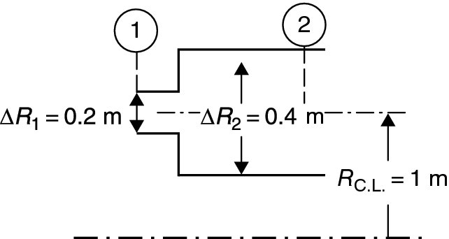
- the diffuser area ratio A2
- 7.21 Consider a coaxial dump diffuser with area ratio A2A1. Assuming that the static pressure acting on the sudden expansion wall pw is the same as the inlet static pressure p1 and wall friction may be neglected, apply the conservation principles to show that
in the limit of incompressible fluid.
Assume the flow is uniform at the exit.
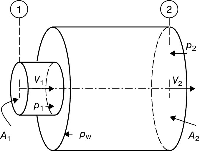
- 7.22 Take two parallel streams with initial speeds of 20 and 30 m/s, as shown.
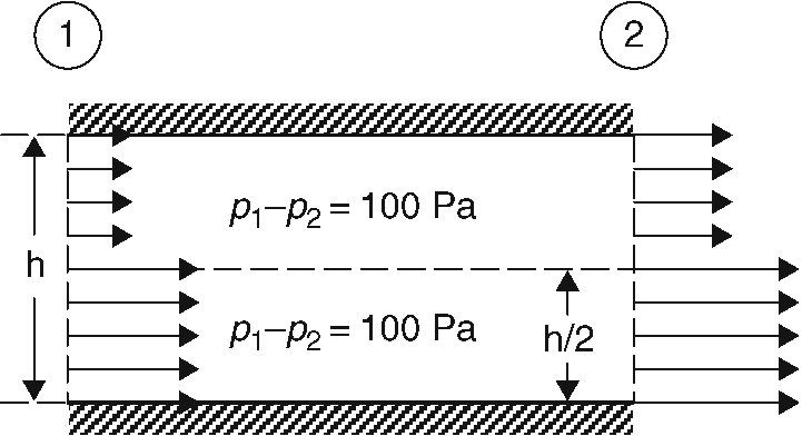
Assuming the two streams do not mix and thus remain parallel, calculate
- the initial distortion level
- the final speed of both streams
-
the final distortion level
Here, we define the distortion level as
 where
where  is the area-averaged u.
Assume the fluid density is constant at 1 kg/m3.
Why did the distortion level decrease in this case?
- Repeat this problem with a static pressure rise p1 − p2 = −100 Pa, instead of a static pressure drop. Explain the distortion level behavior.
- 7.23 The effect of flammability limit on gasoline–air mixture as a function of combustion pressure is presented in Figure 7.11. First, what is the lowest pressure that combustion is possible? Second, at combustion pressure of 1.8 psia, what are the equivalence ratios corresponding to the flammability limits?
- 7.24 We model an afterburner as a constant-area duct with a series of bluff bodies in the stream with a known drag coefficient. Assuming the following inlet conditions for dry mode
Inlet Mach number Mi = 0.3
γi = γe = 1.33 and cpi = cpe
flameholder drag coefficient CD = 0.5
Calculate
- static pressure ratio pepi
- exit Mach number Me
- static temperature ratio TeTi
- total pressure ratio ptepti
- static pressure ratio pe
- 7.25 The afterburner in Problem 7.24 operates in “wet mode.” Assuming the nondimensional heat release q/cpiTti = 1.0 and γe = 1.25 in wet mode, calculate
- total pressure ratio in the wet mode
- exit Mach number in the wet mode
- 7.26 Atmospheric ozone is depleted through catalytic intervention of nitric oxide, NO. NO emissions in the upper atmosphere are estimated to be ∼30 g/kg fuel from high-temperature engines, overextended cruise periods. A supersonic transport carries 50, 000 kg of fuel at takeoff. Assuming 90% of the fuel is consumed during cruise calculate the amount of nitric oxide emissions for a round trip flight. Now, multiply that by 360 round trips per year to estimate the (NO) pollution (of one aircraft) per year. Finally, what is the environmental impact ofa fleet of 100 aircraft?
- 7.27 Emission index (EI) of carbon monoxide and unburned hydrocarbons at idle power is shown in Figure 7.49. Assuming that the combustor inlet temperature at idle power is 425 K, read an average value of the emission index for carbon monoxide and unburned hydrocarbons from the graph. Then, calculate the combustion inefficiency from

and compare the combustion efficiency ηb at idle setting to EPA standards (of 99%).
- 7.28 Carbon monoxide is a byproduct of incomplete combustion of hydrocarbon fuels and is considered to be a pollutant. It is also a fuel capable of reacting with air to produce an adiabatic flame temperature of ∼2400 K at the pressure of 1 atm (Table 7.4). The stoichiometric combustion of carbon monoxide and air may be described by the following reaction:

Use conservation of energy principles applied to the above stoichiometric reaction to show that the adiabatic flame temperature of carbon monoxide is indeed ∼2400 K in a reaction with air at 1 atmospheric pressure.
You may use Table 7.1 for standard heats of formation and Table 7.2 for molar specific heats of various gases. Assume the reactants enter the combustion chamber at Tf = 298.16 K.
- 7.29 Air composition at room temperature is approximated by 21% O2 and 79% N2 by volume, or by mole fractions, i.e., one mole of air is composed of

Strong shocks are, however, formed when aircraft fly at supersonic/hypersonic Mach numbers. The composition of air thus changes as a sudden compression is encountered through a shock. At 6000 K and one atmospheric pressure, one mole of air assumes the following equilibrium composition:

Calculate
- the molecular weight of air in the new mixture, MWm, in kg/kmol
- the fuel-to-air ratio for the stoichiometric combustion of hydrogen in air (at 6000 K)
- 7.30 Unburned hydrocarbons, UHC, and nitric oxide, NO, are formed as products of combustion in aircraft gas turbine engines. They lead to burner inefficiency, as they still possess heating value. Consider the combustion of NO, at reference temperature and pressure, to estimate the heating value of NO, in the following stoichiometric reaction:

- 7.31 Combustion of gaseous methane with dry air is shown as:

Assuming the air entered at reference temperature of Tf = 298.16 K and pressure of 1 bar, calculate the
- fuel-to-air ratio, f
- equivalence ratio,
- adiabatic flame temperature, Taf, in K
Use the chemical properties shown in the box.


- 7.32 Write the stoichiometric combustion of methanol (CH3OH) in (dry) theoretical air. If the lower heating value, LHV, of methanol is 21.2 MJ/kg, calculate its higher heating value, HHV.
- 7.33 Calculate the adiabatic flame temperature in the following reaction of octane in dry air at reference temperature (Tf = 298.16 K) and pressure (1 bar),

Assume the average molar specific heats of the chemical compounds at constant pressure are:
The standard heats of formation in this reaction are:
- 7.34 In the combustion of gaseous hydrogen and gaseous oxygen, as described by

the reactants entered the combustion chamber at T1 = 298.16 K and pressure of 1 atm. Assume:

Calculate the
- heat of reaction, QR, in kJ
- lower heating value, LHV, in kJ/kg
- adiabatic flame temperature, Taf, in K
- 7.35 Consider the combustion of butane and air according to

Calculate the
- fuel-to-air ratio, f
- equivalence ratio, ϕ, for this reaction
- 7.36 Lean combustion of liquid n-decane (from the kerosene family) and air at a reference temperature of Tf = 298.16 K and pressure of 1 bar is approximated by the following chemical reaction:

Assuming the standard heats of formation in this reaction are:
and average molar specific heats at constant pressure are:
Calculate
- the fuel-to-air ratio, f, for this reaction
- write the stoichiometric reaction for this fuel in air
- the equivalence ratio,
- the adiabatic flame temperature, Taf, in K in the first reaction
- the Lower Heating Value (LHV) of this fuel, in kJ/kg, in stoichiometric combustion in oxygen
- 7.37 Write the stoichiometric combustion of propane (C3H8) in theoretical air. If the lower heating value, LHV, of propane is 46.32 MJ/kg, calculate its higher heating value, HHV.
- 7.38 Calculate the adiabatic flame temperature in the combustion reaction of octane in air at reference temperature (Tf = 298.16 K) and pressure (1 bar),
You may assume the average molar specific heats of the compounds at constant pressure are:

The standard heats of formation in this reaction are listed in Table 6.1 in the book as:

- 7.39 Consider the flow in an afterburner, in dry mode, as shown. The flow upstream of the flameholder, i.e., the afterburner inlet, is characterized by:

Assuming the flameholder drag coefficient is CD = 1.0, which is based on the duct cross-sectional area, and the flow is adiabatic, calculate
- the duct cross sectional area, A1, in m2
- flameholder drag, Dflameholder, in kN
- static pressure in station 2, where M2 = 0.371, γ2 = γ1 = 1.33 and wall friction drag coefficient is neglected (i.e., Cfw = 0) as shown
- static temperature in station 2, T2, in K
- 7.40 Consider the stoichiometric combustion of one mole of octane in dry air, where the carbon in fuel is completely oxidized to form eight moles of CO2 in the products, as shown in the following reaction
Assuming the reactants entered the combustion chamber at reference temperature of 298.16 K and combustion takes place at reference pressure of 1 bar, calculate:
- adiabatic flame temperature, Taf (K), of octane in the above reaction
Now, consider the same reactants at the same entrance condition and pressure engage in combustion that produces seven moles of carbon dioxide and one mole of carbon monoxide in the products of combustion, following
Calculate
- the adiabatic flame temperature of octane in the second reaction
- compare the two adiabatic flame temperatures and briefly comment on the cause for the difference


- 7.41 The chemical reaction of gaseous octane in air reaches an equilibrium state in a combustor that is described by:
Assuming the reactants entered the combustor at the reference temperature (298.16 K) and pressure (1 atm), calculate the
- fuel-to-air ratio, f
- equivalence ratio, ϕ
- adiabatic flame temperature, Taf, in K, at the combustor exit
Assume the molar specific heats of the products are:

- 7.42 Consider the stoichiometric combustion of gaseous ethyl alcohol (or ethanol) in air, as shown:
Assuming the reactants entered the combustion chamber at reference temperature of 298.16 K and combustion takes place at reference pressure of 1 bar, calculate the
- adiabatic flame temperature, Taf, in K, of ethanol in stoichiometric combustion
- lower heating value (LHV) of ethanol in kJ/kg
- higher heating value (HHV) of ethanol in kJ/kg


- 7.43 Write the stoichiometric combustion of C6H6 with (dry) theoretical air.
- 7.44 Consider the stoichiometric combustion of Jet-A fuel, C12H23, in (dry) air.
- Write the chemical reaction between Jet-A fuel and air in stoichiometric combustion
- Calculate stoichiometric fuel-to-air ratio in this reaction