
CHAPTER 9
Centrifugal Compressor Aerodynamics
9.1 Introduction

CFD results shown in a centrifugal compressor. Source: Courtesy of NASA
Centrifugal compressors belong to the general category of turbomachines. The flow may enter a centrifugal compressor in the axial direction. The rotor, which is known as the impeller, imparts energy to the fluid by the rotation of its aerodynamic surfaces (i.e., blades or impeller vanes) that are highly curved and twisted. The initial curvature and twist in the impeller, known as the inducer section, has the function of meeting the incoming flow at its relative flow angle. The second function of the inducer is to turn the relative flow toward the axial direction before it begins its journey in the radial direction. The third function of the inducer is to increase the fluid static pressure in the passage by decelerating the gas. The inducer exit flow is then further decelerated radially outward, by virtue of centrifugal force acting on the fluid in the spinning impeller (vaned) passages. Since the pressure rise in this type of configuration is primarily produced by centrifugal compression/force, this kind of turbomachinery is known as a centrifugal compressor. In contrast to axial-flow compressors where the flow deviation in the radial direction is negligible, the principle of operation of the centrifugal compressor is based on large radial shift between the inlet and exit of the impeller (Figure 9.1). Since the impeller exit radius is by design much larger then the impeller inlet radius, the centrifugal compressors have a lower mass flow rate per frontal area than the axial-flow compressors. A low mass flow per frontal area is of critical concern to aircraft propulsion system designers, since it translates into an increased drag count. However, in low-speed applications where the drag penalty is less significant, centrifugal compressors offer the advantage of high-pressure ratio per stage and robustness of construction that is less prone to structural failure. There are other applications for small gas generators on board aircraft that are suitable for centrifugal compressor application. For example, APUs (auxiliary power units) are used to start the engines and provide power to aircraft, which are entirely embedded in the fuselage; therefore, there are no concerns of external drag penalties for their use. Industrial and automotive turbocharging applications also use centrifugal compressors.

 FIGURE 9.1 Schematic drawing of a first (left) and a second stage (right) centrifugal compressor
The radially pumped flow from the impeller first needs to be decelerated through a radial and vaned diffuser, and then it needs to turn back toward the axis of rotation for either the next compressor stage or the combustion chamber. Since any ducting that involves turns is a source of (total pressure) loss, multistage centrifugal compressors are considered cumbersome (and with lower efficiency) as compared with axial-flow compressors. However, the total pressure ratio of a single-stage centrifugal compressor may be as high as 10–12, whereas an axial-flow compressor stage produces a high of ∼1.6–2.0 in advanced transonic fan stages.
9.2 Centrifugal Compressors
A centrifugal compressor is a robust mechanical compression system that pumps the gas from primarily an axial inlet condition to a radial exit direction. The elements of a centrifugal compressor rotor, known as the impeller, are shown in Figure 9.2.
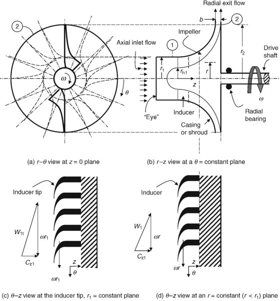
FIGURE 9.2 Definition sketch of a centrifugal compressor impeller with an inducer
The inlet section of an impeller is called the inducer, which is turned in the direction of impeller rotation to meet the flow at a small incidence angle. The radial displacement of the fluid in the inducer is small but the flow turning is rather large. The inducer turns the fluid from the inlet relative flow direction β1 to the axial direction. The static pressure rise in the inducer is due to the conversion of relative swirl kinetic energy in a curved diffuser. The outer portion of the impeller is responsible for turning the flow in the radial direction and accelerating the fluid in the tangential direction. The torque acting on the fluid causes the angular momentum to change across the rotor blade following Euler turbine equation:
As in the axial-flow compressors, we note that the torque acting on the fluid is positive across the rotor (as r2Cθ2 > r1Cθ1) and thus the rotor torque being equal and opposite is negative. Then multiplying the rotor torque with the angular speed of the shaft, ω, we get a negative shaft power that is delivered to the rotor. This is consistent with the thermodynamic convention employed in the first law that considers the work done on the surrounding as positive. Therefore, the work done by the surrounding (as needed by compressors) is then negative. The torque acting on the fluid crossing the stator, as in the axial-flow compressors, is negative. Therefore, the stator vanes experience a positive torque. There will not be any contribution to the fluid power by the stator blades as they are stationary and thus perform no work on the medium. The shaft power delivered to the fluid is converted into total enthalpy rise according to
The rotor total temperature ratio is deduced from Equation 9.1, that is,

In Equation 9.1, the impeller radius ratio (r1/r2) is small, which makes the second term in the bracket negligible compared with the first term. In addition, either due to a lack of inlet guide vanes, which results in Cθ1 to be identically zero, or the fact that Cθ2 ![]() Cθ1 in a centrifugal compressor, we often neglect the second term in the bracket in Equation 9.2 in favor of the first term, that is,
Cθ1 in a centrifugal compressor, we often neglect the second term in the bracket in Equation 9.2 in favor of the first term, that is,

However, note that we do not have to neglect the second term in Equation 9.2, as the inlet swirl Cθ1 may be treated as a known input to the problem.
There are three types of impeller geometry:
- Radial impeller
- Forward-leaning impeller
- Backward-leaning (or backswept) impeller.
A schematic drawing of impeller geometries and their corresponding velocity triangles are shown in Figure 9.3.

FIGURE 9.3 Definition sketch of the impeller blade shapes, flow angles, ideal velocity triangles at the impeller exit, and the phenomenon of slip
The radial impeller offers radial passages to accelerate the fluid in the rotor and ideally attain a radial exit flow. The forward-leaning impeller geometry accelerates the fluid in a spiral passage leaning in the direction of the rotor rotation. The backswept impeller is composed of spiral passages that direct the relative flow in the opposite direction to rotor rotation. The geometry of the impeller dictates the exit flow angle β2 and thus strongly impacts the magnitude of the exit swirl velocity Cθ2. The three types of impeller geometry are shown in Figure 9.3, with the flow angles at the impeller exit now measured with respect to the radial direction, as shown. The velocity triangles at the impeller exit show that the absolute swirl is increased when the impeller geometry is forward leaning (with β2 < 0). For the case of the straight radial impeller, the exit absolute swirl should theoretically be the same as the wheel speed U2. The backward-leaning or backswept impeller geometry turns the relative flow in the opposite direction to the wheel rotation (with β2 > 0), therefore the absolute swirl in the exit plane is reduced. All these arguments are the results of simple interpretation of the velocity triangles (Figure 9.3).
The Euler turbine equation suggests that the forward-leaning blades produce the highest total enthalpy rise and, hence, absorb the maximum shaft power. The impeller exit Mach number is the highest of the three designs and thus limits the static pressure recovery and efficiency of the radial diffuser. Also, the blades are under severe structural loads in bending due to their curvature. Similarly, the blades of a backward-leaning impeller are under high structural loading and the shaft power absorption is reduced. The exit Mach number of the backward-leaning impeller is the lowest of the three designs and will be explored as an alternative to radial impeller design. The lower exit Mach number of the backward-leaning impeller is attractive in achieving higher efficiency diffusion in the radial diffuser. The optimum geometry from structural standpoint seems to be the straight radial impeller with good power absorption, acceptable stability characteristics, and a low level of structural loading (in bending) due to purely radial design. However, the pressure rise in the compressor increases with the wheel speed, hence a backward-leaning impeller design could operate at higher UT once the structural design issues are resolved.
In the rotor frame of reference, the flow in the impeller is primarily in the radial direction, which bends in the opposite direction to the wheel rotation due to a Coriolis force, that is, ∝2ω Wr. The presence of tangential pressure gradients in addition to the Coriolis effect combine to create a countercirculation in impeller blade passages toward the trailing edge. The counterrotation in the impeller exit flow causes a reduction in the absolute swirl, therefore a reduction in the power absorption and thus leads to a reduced pressure ratio. This phenomenon is known as slip in centrifugal compressors. An example of the slip in a straight radial impeller is shown in Figure 9.3d. The other two examples of impeller configurations, that is, the forward- and the backward-leaning types, are subject to the phenomenon of slip in their respective passages. We define a slip factor for radial impellers as the ratio of absolute swirl to the exit wheel speed, which represents the ideal swirl had the fluid attained the same tangential velocity as the disk, namely,
Hence, the total temperature rise across the straight radial impeller is related to the wheel speed and the slip factor ![]() following the Euler turbine equation, that is,
following the Euler turbine equation, that is,

From Equation 9.5a, the impeller loading coefficient ![]() gives a simple expression for the radial impeller, which is independent of mass flow rate, assuming constant slip factor, that is,
gives a simple expression for the radial impeller, which is independent of mass flow rate, assuming constant slip factor, that is,
In general, the slip factor is defined as
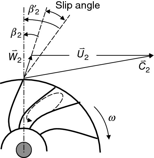
where the ideal exit swirl is calculated based on the impeller blade exit angle β′2, and the actual exit swirl is based on the actual exit flow angle β2. Figure 9.4 shows a definition sketch of these angles for the backward and forward-leaning impellers.

FIGURE 9.4 Definition sketch for the slip flow in a backswept and forward-leaning impeller
If we adopt the sign convention that the impeller exit angle is measured from the vane position to the radial direction and is positive in the direction of the rotor rotation, we note that a backswept impeller has a positive β′2 and a forward-leaning impeller has a negative vane exit angle β′2. With a similar sign convention for the exit flow angle, we may write the ideal and actual exit swirl velocities in terms of the impeller exit angle β′2, flow angle β2 as
From Equation. 9.7a, we note that a backswept impeller, with a positive exit vane angle, reduces the absolute (ideal) swirl, whereas a forward-leaning impeller with a negative vane angle increases the exit absolute swirl. Similar argument can be made regarding the exit swirl velocity in the actual flow as described in Equation. 9.7b. We define the slip factor as the ratio of actual to the ideal exit swirl as
The impeller specific work and the loading are written as

We may graph Equation 9.7b, that is, the variation of the nondimensional work, or the impeller-loading coefficient ![]() , with flow coefficient Cr2/U2 (which is similar to Cz/U in axial-flow compressors), for different impellers. Figure 9.5 shows the impeller loading variation with flow coefficient for the three impeller types (with a constant slip factor
, with flow coefficient Cr2/U2 (which is similar to Cz/U in axial-flow compressors), for different impellers. Figure 9.5 shows the impeller loading variation with flow coefficient for the three impeller types (with a constant slip factor ![]() ).
).

FIGURE 9.5 Centrifugal compressor impeller loading variation with flow coefficient or mass flow rate
There are several correlations between the slip factor ![]() and the number of the impeller vanes N in radial impellers, which are proposed by Stodola (1927), Busemann (1928), and Stanitz–Ellis (1949). The Stanitz–Ellis model, which is similar to Stodola’s, is considered a reasonable approximation for the slip factor in straight-radial impellers (and a first-order approximation for other impeller types),
and the number of the impeller vanes N in radial impellers, which are proposed by Stodola (1927), Busemann (1928), and Stanitz–Ellis (1949). The Stanitz–Ellis model, which is similar to Stodola’s, is considered a reasonable approximation for the slip factor in straight-radial impellers (and a first-order approximation for other impeller types),
A 20-bladed impeller, for example, will experience a slip factor of ∼0.9 in its energy transfer to the fluid. For radial impellers, the slip factor (as expressed in Equation 9.10) is independent of the mass flow rate. However, slip factor in reality is a function of the mass flow rate for all three configurations, that is, radial, forward- and backward-leaning impellers. Increasing the number of the impeller blades reduces the effect of slip, which in turn increases the weight. To achieve the effect of higher blade count without investing heavily in the system weight increase, a compromise solution is found by incorporating splitter vanes in the outer half of an impeller disk. The presence of splitter vanes acts as an inhibitor of counterswirl produced in the outer portion of an impeller disk and possible reduction of flow separation in the impeller. Figure 9.6 shows the splitter vanes concept in a centrifugal turbomachinery. A parallel argument in the creation of slip is worthy of discussion. The flow at the exit of the inducer is turned parallel to the axis and is starting its journey in the radial direction. Therefore, the rotor flow is purely radial at the exit of the inducer. This resembles a source flow, which is irrotational. For the flow to remain irrotational (in the absence of external forces, i.e., in rotor frame of reference), counter eddies of the same angular speed need to be set up in the impeller blade passages. The counter eddies thus lead to an exit flow that is rotated in the opposite direction to the wheel rotation, by an angle known as the slip angle.
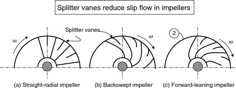
FIGURE 9.6 Schematic drawing of splitter vanes on the impeller disk of a centrifugal compressor
The stage total temperature ratio is the same as the impeller total temperature ratio, since the stationary blades are adiabatic and do no work on the fluid; therefore, we may write Equation 9.3 as
The stagnation speed of sound at the inlet condition is at1 in Equation 9.11. The ratio of wheel speed at the impeller exit to the stagnation speed of sound at the inlet is a non-dimensional parameter that is called the Mach index ΠM in the centrifugal compressor literature. In terms of the Mach index, we may write the stage total temperature ratio for a straight-radial impeller with zero preswirl as
Upon closer examination of this parameter, that is, Mach index, we note that it is directly proportional to the impeller tangential Mach number at the exit and inversely proportional to the axial Mach number at the inlet of the compressor. This relation is shown in Equation 9.13.

where ![]()

FIGURE 9.7 Comparison between the Mach index and impeller tip Mach number MT2
The impeller total pressure ratio is related to the impeller total temperature ratio via polytropic efficiency according to

where we replaced the Mach index with the tip tangential Mach number. Now, let us graph this equation for different tip tangential Mach numbers. Figure 9.8 shows the functional dependence of pressure ratio and tip Mach number. We note an exponential growth of the impeller total pressure ratio with the tangential Mach number at the impeller tip. There are two limitations to the exponential growth performance of centrifugal compressors with tip tangential Mach number depicted in Figure 9.8. One limiting factor is due to excessive centrifugal stresses and the structural loads; the second limiting factor is due to a drop in efficiency of the diffusion process in the radial diffuser at high inlet supersonic Mach numbers. To tackle the structural problem, a high strength-to-weight ratio material is desirable for the rotor application. Titanium alloys are thus suitable, and the lighter, lower cost aluminum is still considered a material of choice for small centrifugal compressor applications. The impeller rim speed of ∼1700 ft/s (or ∼520 m/s) represents the state-of-the art in centrifugal compressors. The corresponding tangential rim Mach number defined as the ratio of rim speed to the inlet speed of sound a1 at standard sea level inlet condition, that is, a1 of 1100 ft/s or 340 m/s, is limited to MT2 ∼ 1.55. From the three possible impeller geometries, the forward-leaning design would create a higher exit Mach number than the rim tangential Mach number, based on the velocity triangle depicted in Figure 9.3a. Therefore the inlet Mach number to the diffuser will be even higher than 1.55, based on the inlet speed of sound (a1). The straight-radial impeller would roughly achieve the same diffuser inlet Mach number as the impeller tangential rim Mach number. Note that the radial flow Mach number is small compared with a supersonic tip. To reduce the diffuser inlet Mach number to lower than 1.55 (based on a1), we may lean the impeller blades backward, known as backsweep. The main disadvantage of curved impellers, that is, both the forward- and backward-leaning types, is in their higher (bending) stress levels than the radial vanes. The curved impellers experience large bending stresses due to the centrifugal force, whereas the radial impellers theoretically experience no bending stresses due to centrifugal loads. The higher cost of manufacturing attributed to curved impellers is considered their second disadvantage as compared with straight-radial impellers. Despite higher manufacturing costs and higher stresses, the trend is to maximize the wheel speed for efficient centrifugal compression while reducing the diffuser entrance Mach number by backward-leaning the impeller blades. The backswept impellers of ∼45° exit sweep represent the state of the art in high performance centrifugal compressors.

FIGURE 9.8 Variation of impeller pressure ratio with tip tangential Mach number (based on the inlet speed of sound, a1) for a straight-radial impeller with slip factor  = 0.9
= 0.9
So far we have referenced impeller exit velocity components to the inlet speed of sound. The behavior of actual flow in the diffuser depends, however, on the Mach number based on the local speed of sound at the impeller exit, a2. The Euler turbine equation applied to an impeller with zero inlet swirl (or preswirl) is the starting point of our calculation of T2, or a2, that is,
From the definition of slip factor, Equation 9.8, we will substitute for the ratio of exit absolute swirl to the wheel speed in the above equation to get

Now, the total temperature ratio may be related to the static temperatures and the fluid kinetic energy following the definition of total enthalpy, that is,

The contribution of kinetic energy at the entrance to the centrifugal compressor may be neglected in favor of the static temperature and thus Equation 9.17 may be approximated as
The right-hand side of Equation 9.18 may be simplified if we replace the absolute kinetic energy with the swirl kinetic energy, which essentially neglects small contribution of the exit radial kinetic energy. We may solve for the static temperature ratio as
By substituting for the total temperature ratio from Equation 9.16 and the ratio of exit swirl to the wheel speed from Equation 9.8, we get the impeller static temperature ratio as

The parameters on the right-hand side of Equation 9.20 are all nondimensional design parameters. In its simplest form, where we set radial velocity nearly equal to zero for curved impellers or in the case of straight-radial blades, β′2 = 0, and neglect slip, that is, ![]() = 1, the static temperature ratio reduces to
= 1, the static temperature ratio reduces to
Since the total temperature through the stator remains constant, the impeller static temperature rise is half of the stage total temperature rise, which for low speed at the exit of the diffuser becomes one half of the stage static temperature rise (T3/T1 – 1). Therefore, under these conditions, the rotor and the stator produce the same static temperature rise, or what was called a 50% degree of reaction. The ratio of the speed of sound at the impeller exit to the inlet speed of sound is the square root of the static temperature ratio as

From Equation 9.14, we may substitute for the Mach index in terms of the wheel tangential Mach number MT2 and the inlet Mach number M1 to write the ratio of the speeds of sound across the impeller as

We may now graph this expression to examine the rise of speed of sound across the impeller. Figure 9.9 shows the ratio of speed of sound across the impeller.
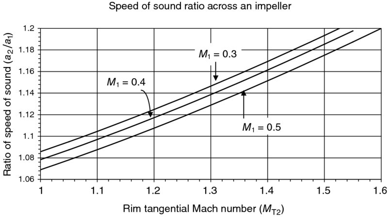
FIGURE 9.9 The ratio of speed of sound across the impeller for three inlet Mach numbers of M1 = 0.3, 0.4, and 0.5 and zero preswirl (γ = 1.4)
In the limiting case of MT2 ∼ 1.55, the ratio of speed sounds across the impeller a2/a1 is ∼1.2. Therefore, all the local Mach numbers at the impeller exit that we had referenced to the inlet speed of sound are ∼20% smaller when we use local speed of sound a2 instead of a1. Now, let us recap, through an EXAMPLE, the impeller exit Mach numbers as viewed by a radial diffuser that follows the impeller.
9.3 Radial Diffuser
The flow that leaves the impeller of a centrifugal compressor enters a radial diffuser. As the absolute flow at the impeller exit has swirl, the streamlines in the radial diffuser are spirals in shape. A definition sketch of a radial diffuser with its spiral streamlines and the station numbers is shown in Figure 9.10.

FIGURE 9.10 Definition sketch of the flow in the radial diffuser
The discharge of the centrifugal impeller enters a vaneless radial diffuser at first, which may be followed by a vaned diffuser. The function of the radial diffuser, as in all diffusers, is to decelerate the flow and convert the kinetic energy to static pressure rise.
The diffuser in a centrifugal compressor lies between parallel walls with a spiraling flow that moves outward in the radial direction. Due to the parallel sidewalls, the diffuser area increases monotonically with radius according to
The swirl component of the flow in the radial diffuser decays as a result of
- The conservation of angular momentum reduces the swirl inversely proportional to an increasing radius in the radial diffuser, and
- The external torque on the fluid applied by the wall (due to fluid viscosity) is in the opposite direction to the fluid angular momentum, thus it acts to retard the fluid swirl as it moves outward in spirals.

FIGURE 9.11 Schematic drawing of the fluid path in a radial diffuser with and without the effect of wall friction
The conservation of angular momentum, in the absence of external torque, requires
The ideal fluid path whose angular momentum is conserved results in a logarithmic spiral, as schematically shown in Figure 9.11. The effect of external retarding torque is
Therefore, in the presence of a retarding torque (due to friction), the angular momentum is reduced and swirl diminish even faster than a logarithmic spiral, namely,
where the (external) wall torque is written as negative, which applies a retarding influence on the fluid angular momentum. The fluid path with friction unwinds faster than the inviscid solution. A schematic drawing of the two stream patterns in a radial diffuser with/without friction is shown in Figure 9.11.
The inlet Mach number M2 to the radial diffuser may be calculated using the velocity triangle at the impeller exit.
The speed of sound at the impeller exit is based on T2, for which we derived a simple expression,

Therefore, the speed of sound at the impeller exit is related to the speed of sound at the inlet according to

The combination of the exit speed to the local speed of sound is the Mach number, therefore,
In expression 9.29, we approximated the radial velocity at the impeller exit by the inlet axial velocity Cz1. We may use this as a design choice to approximate the blade axial span at the impeller exit b.
The effect of backward-leaning design (i.e., β2 > 0) on the impeller exit Mach number is seen from Equation 9.28 to be reducing the exit velocity, thus the Mach number. A reduced impeller exit Mach number then relieves the requirements on the radial diffuser and improve its performance. Despite the choice of backward-leaning designs in reducing the exit velocity, our desire to achieve higher pressure ratios has pushed the exit Mach number of the impeller, that is, the diffuser inlet Mach number into supersonic regime. The radial diffuser is then divided into a supersonic diffuser followed by a subsonic diffuser. The dividing line between the two parts is the invisible sonic circle, as shown in Figure 9.12. The subsonic diffuser may be bladed (vanes) to improve the pressure recovery.

FIGURE 9.12 Radial diffuser with supersonic inlet flow and a sonic radius
For the conversion of the entire kinetic energy to the fluid static enthalpy rise, we get
Therefore, the static temperature ratio across the compressor stage is related to the square of the impeller exit Mach number, according to
Now, substituting for the static temperature ratio for the rotor from Equation 9.28a, we get
The static pressure ratio in the limit of reversible and adiabatic flow for the stage is
In this model, we note that the static temperature rise across the diffuser is the same as the rotor, which produces the other half of the static temperature rise. In the context of the degree of reaction, the stage that we defined is a 50% degree of reaction type.
The placement of cambered vanes in radial diffusers similar to the splitter plates in axial diffusers significantly improves the static pressure recovery of radial diffusers. The vane leading edge needs to be aligned with the local relative flow in order to avoid lip separation. A schematic drawing of cambered vanes orwedges in a centrifugal compressor diffuser is shown in Figure 9.13.

FIGURE 9.13 Schematic drawing of cambered vanes or wedges in a radial diffuser
The guiding hands of the vanes’ sidewalls assist the flow in remaining attached to diffuser walls. This is another EXAMPLE of three-dimensional flow separation being delayed by taking one spatial degree of freedom away from the flow, that is, turning a 3D flow into an effective 2D flow. The diffuser throat blockage, as presented earlier in the inlet chapter, dominates the performance of the cambered vane diffusers. Pratt & Whitney has introduced “pipe” diffusers, which have produced a superior performance to the cambered vane or channel diffusers (Kenny, 1984).
9.4 Inducer
The inducer is the part of the impeller that meets the flow at the compressor inlet at the relative flow angle β1. Its primary function is to turn the flow toward the axial direction, as shown in Figure 9.13, thereby increasing its static pressure. In this context, the function of inducer is very similar to the rotor blades in an axial-flow compressor. There are some differences, though, that we need to consider. One is that the rotor blades in an axial-flow compressor do not need to turn the relative flow completely in the axial direction, whereas the inducer has to turn the flow completely in the axial direction. This causes a higher loading, that is, turning demand, on the inducer. The second difference is subtler than the first. The difference arises from the trailing edge of the blades. Namely, the inducer trailing edge is not free, that is, it is connected to the rest of the impeller. The axial-flow compressor rotor trailing edge is free and thus obeys the Kutta condition, which influences the trailing edge flow and the wake pattern. For EXAMPLE, the axial-flow compressor rotor immediately adjusts to the incoming flow disturbances by vortex shedding in the wake or adjusting the wake vortex strength in the spanwise direction. Despite these differences, we still proceed to analyze the inducer blades using the same tools we developed in the axial-flow compressors.
Let us identify station 1′ as the exit of the inducer, as shown in Figure 9.14. We may define the diffusion factor for the inducer as

The change of swirl across the inducer is approximately the wheel speed U1, since the inlet flow to the inducer is swirl free (in the absolute frame) and the exit flow is nearly axial in the relative frame. Now, if we assume that the axial velocity in the inducer remains constant, i.e.,
We may write the diffusion factor in terms of axial flow Mach number at the inlet and the impeller tip Mach number MT, according to

Here, we note that the geometric parameters such as the impeller radius ratio and the inducer solidity are tied together with the choices of the tangential and axial flow Mach numbers to arrive at a reasonable inducer diffusion factor Dinducer, that is, Dinducer < 0.6. The axial Mach number varies in the range of Mz1 ∼ 0.4–0.6 and the impeller tip Mach number Mt ∼1–1.5, the radius ratio, and the solidity may be plotted as a function of inducer diffusion factor.

FIGURE 9.14 Definition sketch of the inducer geometry and relative flow (in θ–z plane)

FIGURE 9.15 Inducer design parameters (for an inducer solidity of one)
9.5 Inlet Guide Vanes (IGVs) and Inducer-Less Impellers
By incorporating inlet guide vanes in the incoming flow, we may impart a preswirl to the fluid, which is in the direction of impeller rotation. Therefore, it is possible to eliminate the need for an inducer if the relative flow to the impeller is already in the axial direction. Figure 9.16 shows the IGV exit flow and the impeller inlet relative flow, which is purely in the axial direction. In Figure 9.16c, we are comparing an impeller with inducer to an inducer-less impeller in the meridional plane. The presence of inducer offers a larger throat area than the inducer-less impeller. This geometrical influence causes the centrifugal compressor with an inducer-less impeller reach choking condition before a geometrically comparable centrifugal compressor with an inducer section. This may be seen from the data of Eckardt (1977). Figure 9.17 shows Eckardt’s comparison of two centrifugal compressors with the same exit radius r2 and width b. The “A” compressor has inducer and backsweep of 40°, whereas the “B” impeller is inducer-less and has 30° backsweep blades. The “A” impeller reaches a higher mass flow rate before choking.

FIGURE 9.16 IGV-coupled inducer-less impeller and geometrical comparison of two impellers
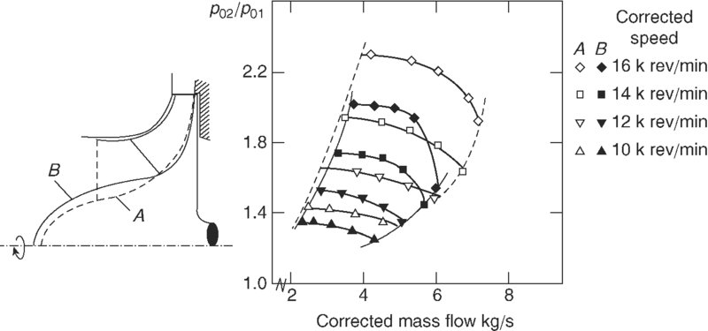
FIGURE 9.17 Performance maps of two impellers (A) with and (B) without inducer. Source: Eckhardt 1977. Courtesy of German Government
9.6 Impeller Exit Flow and Blockage Effects
We have introduced the phenomenon of slip at the impeller exit. The turning of the relative flow in the opposite direction to that of the rotor starts inside the impeller passage. We have graphically depicted the relative streamlines in the impeller in Figure 9.3d. The accumulation of the flow on the pressure side results in a jet-like behavior and the sparse low-momentum flow on the suction side of the impeller vanes gives an appearance of the wake (or deficit momentum) flow. This behavior at the exit of the centrifugal compressor impellers is known as the jet-wake flow, first described by Dean and Senoo (1960). Figure 9.18 shows the jet-wake exit flow behavior in a radial impeller. The first observation is that the impeller exit flow is highly nonuniform. Therefore, the one-dimensional approximations that we often make need to be modified to reflect the nonuniform flow behavior. The second implication is that the boundary layer on the suction surface near the impeller exit is likely separated, as schematically shown in Figure 9.18. The combined effects of jet-wake velocity profile and separated flow gives rise to a high level of blockage at the exit.

FIGURE 9.18 The exit flow pattern from an impeller shows a “jetwake” profile
Through the concept of blockage, we define an effective flow area A2eff. The definition of blockage from diffuser studies in Chapter 6is repeated here, where effective and geometrical areas are applied to the impeller exit:
where A2 is the geometric flow area that may be written as
In Equation 9.40, N is the number of the impeller vanes, t is thickness of the blades at the exit, b is the axial span of vanes at 2, and β’2 is the blade sweep angle at the exit (measured from the radial direction). The cosine term in Equation 9.40 gives a projection of the exit area that is in the radial direction. The conclusions from this section are
- One-dimensional flow analysis is totally inadequate and gives erroneous results
- Jet-wake profile and flow separation have to be accounted for by a suitable averaging technique and an estimate of blockage B2, respectively. In either case, more experimental data are needed.
9.7 Efficiency and Performance
Centrifugal compressor efficiency has always lagged its counterpart, the axial-flow compressor, for the same pressure ratio. The flow path is rather torturous as it twists from one plane to another in a centrifugal compressor, thus massive secondary flow and separation losses become imminent. In addition, for high-pressure ratio centrifugal compressors, the flow in the diffuser becomes supersonic and its efficient diffusion rather complex. In a historical perspective presented by Kenny (1984), different loss sources, future design trends, and limitations of centrifugal compressors are discussed. Although it is very difficult, if not impossible, to separate losses in turbomachinery into their components without overlapping, which is double/triple accounting, it is still instructive to expose general loss sources in turbomachinery. In a centrifugal compressor, the losses are attributed to
- Tip clearance loss in an unshrouded impeller
- Secondary flow losses due to flow turning
- Disk friction losses
- Losses due to compressibility effects in the inducer due to shocks and flow separation
- Jet-wake mixing flow losses in the diffuser
- Diffuser compressibility losses due to high absolute Mach numbers
- Flow unsteadiness and vortex shedding in the impeller wake.
Also a comparison of two centrifugal compressors designed for an 8:1 total-to-static pressure ratio and their efficiencies at off-designare shown in Figure 9.19 (also from Kenny). Note that the efficiencies are listed for total exit-to-static inlet state of the gas, as well as the pressure ratio. For a Mach 0.5 (absolute inlet) flow, the ratio of total-to-static pressure is [1 + (0.2)(0.5)2]3.5 ≅ 1.186, therefore an 8:1 design total-static pressure ratio means a totalto-total pressure ratio of πs ≅ 6.74. Although centrifugal compressors are less efficient; they can produce stage pressure ratios outside the reach of the axial-flow compressors. The centrifugal compressors represent the compressor of choice for small aircraft engines, auxiliary power units, industrial applications, as well as automotive turbochargers.
Figure 9.20 shows a T–s diagram that is used in defining total-to-static efficiency of centrifugal compressors. Advances in centrifugal compressor design are demonstrated by an increase in total-to-static pressure ratio and adiabatic efficiency as shown in Figures 9.21 and 9.22 (from Kenny, 1984).
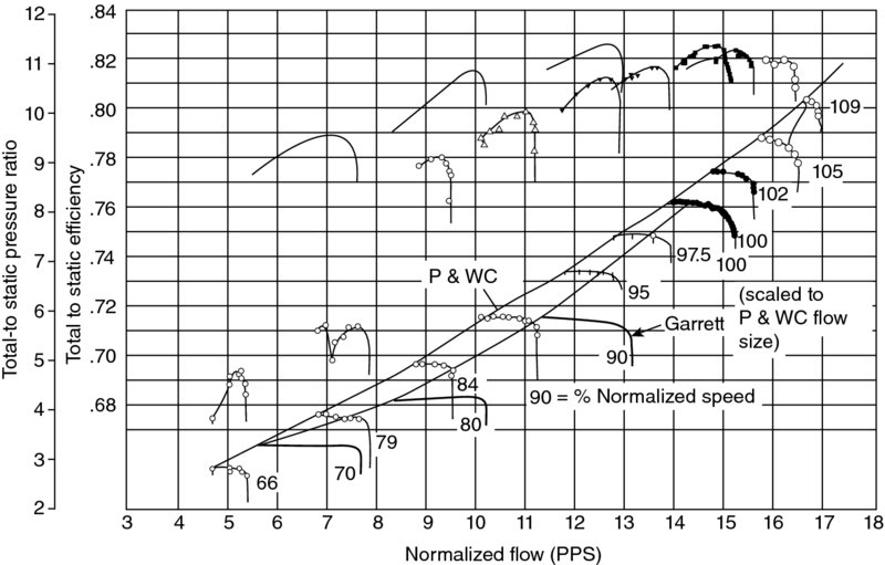
FIGURE 9.19 The performance map for two centrifugal compressors with an 8:1 total-static design pressure ratio. Source: Kenny 1984. Reproduced with permission from SAE International

FIGURE 9.20 T–s diagram used in defining the total-to-static efficiency of a centrifugal compressor

FIGURE 9.21 Advances in centrifugal compressor performance. Source: Kenny 1984. Reproduced with permission from SAE International

FIGURE 9.22 Historic perspective on centrifugal compressor (total to static) pressure ratio. Source: Kenny 1984. Reproduced with permission from SAE International
9.8 Summary
Centrifugal compressors achieve high compression per stage that is predominantly produced by centrifugal force with a large exit-to-inlet impeller radius ratio. The flow area through the inlet is thus a small fraction of the frontal area of the machine. Therefore, the mass flow rate per frontal area is lower in centrifugal than the axial-flow compressors.
The pressure ratio per stage is high, however, with lower adiabatic efficiency than the axial counterpart. The flow path from the inlet to the exit twists and turns, thus secondary flow losses are significant. The phenomenon of slip creates a jet-wake nonuniform velocity profile at the impeller exit. The geometry of the impeller blade passages is characterized by a large wetted perimeter and a small flow area, which makes for an equivalently small hydraulic diameter with large frictional losses. The radial flow from the impeller is decelerated in radial and vaned diffusers. The diffuser exit flow is turned 90° for a follow up combustor or even 180° degrees for the next centrifugal compressor stage. Therefore, staging centrifugal compressors involve turnaround ducts, which make them more cumbersome than axial compressors.
The robust construction of the centrifugal compressors and their high pressure ratio per stage capability make them ideal for small gas turbine engines, auxiliary power units, automotive turbo-chargers, and other industrial uses. The inducer-less and shrouded impellers are used in industrial applications, whereas the unshrouded impellers with inducers that offer lower weight and higher mass flow capability are suitable for aerospace applications.
Classical literature on turbomachinery is found in Stodola’s text (1924, 1927) as well as Traupel’s book (1977). Taylor (1964), Marble (1964), Kerrebrock (1992), Cumpsty (2004) and Dixon (1975) have treated compressors in detail and are recommended for further reading. Historical perspectives presented by Garvin (1998) and St. Peter (1999) compliment the subject. Hill and Peterson’s book (1992) as well as Paduano, Greitzer and Epstein’s review paper (2001) on compression system stability are recommended to the reader.
References
- Busemann, A., “Das Foerderhuehenverhaeltnis radialer Kreiselpumpen mit Logarithmisch-spiraligen Schaufeln, ” Zeitschrift angewandete Mathematik und Mechanik, Vol. 8, No. 5, 1928.
- Cumpsty, N.A., Compressor Aerodynamics, Krieger Publishing Co., Malabar, FL, 2004.
- Dean, R.C. and Senoo, Y., “Rotating Wakes in Vaneless Diffusers, : Transactions of ASME, ” Journal of Basic Engineering, Vol. 82, 1960, pp. 563–574.
- Dixon, S.L., Fluid Mechanics, Thermodynamics of Turbomachinery, 2nd edition, Pergamon Press, Oxford, UK, 1975.
- Eckhardt, D., Vergleichende Stroemungsuntersuchungen an drei Radiaverdichter-Laufraden mit konventionellen Messferfahren, Forschungsbericht Verbrennungskraftmaschinen, Vorhaben 182, Vol. 237, 1977.
- Garvin, R.V., Starting Something Big: The Commercial Emergence of GE Aircraft Engines, AIAA, Inc., Reston, VA, 1998.
- Hill, P.G. and Peterson, C.R., Mechanics and Thermodynamics of Propulsion, 2nd edition, Addison-Wesely, Reading, MA, 1992.
- Kenny, D.P., “The History and Future of the Centrifugal Compressor in Aviation Gas Turbines, ” SAE Paper No. 841635, 1984.
- Kerrebrock, J.L., Aircraft Engines and Gas Turbines, 2nd edition, MIT Press, Cambridge, MA, 1992.
- Marble, F.E., “Three-Dimensional Flow in Turbomachines, ” in Aerodynamics of Turbines and Compressors, Vol. X, Ed. Hawthorne, W.R., Princeton Series on High Speed Aerodynamics and Jet Propulsion, Princeton University Press, Princeton, NJ, 1964.
- Paduano, J.D., Greitzer, E.M., and Epstein, A.H., “Compression System Stability and Active Control, ” Annual Review of Fluid Mechanics, Vol. 33, 2001, pp. 491–517.
- Stanitz, J.D. and Ellis, G.O., “Two-Dimensional Compressible Flow in Centrifugal Compressors with Straight Blades, ” NACA Technical Note 1932, 1949.
- St. Peter, J., The History of Aircraft gas Turbine Engine Development in the United States, International Gas Turbine Institute, Atlanta, GA, 1999.
- Stodola, A., Dampf- und Gasturbinen, Springer Verlag, 1924.
- Stodola, A., Steam and Gas Turbines, Vos. 1 and 2, McGraw-Hill, New York, 1927.
- Taylor, E.S., “The Centrifugal Compressor”, in Aerodynamics of Turbines and Compressors, Ed. Hawthorne, W.R., Princeton Series in High-Speed Aerodynamics and Jet Propulsion, Vol. X, Princeton University Press, Princeton, NJ, 1964.
- Traupel, W., Thermische Turbomaschinen, 3rd edition, Springer Verlag, 1977.
Problems
- 9.1 A centrifugal compressor has 22 radial impellers with an (impeller) exit radius of r2 = 0.25 m. Assuming the mass flow rate through the compressor is
 kg/s, the shaft speed is ω = 10, 000 rpm, and the inlet flow is swirl free, calculate
- the shaft power, ℘s, in kW
- the total temperature rise in the compressor (assume γ = 1.4 and cp = 1004 J/kg · K)
- 9.2 Size the exit radius of a centrifugal compressor impeller, r2, that is to reach a tangential Mach number of MT = 1.5. The shaft rotational speed is 25, 000 rpm and the inlet flow condition is characterized by
- 9.3 We are interested in a parametric study of the diffusion factor for an inducer section of an impeller. We know from Equation 9.39b that

There are three nondimensional groups that appear in the above equation.
- impeller radius ratio r1/r2
- ratio of impeller tip Mach umber to the inlet axial Mach number MT2/Mz1
- inducer solidity σi
Graph Dinducer versus one of the three nondimensional groups while keeping the other two groups constant.
- 9.4 A centrifugal compressor has no inlet guide vanes and thus zero preswirl. The axial Mach number is M1 = 0.5 and is uniform at the impeller face. The inlet condition is entirely known, p1 = 100 kPa, T1 = 288 K, and the geometry of the inlet, r1h = 10 cm and r1t = 25 cm. The exit radius is r2 = 0. 35 cm and shaft rotational speed is 10, 000 rpm. The centrifugal compressor has 20 radial impeller blades.
Assuming the compressor polytropic efficiency ec = 0.85, calculate
- mass flow rate
 (in kg/s)
 - absolute swirl velocity at the impeller exit, Cθ2, in m/s
- compressor specific work, at the pitchline, wc, in kJ/kg
- compressor shaft power in kW
- compressor pressure ratio πs
- exit (absolute) Mach number at 2, M2, assuming Cr2 = Cz1
- swirl velocity at the exit of the radial vaneless diffuser
(assuming zero frictional losses in the diffuser) and radius of 45 cm
- mass flow rate
- 9.5 A centrifugal compressor has 25 impeller blades of radial design. The rotor exit diameter is r2 = 0.4 m, and its rotational speed is ω = 8000 rpm. Assuming the inlet to rotor flow is purely axial and the air mass flow rate is
 = 25 kg/s through the compressor, calculate
- compressor shaft power, ℘c in, MW
- (time rate of change of) angular momentum at the rotor exit

- 9.6 The inlet flow to a radial (vaneless) diffuser has a swirl component of Cθ2 = 200 m/s and a radial component of Cr2 = 100 m/s. The impeller exit radius r2 = 25 cm and the flow static pressure and temperature are

Assuming inviscid flow in the radial diffuser, with γ = 1.4 and R = 287 J/Kg · K, calculate
- Cr(r)
- Cθ(r)
- 9.7 A centrifugal compressor discharge pressure and temperature are measured to be

The inlet flow is purely axial with Cz1 = 100 m/s and the inlet total pressure and temperature are
Calculate
- total-to-static pressure ratio pt3/p1
- total-to-total pressure ratio
- total-to-static adiabatic efficiency ηTS
- total-to-total adiabatic efficiency ηTT
- polytropic efficiency ec for total-static and total-total processes
- 9.8 To eliminate the inducer from a centrifugal compressor impeller, we need to induce a swirl profile in the incoming flow (known as preswirl) that is in the direction of the rotor and its relative flow to the impeller is purely axial. This task is done through an IGV.
For an inducer-less impeller of

Calculate
- swirl profile Cθ1 (r)
- absolute flow angle α1 (r)
- the IGV twist from hub-to-tip, assuming a constant deviation angle with span
- 9.9 The inlet static pressure to an impeller is p1 = 100 kPa and its exit static pressure is p2 = 200 kPa with inlet relative dynamic pressure q1r = 140 kPa. Treating the impeller as a diffuser, assuming γ = 1.4, calculate
- inlet relative Mach number M1r
- static pressure recovery coefficient CPR
- 9.10 A radial diffuser has an exit-to-inlet radius ratio r3/r2 of 4. Assume the flow is incompressible and the fluid is inviscid. Calculate
- the diffuser area ratio A3/A2
- exit-to-inlet radial velocity ratio Cr3/Cr2
- exit-to-inlet swirl ratio Cθ3/Cθ2
- static pressure rise coefficient or static pressure recovery CPR
- 9.11 A centrifugal compressor has a total pressure ratio of pt3/pt1 = 8. Calculate and graph this compressor’s total-to-static pressure ratio pt3/p1 for a range of inlet Mach numbers M1 from 0.25 to 0.75 in steps of 0.05. Assume γ = 1.4.
- 9.12 The total-to-total compressor adiabatic efficiency for a centrifugal compressor is ηTT = 0.78. The compressor total pressure ratio is pt3/pt1 = 7. Assuming the inlet Mach number is M1 = 0. 4 and γ = 1.4, calculate
- total-to-static pressure ratio
- total temperature ratio Tt3/Tt1
- total-to-static adiabatic efficiency ηTS.
- 9.13 A backswept impeller has a tip speed of U2 = 366 m/s and the impeller blade exit angle is β′2 = 30°. The radial velocity at the impeller exit is Cr2 = 125 m/s. Stagnation speed of sound at the impeller inlet is at1 = 340 m/s, assuming the inlet flow is purely axial, and the slip angle at the impeller exit is 6°, i.e., β2 − β′2 = 6°, calculate
- slip factor
- Mach index ΠM
- Impeller specific work, wc, in kJ/kg
- stage total temperature ratio τstage
- stage total pressure ratio if ec = 0.89
Assume γ = 1.4 and cp = 1004 J/Kg · K.

- slip factor
- 9.14 A forward-swept impeller has a tip speed of U2 = 400 m/s and the impeller blade exit angle is β′2 = −30°. The radial velocity at the impeller exit is Cr2 = 100 m/s. Stagnation speed of sound at the impeller inlet is at1 = 330 m/s, assuming the inlet flow is purely axial and the slip angle at the impeller exit is −6°, i.e., β′2 − β2 = −6°, calculate
- slip factor
- Mach index ΠM
- impeller specific work, wc, in kJ/kg
- stage total temperature ratio τstage
- stage total pressure ratio if ec = 0.89.
- slip factor
- 9.15 A 19-bladed radial impeller has an exit radius r2 = 25 cm. The impeller width at the exit is b = 1 cm. We wish to calculate and compare some impeller exit flow areas with successive levels of detail.
Case 1
Assume the individual trailing edge thickness of impeller blades is zero, i.e., t = 0, and calculate the geometric flow area.
Case 2
Assume the individual trailing edge thickness is t = 2 mm (per blade), and calculate the geometric flow area at the impeller exit.
Case 3
Assume the impeller exit blockage is 10% and now calculate the effective flow area.
Assuming the same slip factor between the three cases, relate the average radial velocity Cr2 in cases 1, 2, and 3.
- 9.16 Air enters a centrifugal compressor at pt1 = 101 kPa, Tt1 = 288 K, and purely in an axial direction with Mz = 0.4. Assuming the impeller radius at the exit is r2 = 25 cm and the impeller is of radial design with slip factor = 0.9 and MT2 = 1.5, calculate
- U2 in m/s
- specific work, wc, in kJ/kg
- impeller exit total temperature, Tt2, in K
- shaft rotational speed, ω, in rpm
- 9.17 The flow pattern at the exit of a radial centrifugal compressor impeller shows a jet-wake behavior, as shown in Figure 9.18, which is reproduced here with additional descriptions. In order to estimate the blockage, we assume that the wake region has zero momentum and is of angular extent θ2, wake (per passage) at the impeller exit, as shown. The number of impeller blades is N, and the blade thickness at the exit is t (note the blade sweep angle is zero).
Calculate
- the geometric flow area at 2 in terms of r2, t, N, and b
- the effective flow area in terms of θ2, wake
- the blockage B2

- 9.18 Consider a radial diffuser in a centrifugal compressor with straight radial impeller, as shown. The radial velocity at the impeller exit is Cr2 = 150 m/s, the tangential velocity Cθ2 = 250 m/s and the slip factor is = 0.90. The stagnation temperature at the inlet to the impeller is Tt1 = 298 K.
Assuming inlet flow to the centrifugal compressor is swirl free, i.e., Cθ1 = 0, calculate
- absolute Mach number, M2
- swirl at the exit of the radial diffuser, Cθ3, assuming inviscid flow
- exit swirl, Cθ3, if the average retarding torque acting on the fluid by the wall is 5% of (time rate of change of the) fluid angular momentum at 2.

- 9.19 A centrifugal compressor impeller has 20 straight blades. The exit radius of the impeller is r2 = 0.30 m and the angular speed is ω = 14, 500 rpm. The inlet flow to the compressor has zero preswirl and the axial velocity is Cz1 = 150 m/s. The impeller exit has the radial velocity component Cr2 that is equal to Cz1.
Assuming the speed of sound at the inlet to compressor is a1 = 300 m/s, calculate
- Mach index, ΠM
- impeller exit absolute swirl, Cθ2, in m/s
- specific work of the rotor, wc, in kJ/kg
- impeller exit absolute Mach number, M2
- compressor total temperature ratio, τc

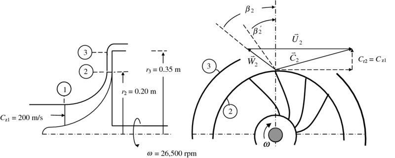
- 9.20 A centrifugal compressor impeller has 30 backswept blades with β′2 = 20°. The inlet flow condition to the compressor is purely axial with Cz1 = 200 m/s and its total pressure and temperature are: pt1 = 100 kPa and Tt1 = 288 K, respectively. The impeller rim is at a radius of r2 = 0.2 m and the shaft rotational speed is ω = 26, 500 rpm. The radial velocity at the impeller exit is equal to the inlet axial velocity, as shown. Assuming the vaneless radial diffuser has an exit radius of r3 = 0.35 m and further assuming that the flow in the radial diffuser is inviscid with gas properties γ = 1.4 and R = 287 J/kgK, calculate
- impeller rim speed, U2, in m/s
- impeller (actual) exit swirl, Cθ2, in m/s
- specific work of the compressor, wc, in kJ/kg
- impeller absolute exit Mach number, M2
- swirl velocity at the diffuser exit, Cθ3, in m/s
- radial velocity at the diffuser exit, Cr3, in m/s (neglecting density variations in the diffuser)
- 9.21 A centrifugal compressor impeller is of radial design and has 18 blades. The impeller exit radius is at r2 = 0.30 m. The wheel rim speed is U2 = 400 m/s. Assuming that flow in compressor inlet is swirl free, the axial velocity at the inlet and the radial velocity at the exit of the impeller are equal, i.e., Cz1 = Cr2 = 150 m/s, with Tt1 = 288 K, pt1 = 100 kPa, γ = 1.4 and cp = 1004 J/kg · K, calculate
- absolute swirl at the impeller exit, Cθ2, in m/s
- absolute Mach number at the impeller exit, M2
- absolute radial and tangential velocities at the radial diffuser exit, Cr3 and Cθ3, in m/s
(Assume the fluid is incompressible and inviscid in the radial diffuser)

- 9.22 A centrifugal compressor has 20 radial impeller blades that rotate at ω = 18, 500 rpm. The impeller exit radius is r2 = 0.20 m. Assuming that the inlet flow is swirl free, calculate
- impeller exit (absolute) swirl, Cθ2, in m/s
- impeller rim tangential Mach number, MT = ωr2/a1
- speed of sound, a2, in m/s at the impeller exit

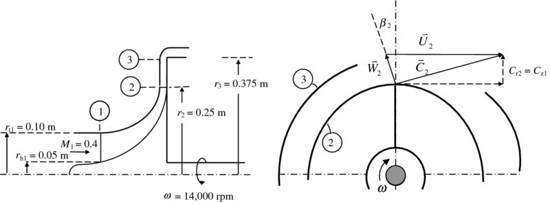
- 9.23 A centrifugal compressor impeller has 20 straight impeller blades. The inlet flow condition to the compressor is purely axial with M1 = 0.4. The geometric parameters of the centrifugal compressor are: rh1 = 0.05 m, rt1 = 0.1 m, r2 = 0.25 m and r3 = 0.375 m. The shaft rotational speed is ω = 14, 000 rpm. The static pressure and temperature at the inlet are p1 = 90 kPa and T1 = 255 K, respectively. The radial velocity at the impeller exit is equal to the inlet axial velocity, i.e., Cr2 = Cz1 and the compressor polytropic efficiency is ec = 0.85. Assuming the radial diffuser is vaneless and the flow in the radial diffuser is inviscid with gas properties γ = 1.4 and R = 287 J/kg · K, calculate
- flow area at the inlet to the centrifugal compressor, A, in m2
- inlet axial velocity, Cz1, in m/s
- inlet density, ρ1, in kg/m3
- the mass flow rate,
 , in kg/s
 - impeller rim speed, U2, in m/s
- impeller (actual) exit swirl, Cθ2, in m/s
- compressor shaft power, ℘c, in kW
- impeller absolute exit Mach number, M2
- swirl velocity at the diffuser exit, Cθ3, in m/s
- stage total pressure ratio, πc
- 9.24 The corrected mass flow rate at the inlet to a centrifugal compressor is
 and the axial Mach number at the compressor face is Mz1 = 0.5. For the hub-to-tip radius ratio of the impeller equal to 0.1, i.e., rh1/rt1 = 0.1, calculate
- inlet area, A1, in m2
- hub and tip radii, rh1 and rt1, in cm
- shaft speed, ω, for the impeller inlet relative tip Mach number to be 0.8, i.e., (M1r)tip
Assume gas total temperature at the impeller inlet is 288 K, γ = 1.4 and R = 287 J/kgK
- 9.25 A centrifugal compressor discharge static pressure is p3 = 352 kPa and its total temperature is Tt3 = 444 K. The flow at the impeller inlet has an axial component with Cz1 = 150 m/s and a preswirl component with Cθ1 = 56 m/s. The inlet total pressure and temperature are the standard sea-level conditions, i.e., pt1 = 101 kPa and Tt1 = 288 K, respectively. Assuming the compressor polytropic efficiency is ec = 0.88, calculate
- compressor total pressure ratio, pt3/pt1
- static pressure ratio, p3/p1, across the compressor
- exit Mach number, M3
- compressor specific work, wc, in kJ/kg
Assume fluid properties are: γ = 1.4 and cp = 1004 J/kgK