CHAPTER 2 Compressible Flow with Friction and Heat: A Review
2.1 Introduction
Schlieren visualization of waves around an X-15 model in a supersonic wind tunnel. Source: Courtesy of NASA
The study of propulsion is intimately linked to the understanding of internal fluid mechanics. This means that duct flows are of prime interest to propulsion. The physical phenomena in a real duct include the following effects:
Friction
Heat transfer through the walls
Chemical reaction within the duct
Area variation of the duct
Compressibility effects, e.g. appearance of shocks
The laws of thermodynamics govern the relationship between the state variables of the gas, namely density ρ, pressure p, absolute temperature T, entropy s, internal energy e, and derived properties such as enthalpy h and specific heats at constant pressure and volume, cp and cv, respectively. In addition to the laws of thermodynamics, the fluid flow problems need to obey other conservation principles that were introduced in Newtonian mechanics. These are conservation of mass and momentum as described in classical mechanics. Since the study of gas turbine engines and propulsion in undergraduate curricula in mechanical and aerospace engineering follows the introductory courses in thermo-fluid dynamics, we shall review only the principles that have a direct impact on our study of jet engines.
The purpose of this chapter is thus to provide a review of the working principles in aerothermodynamics, which serve as the foundation of propulsion. The reader should consult textbooks on thermodynamics, such as the classical work of Sonntag, Borgnakke, and Van Wylen (2003), and modern fluid mechanics books, such as Munson, Young, and Okiishi (2006) or John Anderson’s books on aerodynamics (2005). For detailed exposition of compressible flow, the two volumes written by Shapiro (1953) should be consulted.
2.2 A Brief Review of Thermodynamics
To get started, we need to characterize the medium that flows through the duct. In gas turbine engines the medium is a perfect gas, often air. The perfect gas law that relates the pressure, density, and the absolute temperature of the gas may be derived rigorously from the kinetic theory of gases. Prominent assumptions in its formulation are (1) intermolecular forces between the molecules are negligibly small and (2) the volume of molecules that occupy a space is negligibly small and may be ignored. These two assumptions lead us to
In general, the specific heats at constant pressure and volume are functions of gas temperature,
(2.5)
(2.6)
The gas is then called a thermally perfect gas. There is often a simplifying assumption of constant specific heats, which is a valid approximation to gas behavior in a narrow temperature range. In this case,
(2.5a)
(2.6a)
The gas is referred to as a calorically perfect gas.
The first law of thermodynamics is the statement of conservation of energy for a system of fixed mass m, namely,
where the element of heat transferred to the system from the surrounding is considered positive and on a per-unit-mass basis is δq with a unit of energy/mass, e.g., J/kg. The element of work done by the gas on the surrounding is considered positive and per-unit-mass of the gas is depicted by δw. The difference in the convention for positive heat and work interaction with the system explains the opposite sides of equation where the two energy exchange terms are located in Equation 2.7, otherwise they both represent energy exchange with the system. The net energy interaction with the system results in a change of energy of the system; where again on a per-unit-mass basis is referred to as de. The three terms of the first law of thermodynamics have dimensions of energy per mass. The elemental heat and work exchange are shown by a delta “δ” symbol instead of an exact differential “d” as in “de.” This is in recognition of path-dependent nature of heat and work exchange, which differ from the thermodynamic property of the gas “e, ” which is independent of the path, i.e.,
(2.8)
rather
(2.9)
Whereas in the case of internal energy (or any other thermodynamic property),
(2.10)
Note that in the eyes of the first law of thermodynamics, there is no distinction between heat and mechanical work exchange with the system. It is their “net” interaction with the system that needs to be accounted for in the energy balance. The application of the first law to a closed cycle is of importance to engineering and represents a balance between the heat and work exchange in a cyclic process, i.e.,
(2.11)
Also, for an adiabatic process, i.e., δq = 0, with no mechanical exchange of work, i.e., δw = 0, the energy of a system remains constant, namely e1 = e2 = constant. We are going to use this principle in conjunction with a control volume approach in the study of inlet and exhaust systems of an aircraft engine.
The second law of thermodynamics introduces the absolute temperature scale and a new thermodynamic variable s, the entropy. It is a statement of impossibility of a heat engine exchanging heat with a single reservoir and producing mechanical work continuously. It calls for a second reservoir at a lower temperature where heat is rejected to by the heat engine. In this sense, the second law of thermodynamics distinguishes between heat and work. It asserts that all mechanical work may be converted into system energy whereas not all heat transfer to a system may be converted into system energy continuously. A corollary to the second law incorporates the new thermodynamic variable s and the absolute temperature T into an inequality, known as the Clausius inequality,
(2.12)
where the equal sign holds for a reversible process. The concept of irreversibility ties in closely with frictional losses, viscous dissipation, and the appearance of shock waves in supersonic flow. The pressure forces within the fluid perform reversible work, and the viscous stresses account for dissipated energy of the system (into heat). Hence the reversible work done by a system per unit mass is
(2.13)
where v is the specific volume, which is the inverse of fluid density ρ. A combined first and second law of thermodynamics is known as the Gibbs equation, which relates entropy to other thermodynamic properties, namely
(2.14)
Although it looks as if we have substituted the reversible forms of heat and work into the first law to obtain the Gibbs equation, it is applicable to irreversible processes as well. Note that in an irreversible process, all the frictional forces that contribute to lost work are dissipated into heat. Now, we introduce a derived thermodynamic property known as enthalpy, h, as
This derived property, that is, h, combines two forms of fluid energy, namely internal energy (or thermal energy) and what is known as the flow work, pv, or the pressure energy. The other forms of energy such as kinetic energy and potential energy are still unaccounted by the enthalpy h. We shall account for the other forms of energy by a new variable called the total enthalpy later in this chapter.
Now, let us differentiate Equation 2.15 and substitute it in the Gibbs equation, to get
By expressing enthalpy in terms of specific heat at constant pressure, via Equation 2.3, and dividing both sides of Equation 2.16 by temperature T, we get
An assumption of a calorically perfect gas will enable us to integrate the first term on the right-hand side of Equation 2.18, i.e.,
(2.19)
Otherwise, we need to refer to a tabulated thermodynamic function defined as
(2.20)
From the definition of enthalpy, let us replace the flow work, pv, term by its equivalent from the perfect gas law, i.e., RT, and then differentiate the equation as
(2.21)
Dividing through by the temperature differential dT, we get
(2.22a)
(2.22b)
This provides valuable relations among the gas constant and the specific heats at constant pressure and volume. The ratio of specific heats is given by a special symbol γ due to its frequency of appearance in compressible flow analysis, i.e.,
(2.23)
In terms of the ratio of specific heats γ and R, we express cp and cv as
The ratio of specific heats is related to the degrees of freedom of the gas molecules, n, via
(2.25)
The degrees of freedom of a molecule are represented by the sum of the energy states that a molecule possesses. For example, atoms or molecules possess kinetic energy in three spatial directions. If they rotate as well, they have kinetic energy associated with their rotation. In a molecule, the atoms may vibrate with respect to each other, which then creates kinetic energy of vibration as well as the potential energy of intermolecular forces. Finally, the electrons in an atom or molecule are described by their own energy levels (both kinetic energy and potential) that depend on their position around the nucleus. As the temperature of the gas increases, the successively higher energy states are excited; thus the degrees of freedom increases. A monatomic gas, which may be modeled as a sphere, has at least three degrees of freedom, which represent translational motion in three spatial directions. Hence, for a monatomic gas, under “normal” temperatures the ratio of specific heats is
(2.26)
A monatomic gas has negligible rotational energy about the axes that pass through the atom due to its negligible moment of inertia. A monatomic gas will not experience a vibrational energy, as vibrational mode requires at least two atoms. At higher temperatures, the electronic energy state of the gas is affected, which eventually leads to ionization of the gas. For a diatomic gas, which may be modeled as a dumbbell, there are five degrees of freedom under “normal” temperature conditions, three of which are in translational motion and two of which are in rotational motion. The third rotational motion along the intermolecular axis of the dumbbell is negligibly small. Hence for a diatomic gas such as air (near room temperature), hydrogen, nitrogen, and so on, the ratio of specific heats is
(2.27a)
At high temperatures, molecular vibrational modes and the excitation of electrons add to the degrees of freedom and that lowers γ. For example, at ∼ 600 K vibrational modes in air are excited, thus the degrees of freedom of diatomic gasses are initially increased by 1, that is, it becomes 5 + 1 = 6, when the vibrational mode is excited. Therefore, the ratio of specific heats for diatomic gases at elevated temperatures becomes
(2.27b)
The vibrational mode represents two energy states corresponding to the kinetic energy of vibration and the potential energy associated with the intermolecular forces. When fully excited, the vibrational mode in a diatomic gas, such as air, adds 2 to the degrees of freedom, that is, it becomes 7. Therefore, the ratio of specific heats becomes
(2.27c)
For example, air at 2000 K has its translational, rotational, and vibrational energy states fully excited. This temperature level describes the combustor or afterburner environment. Gases with a more complex structure than a diatomic gas have mote degrees of freedom, and thus their ratio of specific heats is less than 1.4. Figure 2.1 (from Anderson, 2003) shows the behavior of a diatomic gas from 0 to 2000 K. The nearly constant specific heat ratio between 3 and 600 K represents the calorically perfect gas behavior of a diatomic gas such as air with γ = 1.4. Note that near absolute zero (0 K), cv/R → 3/2; therefore, a diatomic gas ceases to rotate and thus behaves like a monatomic gas, that is, it exhibits the same degrees of freedom as a monatomic gas, that is, n = 3, γ = 5/3.
FIGURE 2.1Temperature dependence of specific heat for a diatomic gas. Source: Anderson 2003, Fig. 16.11, p. 613. Reproduced with permission from McGraw Hill
2.3 Isentropic Process and Isentropic Flow
For an isentropic process, where entropy remains constant, the Gibbs equation relates the pressure and temperature ratios by an isentropic exponent:
Now, using the perfect gas law by replacing the temperature ratio by pressure and density ratios in Equation 2.28 and simplifying the exponents, we get
2.4 Conservation Principles for Systems and Control Volumes
A system is a collection of matter of fixed identity, hence fixed mass, whereas a control volume is a fixed region in space with fluid crossing its boundaries. A control volume approach seems to be a more practical method of treating the fluid flow problems in gas turbine engines. However, all the classical laws of Newtonian physics are written for a matter of fixed mass, i.e., the system approach. For example, the mass of an object (in our case a collection of matter described by a system) does not change with time, is a Newtonian mechanics principle. The counterpart of that expressed for a control volume is known as the continuity equation and is derived as follows. The starting point is the system expression, namely
(2.30)
We now express mass as the integral of density over volume
(2.31)
where V(t) is the volume of the system at any time t. Note that to encompass the entire original mass of the gas in the system, the boundaries of the system become a function of time. Expression 2.31 is a derivative with respect to time of an integral with time-dependent limits. The Leibnitz rule of differentiating such integrals is the bridge between the system and the control volume approach, namely
The limits of the integrals on the right-hand side (RHS) of Equation 2.32 describe a volume V(t0) and a closed surface S(t0), which represents the boundaries of the system at time t0. We choose our control volume to coincide with the boundaries of the system at time t0 Since the time t0 is arbitrary, the above equation represents the control volume formulation for the medium, namely our continuity equation or law of conservation of mass for a control volume is written as
The fluid velocity vector is and represents a unit vector normal to the control surface and pointing outward. The first integral in Equation 2.33 accounts for unsteady accumulation (or depletion) of mass within the control volume and, of course, vanishes for steady flows. We may demonstrate this by switching the order of integration and differentiation for the first integral, that is,
(2.34)
A positive value depicts mass accumulation in the control volume and a negative value shows mass depletion. The second integral takes the scalar product of the fluid velocity vector and the unit normal to the control surface. Therefore, it represents the net crossing of the mass through the control surface per unit time. Flow enters a control volume through one or more inlets and exits the control volume through one or more exits. There is no mass crossing the boundaries of a control volume at any other sections besides the “inlets” and “outlets.” Since the dot product of the velocity vector and the unit normal vector vanishes on all surfaces of the control volume where mass does not cross the boundaries, the second integral makes a contribution to the continuity equation through its inlets and outlets, namely
We also note that a unit normal at an inlet points in the opposite direction to the incoming velocity vector, therefore the mass flux at an inlet contributes a negative value to the mass balance across the control volume (through a negative dot product). An outlet has a unit normal pointing in the same direction as the velocity vector, hence contributes positively to the mass balance in the continuity equation. In general, the inlet and exit faces of a control surface are not normal to the flow, but still the angle between the normal and the velocity vector is obtuse for inlets and acute for exits, hence a negative and a positive dot product over the inlets and outlets, respectively. Therefore, the net flux of mass crossing the boundaries of a control volume, in a steady flow, is zero. We may assume a uniform flow over the inlet and exits of the control volume, to simplify the integrals of Equation 2.35, to
(2.36)
The product VA in the above equation is more accurately written as VnA or VAn where a normal component of velocity through an area A contributes to the mass flow through the area, or equivalently, the product of velocity and a normal projection of the area to the flow contributes to the mass flow through the boundary. Often the subscript “n” is omitted in the continuity equation for convenience; however, it is always implied in writing the mass flow through a boundary. To write the conservation of mass for a control volume, let us combine the unsteady term and the net flux terms as
(2.37)
where the mass flow rate is now given the symbol (with units of kg/s, lbm/s, or slugs/s). We note that the difference between a positive outgoing mass and a negative incoming mass appears as a mass accumulation or depletion in the control volume. If the exit mass flow rate is higher than the inlet mass flow rate, then mass depletes within the control volume and vice versa.
The momentum equation, according the Newtonian mechanics, relates the time rate of change of linear momentum of an object of fixed mass to the net external forces that act on the object. We may write this law as
(2.38)
Again, we propose to write the mass as the volume integral of the density within the system as
(2.39)
Equation 2.39 is suitable for a system. We apply Leibnitz’s rule to the momentum equation to arrive at the control volume formulation, namely
(2.40)
The first integral measures the unsteady momentum within the control volume and vanishes identically for a steady flow. The second integral is the net flux of momentum in and out of the control surface. Assuming uniform flow at the boundaries of the control surface inlets and outlets, we may simplify the momentum equation to a very useful engineering form, namely
Note that momentum equation (2.40a) is a vector equation and a shorthand notation for the momentum balance in three spatial directions. For example, in Cartesian coordinates, we have
In cylindrical coordinates (r, θ, z), we may write the momentum equation as
(2.42a)
(2.42b)
(2.42c)
We may write these equations in spherical coordinates (r, θ, ) as well. The force terms in the momentum equation represent the net external forces exerted on the fluid at its boundaries and any volume forces, known as body forces, such as gravitational force. If the control volume contains/envelopes an object, then the force acting on the fluid is equal and opposite to the force experienced by the body. For example a body that experiences a drag force D imparts on the fluid a force equal to −D.
The law of conservation of energy for a control volume starts with the first law of thermodynamics applied to a system. Let us divide the differential form of the first law by an element of time dt to get the rate of energy transfer, namely
where the equation is written for the entire mass of the system. The energy E is now represented by the internal energy e times mass, as well as the kinetic energy of the gas in the system and the potential energy of the system. The contribution of changing potential energy in gas turbine engines or most other aerodynamic applications is negligibly small and often ignored. We write the energy as the mass integral of specific energy over the volume of the system, and apply Leibnitz’s rule of integration to get the control volume version, namely
The first term on the RHS of Equation 2.44 is the time rate of change of energy within the control volume, which identically vanishes for a steady flow. The second integral represents the net flux of fluid power (i.e., the rate of energy) crossing the boundaries of the control surface. The rates of heat transfer to the control volume and the rate of mechanical energy transfer by the gases inside the control volume on the surrounding are represented by and terms in the energy equation (2.43). Now, let us examine the forces at the boundary that contribute to the rate of energy transfer. These surface forces are due to pressure and shear acting on the boundary. The pressure forces act normal to the boundary and point inward, that is, opposite to ,
(2.45)
To calculate the rate of work done by a force, we take the scalar product of the force and the velocity vector, namely
Now, we need to sum this elemental rate of energy transfer by pressure forces over the surface, via a surface integral, that is,
(2.47)
Since the convention on the rate of work done in the first law is positive when it is performed “on” the surroundings, and Equation 2.46 represents the rate of work done by the surroundings on the control volume, we need to incorporate an additional negative factor for this term in the energy equation. The rate of energy transfer by the shear forces is divided into a shaft power ℘s that crosses the control surface in the form of shaft shear and the viscous shear stresses on the boundary of the control volume. Hence,
(2.48)
Let us combine the expression 2.48 with Equations 2.44 and 2.43 to arrive at a useful form of the energy equation for a control volume, that is,
(2.49)
The closed surface integrals on the left-hand side (LHS) may be combined and simplified to
We may replace the internal energy and the flow work terms in Equation 2.50 by enthalpy h and define the sum of the enthalpy and the kinetic energy as the total or stagnation enthalpy, to get
(2.51)
where the total enthalpy ht is defined as
(2.52)
In steady flows the volume integral that involves a time derivative vanishes. The second integral represents the net flux of fluid power across the control volume. The terms on the RHS are the external energy interaction terms, which serve as the drivers of the energy flow through the control volume. In adiabatic flows, the rate of heat transfer through the walls of the control volume vanishes. In the absence of shaft work, as in inlets and nozzles of a jet engine, the second term on the RHS vanishes. The rate of energy transfer via the viscous shear stresses is zero on solid boundaries (since velocity on solid walls obeys the no slip boundary condition) and nonzero at the inlet and exit planes. The contribution of this term over the inlet and exit planes is, however, small compared with the net energy flow in the fluid, hence neglected.
The integrated form of the energy equation for a control volume, assuming uniform flow over the inlets and outlets, yields a practical solution for quick engineering calculations
The summations in Equation 2.53 account for multiple inlets and outlets of a general control volume. In flows that are adiabatic and involve no shaft work, the energy equation simplifies to
(2.54)
For a single inlet and a single outlet, the energy equation is even further simplified, as the mass flow rate also cancels out, to yield
(2.55)
Total or stagnation enthalpy then remains constant for adiabatic flows with no shaft power, such as inlets and nozzles or across shock waves.
2.5 Speed of Sound & Mach Number
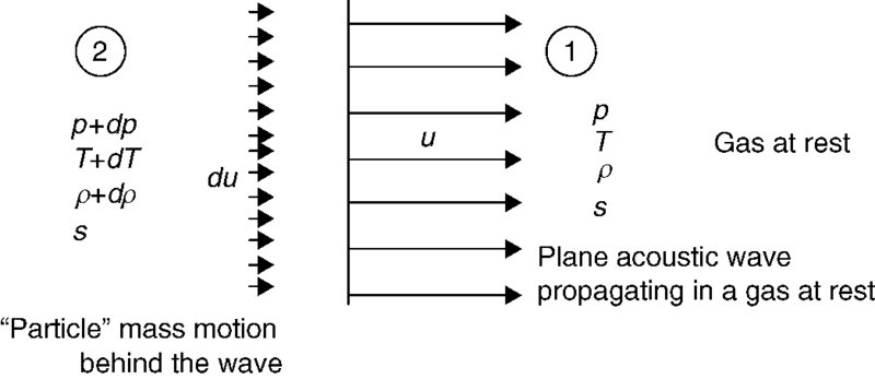
Sound waves are infinitesimal pressure waves propagating in a medium. The propagation of sound waves, or acoustic waves, is reversible and adiabatic, hence isentropic. Since sound propagates through collision of fluid molecules, the speed of sound is higher in liquids than gas. The derivation of the speed of sound is very simple and instructive. Assume a plane sound wave propagates in a medium at rest with speed u. The fluid behind the wave is infinitesimally set in motion at the speed du with an infinitesimal change of pressure, temperature, and density. The fluid ahead of the wave is at rest and yet unaffected by the approaching wave. A schematic drawing of this wave and fluid properties are shown in Figure 2.2.
FIGURE 2.2Propagation of a plane acoustic wave in a gas at rest (an unsteady but isentropic problem)
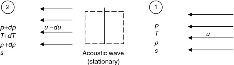
By switching observers from the gas at rest to an observer that moves with the wave at the wave speed u, we change the unsteady wave propagation problem into a steady one. This is known as the Lorentz transformation. The transformed problem is shown in Figure 2.3.
FIGURE 2.3Flow as seen by an observer fixed at the wave (a steady problem)
The fluid static properties, pressure, density, and temperature are independent of the motion of an observer; hence they remain unaffected by the observer transformation. We may now apply steady conservation principles to a control volume, as shown in Figure 2.3. The control volume is a box with its sides parallel to the flow, an inlet and an exit area normal to the flow. We may choose the entrance and exit areas of the box to be unity. The continuity demands
The change of momentum from inlet to exit is shown on the LHS of Equation 2.58. The first parenthesis of each momentum term is the mass flow rate, which is multiplied by the respective flow speeds at the exit and inlet. The driving forces on the RHS of Equation 2.58 are the pressure-area terms in the direction and opposite to the fluid motion, acting on areas that were chosen to be unity. The momentum equation simplifies to
Now, let us substitute the continuity equation (2.57) in the momentum equation (2.59), to get an expression for the square of the acoustic wave propagation in terms of pressure and density changes that occur as a result of wave propagation in a medium at rest
We replaced the ratio of pressure to density by RT from the perfect gas law in Equation 2.62. The symbol we use in this book for the speed of sound is “a, ” hence, local speed of sound in a gas is
The speed of sound is a local parameter, which depends on the local absolute temperature of the gas. Its value changes with gas temperature, hence it drops when fluid accelerates (or expands) and increases when gas decelerates (or compresses). The speed of sound in air at standard sea level conditions is ∼ 340 m/s or ∼1100 ft/s. The type of gas also affects the speed of propagation of sound through its molecular weight. We may observe this behavior by the following substitution:
A light gas, like hydrogen (H2) with a molecular weight of 2, causes an acoustic wave to propagate faster than a heavier gas, such as air with (a mean) molecular weight of 29. If we substitute these molecular weights in Equation 2.64, we note that sound propagates in gaseous hydrogen nearly four times faster than air. Since both hydrogen and air are diatomic gases, the ratio of specific heats remains (nearly) the same for both gases at the same temperature.
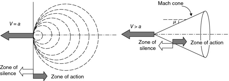
The equation for the speed of propagation of sound that we derived is for a gas at rest. Let us superimpose a uniform collective gas speed in a particular direction to the wave front, then the wave propagates as the vector sum of the two, namely, . For waves propagating normal to a gas flow, we get either (V + a) or (V − a) as the propagation speed of sound. It is the (V − a) behavior that is of interest here. In case the flow is sonic, then (a − a = 0), which will not allow the sound to travel upstream and hence creates a zone of silence upstream of the disturbance. In case the flow speed is even faster than the local speed of sound, that is, known as supersonic flow, the acoustic wave will be confined to a cone. These two behaviors for small disturbances are shown in Figure 2.4.
FIGURE 2.4Acoustic wave propagation in sonic and supersonic flows (or the case of a moving source)
The ratio of local gas speed to the speed of sound is called Mach number, M
(2.65)
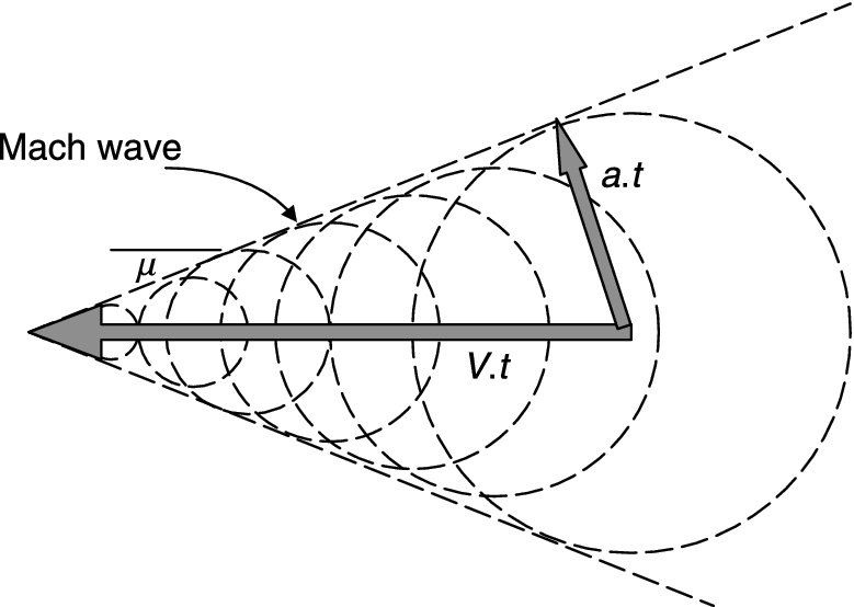
The envelope of the waves that create the zones of action and silence is the Mach wave. It makes a local wave angle with respect to the flow μ, which from the geometry of wave propagation, as shown in Figure 2.5, is
(2.66)
FIGURE 2.5Wave front created by a small disturbance moving at a supersonic speed
2.6 Stagnation State
We define the stagnation state of a gas as the state reached in decelerating a flow to rest reversibly and adiabatically and without any external work. Thus, the stagnation state is reached isentropically. This state is also referred to as the total state of the gas. The symbols for the stagnation state in this book use a subscript “t” for total. The total pressure is pt, the total temperature is Tt, and the total density is ρt. Since the stagnation state is reached isentropically, the static and total entropy of the gas are the same, that is, st = s. Based on the definition of stagnation state, the total energy of the gas does not change in the deceleration process, hence the stagnation enthalpy ht takes on the form
(2.52)
which we defined earlier in this chapter. Assuming a calorically perfect gas, we may simplify the total enthalpy relation 2.52 by dividing through by cp to get an expression for total temperature according to
This equation is very useful in converting the local static temperature and gas speed into the local stagnation temperature. To nondimensionalize Equation 2.67, we divide both sides by the static temperature, that is,
The denominator of the kinetic energy term on the RHS is proportional to the square of the local speed of sound a2 according to Eq 2.63, which simplifies to
Therefore to arrive at the stagnation temperature of the gas, we need to have its static temperature as well as either the gas speed V or the local Mach number of the gas M to substitute in Equations 2.68 or 2.69, respectively. The ratio of stagnation to static temperature of a (calorically perfect) gas is a unique function of local Mach number, according to Equation 2.69. We may also use a spreadsheet tabulation of this function for later use for any gas characterized by its ratio of specific heats γ. From isentropic relations between the pressure and temperature ratio that we derived earlier based on Gibbs equation of thermodynamics, we may now relate the ratio of stagnation to static pressure and the local Mach number via
(2.70)
We used the isentropic relation between the stagnation and static states based on the definition of the stagnation state that is reached isentropically. Also, the stagnation density is higher than the static density according to
(2.71)
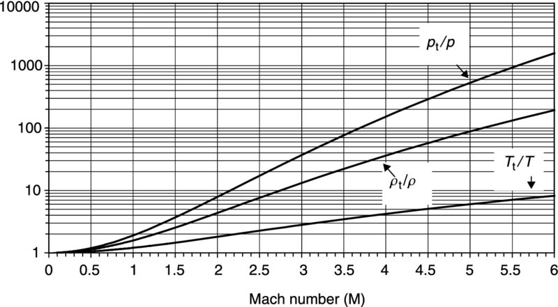
We note that the ratio of stagnation-to-static state of a gas is totally described by the local Mach number and the type of gas γ. The tabulation of these functions, that is, pt/p, Tt/T, and ρt/ρ are made in isentropic tables for a gas described by its ratio of specific heats γ. Figure 2.6 shows the variation of the stagnation state with Mach number for a diatomic gas, such as air (γ = 1.4). The least variation is noted for the stagnation temperature, followed by the density and pressure. To graph these variations (up to Mach 6), we had to use a logarithmic scale, as the total pressure rise with Mach number reaches above one thousand (times the static pressure) while the stagnation temperature stays below ten (times the static temperature). We may examine higher Mach numbers in Figure 2.7. The assumption in arriving at the stagnation state properties relative to the static properties was a calorically perfect gas. The impact of high-speed flight on the atmosphere is to cause molecular dissociation, followed by ionization of the oxygen and nitrogen molecules. A host of other chemical reactions takes place, which result in a violation of our initial assumption. In reality, both the specific heats (cp and cv) are functions of temperature as well as the pressure at hypersonic Mach numbers, that is, M > 5. There are two lessons to be learned here. The first is to always examine the validity of your assumptions; the other is to be cautious about data extrapolations!
FIGURE 2.6Variation of the stagnation state with Mach number for a diatomic gas, γ = 1.4 (For a calorically perfect gas, i.e., cp, cv, and γ are constants)
FIGURE 2.7Variation of stagnation state of gas with flight Mach number for γ = 1.4 (for a calorically perfect gas)
Although the pressure ratio (pt/p) is relieved through real gas effects due to a high-speed flight, it still remains high. Consequently, the high-speed flight has to be scheduled at a high altitude where the static pressure is low. For example, the static pressure at 25 km is only ∼ 2.5% and at 50 km altitude is 0.07% of the sea level pressure.
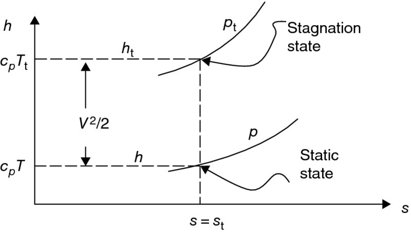
To identify the local static and stagnation states of a gas in a Mollier (h–s) diagram is important in studying propulsion. We use the stagnation enthalpy definition to identify the local stagnation properties of a gas, for example, we start with the static state and then build up a kinetic energy, as in Figure 2.8.
FIGURE 2.8Stagnation and static states of a gas in motion shown on an h–s diagram
We may also apply the Gibbs equation to the stagnation state of the gas to get
(2.72)
For adiabatic flows the first term on the RHS identically vanishes, since the total temperature remains constant. Hence, the total pressure for adiabatic flows with losses, for example, due to frictional losses, always decreases, since the entropy change has to be positive. The exponential relationship between the total pressure ratio and the entropy rise in an adiabatic flow is very useful to propulsion studies and we write it in Equation 2.73
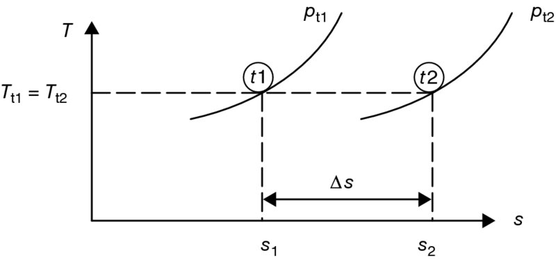
All adiabatic flows with loss result in a drop of total pressure. For example, in a supersonic inlet with shocks and frictional losses in the boundary layer, we encounter a total pressure loss. Since, the total pressure is now cast as a measure of loss via Equation 2.73, it serves as a commodity that propulsion engineers try to preserve as much as possible. The T–s diagram of an adiabatic flow with loss is shown in Figure 2.9.
FIGURE 2.9Adiabatic flow that shows total pressure loss Δpt, e.g., flows containing shocks
2.7 Quasi-One-Dimensional Flow
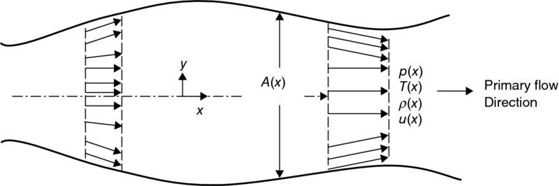
In duct flows with area variations, such as a diffuser or a nozzle, where the boundary layers are completely attached, the streamwise variation of flow variables dominate the lateral variations. In essence, the flow behaves as a uniform flow with pressure gradient in a variable-area duct. A schematic drawing of a duct with area variation is shown in Figure 2.10. The primary flow direction is labeled as “x” and the lateral direction is “y.” Although the flow next to the wall assumes the same slope as the wall, the cross-sectional flow properties are based on uniform parallel flow at the cross-section. The flow area at a cross-section enters the conservation laws, but the variation in the cross-section from the centerline to the wall is neglected. Such flows are called quasi-one-dimensional flows.
FIGURE 2.10Schematic drawing of a variable-area duct with attached boundary layers
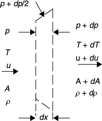
For high Reynolds number flows where the boundary layer is thin compared with lateral dimensions of a duct and assuming an attached boundary layer, the assumption of an inviscid fluid leads to a reasonable approximation of the duct flow. This means that an inviscid fluid model accurately estimates the pressure, temperature, and flow development along the duct axis. Attached boundary layers require a slow variation in the duct area, which is almost invariably the case in propulsion engineering. Inviscid flow analysis also produces a limit performance capability of a component when boundary layers are infinitely thin. In a practical sense, ducts with boundary layer suction approach an inviscid flow model. To develop the quasi-one-dimensional flow equations in a variable-area duct with inviscid fluid, we examine a slice, known as a slab, of the flow and apply the Taylor series approximation to the two sides of the slab. Figure 2.11 shows a thin slice of a duct flow with streamwise length dx separating the two sides of the slab.
FIGURE 2.11Slab of inviscid fluid in a variable-area duct (walls exert pressure on the fluid)
We assume general parameters on one side and step in the x-direction using the Taylor series approximation of an analytical function expanded in the neighborhood of a point. Since the step size dx is small, we may truncate the infinite Taylor series after the first derivative. Note that the walls exert one-half of the incremental pressure (dp/2) over the upstream pressure p, since we take only one-half the step size (dx/2) to reach its center. Now, let us apply the conservation principles to this thin slice of the flow. Continuity demands
(2.74)
Ignoring higher order terms involving the products of two small parameters, such as du · dA, we get
(2.75)
Now dividing both sides by a nonzero constant, namely puA, we get the continuity equation in differential form
This is also known as the logarithmic derivative of the local mass flow rate, puA = constant. Since we use the logarithmic derivative often in our analysis, let us examine it now. From the continuity equation
(2.77)
We take the natural logarithm of both sides, to get the sum
(2.78)
Now, if we take the differential of both sides we get Equation 2.76, which is called the logarithmic derivative of the continuity equation.
The momentum balance in the streamwise direction gives
(2.79)
The first term on the LHS is the rate of momentum out of the slab, which is the mass flow rate times the velocity out of the box. The second term on the LHS is the rate of momentum into the box. The first term on the LHS is the pressure force pushing the fluid out. The second term on the LHS is the pressure force in the opposite direction to the flow, hence negative. The last term on the LHS is the pressure force contribution of the walls. First, we note that its direction is in the flow direction, hence positive. Second, we note that the projection of the sidewalls in the flow direction is dA, which serves as the effective area for the wall pressure to push the fluid out of the box. We may simplify this equation by canceling terms and neglecting higher order quantities to get
The flow area term is cancelled from Equation 2.80 (as expected) to yield
(2.81)
The energy equation for an adiabatic (non heat-conducting) flow with no shaft work is the statement of conservation of total enthalpy, which differentiates into
(2.82)
The equation of state for a perfect gas may be written in logarithmic derivative form as
(2.83)
Also, as we stipulated an isentropic flow through the duct, that is, ds = 0, the pressure–density relationship follows the isentropic rule, namely p/ργ = constant, which has the following logarithmic derivative:
(2.84)
The set of governing equations for an isentropic flow through a duct of variable area are summarized as:
The unknowns are the pressure p, density ρ, temperature T, and velocity u. The enthalpy for a perfect gas follows dh = cpdT, hence we need to know the specific heat at constant pressure of the gas as well. The entropy remains constant, hence the static pressure is related to the speed of sound and density according to:
(2.85)
throughout the flow. We shall apply these governing equations in the following sections to fluid flow problems of interest to propulsion.
2.8 Area–Mach Number Relationship
Let us divide the momentum equation by dρ, to get
(2.86)
which yields
(2.87)
Now, let us substitute the density ratio in the continuity equation to relate the area variation to Mach number according to
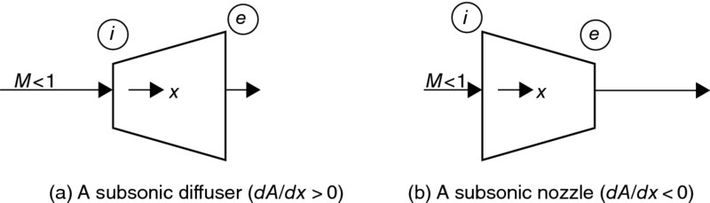
This equation relates area variation to speed variation for the subsonic and supersonic flows. Assuming a subsonic flow, the parenthesis involving Mach number becomes a negative quantity. Hence, an area increase in a duct, that is, dA > 0, results in du < 0, to make the signs of both sides of Equation 2.88b consistent. A negative du means flow deceleration. Hence, a subsonic diffuser requires a duct with dA/dx > 0. A subsonic nozzle with du > 0 demands dA < 0. These two duct geometries for a subsonic flow are shown in Figure 2.12.
FIGURE 2.12Area variations for a subsonic diffuser and a nozzle
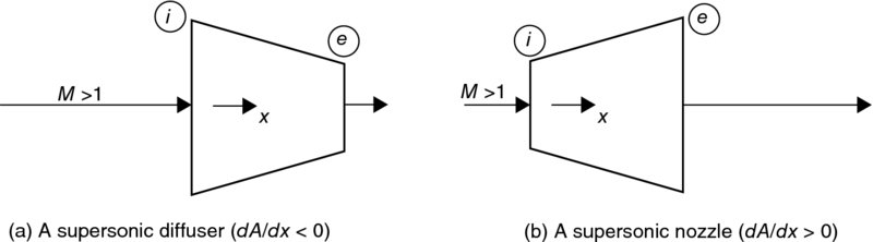
For a supersonic flow, the parenthesis that involves Mach number in Equation 2.88b is positive. Hence, an area increase results in flow acceleration and vice versa. These geometric relationships between area variation and flow speed for supersonic flow are shown in Figure 2.13.
FIGURE 2.13Area variations for a supersonic diffuser and nozzle
We note that the geometric requirements for a desired fluid acceleration or deceleration in a duct are opposite to each other in subsonic and supersonic flow regimes. This dual behavior is seen repeatedly in aerodynamics. We shall encounter several examples of this in this chapter.
2.9 Sonic Throat
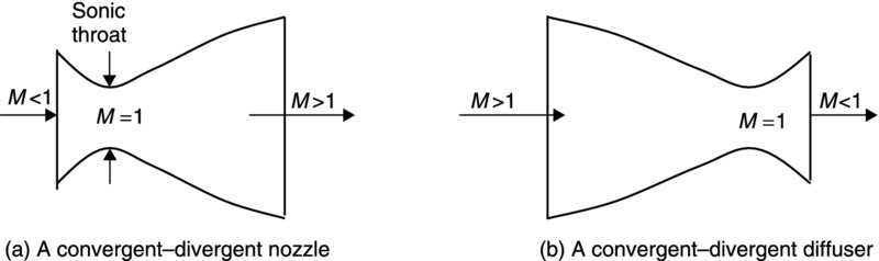
A unique flow condition separates the subsonic from supersonic flow. It is the sonic flow that marks the boundary between the two flows. In a subsonic flow, we learned that area reduction accelerates the gas and, ultimately, could reach a sonic state at the exit of the subsonic nozzle. A sonic flow may accelerate to supersonic Mach numbers if the area of the duct increases in the streamwise direction. This initial contraction and later expansion of the duct is capable of accelerating a subsonic flow to supersonic exit flow. This is called a convergent–divergent duct, with an internal throat, that is, the sonic throat. Conversely, a convergent–divergent duct with a supersonic entrance condition has the capability of decelerating the flow to subsonic exit conditions through a sonic throat. These duct geometries are shown in Figure 2.14.
FIGURE 2.14Convergent–divergent duct with an internal sonic throat
The sonic state where the gas speed and the local speed of sound are equal is distinguished with a asterisk. For example, the pressure at the sonic point is p* and the temperature is T*, the speed of sound is a*, and so on. Since the flow is isentropic throughout the duct, the stagnation pressure remains constant and as a consequence of adiabatic duct flow the stagnation temperature remains constant. By writing the stagnation temperature in terms of the local static temperature and local Mach number, we may relate the local static temperature to sonic temperature according to
(2.89)
Taken in ratio, the above equation yields
(2.90)
We may apply the isentropic relationship between temperature ratio and pressure ratio (Equation 2.24) to get an expression for p/p*.
(2.91)
From perfect gas law and the two expressions for temperature and pressure ratio, (2.90) and (2.91), we get an expression for the density ratio
(2.92)
The above expressions for the sonic ratios describe the properties of a section of the duct where flow Mach number is M to the flow properties at the sonic point. The mass flow rate balance between any section of the duct and the sonic throat yields an expression for the area ratio A/A*. First, let us write the continuity equation for a uniform flow in terms of the total gas properties, pt and Tt.
We replaced the density with speed of sound and pressure to get Equation 2.93a. Now, we may substitute the total pressure and temperature for the static pressure and temperature of Equation 2.93a and their respective functions of Mach number to get Equation 2.93b.
According to Equation 2.93b, we need the local flow area A, the local Mach number M, the local total pressure and temperature pt and Tt, respectively, and the type of gas, γ, R, to calculate the mass flow rate. The total temperature remains constant in adiabatic flows with no shaft work and the total pressure remains constant for isentropic flows with no shaft work, hence they are convenient parameters in Equation 2.93b. Since the mass flow rate between any two sections of a duct in steady flow has to be equal, Equation 2.93b is a Mach number–area relationship. We use the sonic flow area A*, with M = 1, to express a nondimensional area ratio.
(2.94)
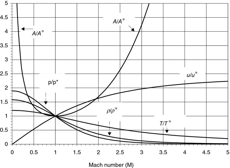
We may tabulate the functions p/p*, T/T*, and A/A* in addition to pt/p, Tt/T in an isentropic table for a specific gas, that is, γ = constant. Figure 2.15 shows the isentropic flow parameters as a function of Mach number for a diatomic gas, such as air.
FIGURE 2.15Isentropic flow parameters for a diatomic (calorically perfect) gas, γ = 1.4
At the minimum-area section, the ratio of mass flow rate to the cross-sectional area becomes maximum. Therefore, to demonstrate that M = 1 maximizes the mass flow per unit area, we differentiate the following equation and set it equal to zero,
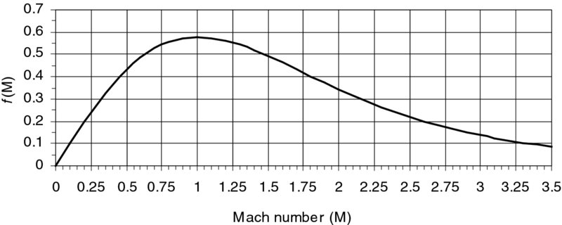
Equation 2.96 is identically satisfied by M = 1. We may also demonstrate this principle graphically by plotting the function f(M) (from Equation 2.93b):
Figure 2.16 is a graph of the nondimensional mass flow rate per unit area, that is, Equation 2.97.
FIGURE 2.16Nondimensional mass flow parameter variation with Mach number shows a sonic condition at the minimum-area section, i.e., the throat
2.10 Waves in Supersonic Flow
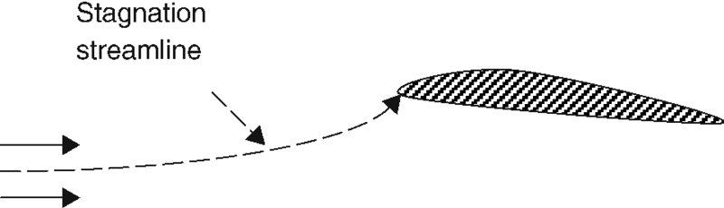
In a subsonic flow, a disturbance travels upstream to alert the flow of an upcoming object, say an airfoil. The streamlines in the flow make the necessary adjustments prior to reaching the obstacle to “make room” for the body that has a thickness. Figure 2.17 shows the phenomenon of “upwash” ahead of a subsonic wing, as evidence of subsonic flow adjustment before reaching the body.
FIGURE 2.17“Upwash” ahead of a subsonic wing section
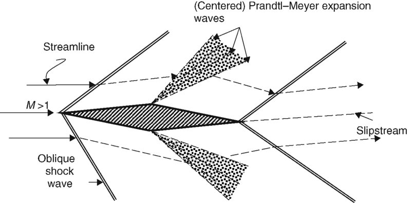
In contrast to a subsonic flow, the flowfield in a supersonic flow has to make adjustment for a body abruptly and within the zone of action. For small disturbances, the zone of action is the Mach cone, as shown in Figure 2.4. Larger disturbances, as in thick bodies or bodies at an angle of attack, create a system of compression and expansion waves that turn the supersonic flow around the body. The finite compression waves in aerodynamics are called shock waves due to their abrupt nature. A diamond airfoil in a supersonic flow shows the wave pattern about the body in Figure 2.18.
FIGURE 2.18Sketch of waves about a diamond airfoil at an angle of attack in supersonic flow
The attached oblique shocks at the leading edge turn the flow parallel to the surface and the expansion waves, known as the Prandtl–Meyer waves, cause the flow to turn at the airfoil shoulders. The trailing-edge waves turn the flow parallel to each other and the slipstream. The flow downstream of the tail waves, in general, is not parallel to the upstream flow. This is also in contrast to the subsonic flow that recovers the upstream flow direction further downstream of the trailing edge. The slipstream in supersonic flow allows for parallel flows and a continuous static pressure across the upper and lower parts of the trailing flowfield. It is the latter boundary condition that determines the slipstream inclination angle.
A special case of an oblique shock wave is the normal shock. This wave is normal to the flow and causes a sudden deceleration; static pressure, temperature, density, and entropy rise; Mach number and total pressure drop across the wave. We derive the jump conditions across a normal shock in the following section.
2.11 Normal Shocks
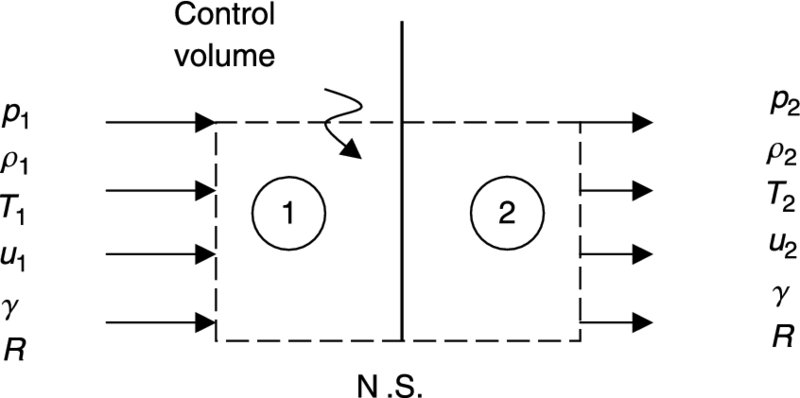
We apply the conservation principles to a normal shock flow, as shown in Figure 2.19. The shape of the control volume is chosen to simplify the applications of the conservation laws. The frame of reference is placed (with an observer) at the shock wave for a steady flow.
FIGURE 2.19Control volume for a normal shock (for an observer fixed at the shock)
To avoid writing the flow area of our arbitrary control volume, we choose it to be unity. The continuity equation of a steady flow through the control volume demands
(2.98)
The momentum equation in the x-direction is
(2.99a)
Now separating the flow conditions on the two sides of the shock, we get
Each side of Equation 2.99b is called fluid impulse per unit area, I/A. Since the flow area is constant across a normal shock, we conclude that impulse is conserved across the shock. We will return to impulse later in this chapter. By factoring the static pressure and introducing the speed of sound in Equation 2.99b, we get an alternative form of the conservation of momentum across the shock that involves Mach number and pressure, namely
(2.100)
The energy equation for an adiabatic flow with no shaft work demands the conservation of the total enthalpy, that is,
The essential unknowns in a normal shock flow are p2, ρ2, T2, and u2. The other unknowns are derivable from these basic parameters. For example, from the static temperature, T2, we calculate the local speed of sound, a2, and then the Mach number downstream of the shock, M2. Also, with the Mach number known, we may calculate the total pressure, pt2, and temperature, Tt2, downstream of a shock. The three conservation laws and an equation of state for the gas provide the four equations needed to solve for the four basic unknowns, that is, gas properties and the speed. These governing equations are coupled, however, and not immediately separable. We introduce the steps to the derivation of a normal shock flow in the following section.
We may relate the enthalpy to speed of sound, via Equation 2.61a, and derive alternative forms of the energy equation
(2.102a)
Divide through by u2, and multiply by (γ − 1), to get
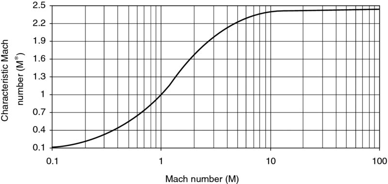
Here, we have introduced a new parameter M*, which is called the characteristic Mach number and has a definition
(2.103)
The characteristic Mach number is the ratio of local gas speed to the speed of sound at the sonic point. Hence, it is the ratio of two speeds at two different points in the flow. It is related to the local Mach number, M, through Equation 2.102b. If we solve for M*2 in terms of M2, we get the expression 2.104, which is plotted in Figure 2.20.
We note that for M < 1, M* is less than 1, for M = 1, M* is equal to 1, and for M > 1, M* is greater than 1. The characteristic Mach number is finite, however, as the Mach number M approaches infinity, M* approaches a finite value, that is,
(2.105)
For γ = 1.4, the limiting value of M* is .
FIGURE 2.20Variation of the characteristic Mach M*, with Mach number M, γ = 1.4
The momentum balance across the shock may be written as
From the continuity equation, we note that the product of density–velocity is a constant of motion, that is, ρ1u1 = ρ2u2, hence it may be cancelled from Equation 2.106. Also, we recognize that the ratio of static pressure to density is proportional to the speed of sound squared according to
Hence, the modified form of the momentum equation is
(2.107)
From energy Equation 2.101, we may replace the local speed of sound a by the local speed u and the speed of sound at the sonic point a* to get an equation in terms of the gas speeds across the shock and the speed of sound at the sonic point.
(2.108)
This equation simplifies to the Prandtl relation for a normal shock, that is,
(2.109)
Prandtl relation states that the product of gas speeds on two sides of a normal shock is a constant and that is the square of the speed of sound at the sonic point. This powerful expression relates the characteristic Mach number upstream and downstream of a normal shock via an inverse relationship, namely
(2.110)
We may also conclude from this equation that the flow downstream of a normal shock is subsonic, since the characteristic Mach number upstream of the shock is greater than 1. From Equation 2.104, we replace the characteristic Mach number by the local Mach number to get
(2.111a)
This equation contains as the only unknown and thus gives:
The downstream Mach number of a normal shock is finite even for M1 → ∞, which results in
(2.111c)
The density ratio across the shock is inversely proportional to the gas speed ratio via the continuity equation, which is related to the upstream Mach number according to
(2.112a)
We note that the density ratio is also finite as M1 → ∞, that is,
To derive the static pressure ratio across a shock, we start with the gas momentum equation. We may regroup the pressure and momentum terms in Equation 2.99b according to
(2.113)
Now, we may divide both sides by p1 and substitute for the density ratio from Equation 2.112, and simplify to get
(2.114)
From the perfect gas law, we establish the static temperature ratio across the shock in terms of the static pressure and density ratios in terms M1:
(2.115)
The stagnation pressure ratio across a normal shock may be written as the static pressure ratio and the function of local Mach numbers according to
(2.116)
The entropy rise across a shock is related to the stagnation pressure loss following Equation 2.73,
(2.117)
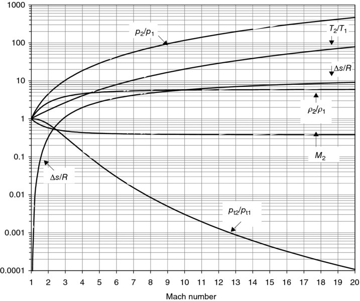
In summary, we established the downstream Mach number in terms of the upstream Mach number and all the jump conditions across a normal shock, that is, p2/p1, T2/T1, p2/p1, pt2/pt1, Δs/R, as well as identifying the constants of motion, namely:
Figure 2.21 shows the normal shock parameters for γ = 1.4 on a log-linear scale. Note that the density ratio as well as the Mach number downstream of the shock approach constant values as the Mach number increases.
FIGURE 2.21Normal shock parameters for a calorically perfect gas, γ = 1.4
2.12 Oblique Shocks
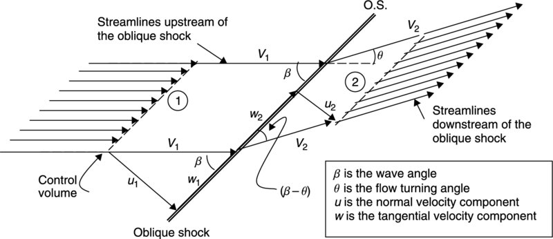
Compression Mach waves may coalesce to form an oblique shock wave. A normal shock is a special case of an oblique shock with a wave angle of 90°. Figure 2.22 shows a schematic drawing of an oblique shock flow with a representative streamline that abruptly changes direction across the shock. The shock wave angle with respect to upstream flow is called β and the flow-turning angle (again with respect to the upstream flow) is θ. A representative control volume is also shown in Figure 2.22. The flow is resolved into a normal and a tangential direction to the shock wave. The velocity components are u and w (normal and tangential to the shock wave front, respectively). Two velocity triangles are shown upstream and downstream of the shock with vertex angles β and (β − θ), respectively. The control volume is confined between a pair of streamlines and the entrance, and exit planes are parallel to the shock. We choose the area of the entrance and exit to be one for simplicity.
FIGURE 2.22Definition sketch of velocity components normal and parallel to an oblique shock, with the wave angle and flow turning angle definitions
To arrive at the shock jump conditions across the shock, we satisfy the conservation of mass, momentum normal and tangential to the shock, and the energy across the oblique shock. The continuity equation demands
(2.118)
The conservation of normal momentum requires the momentum change normal to the shock to be balanced by the fluid forces acting in the normal direction on the control volume. The only forces acting normal to the shock are the pressure forces acting on the entrance and the exit planes of the control surface.
(2.119)
The conservation of momentum along the shock front, that is, tangential to the shock, requires
The net pressure forces in the tangential direction are zero, hence the tangential momentum is conserved. We may cancel the continuity portion of Equation 2.120 to arrive at the simple result of the conservation of tangential velocity across an oblique shock, namely
(2.121)
The energy equation demands the conservation of total enthalpy, therefore
(2.122)
Since the tangential velocity is conserved across the shock the energy equation is simplified to
(2.123)
Now, we note that the conservation equations normal to the shock take on the exact form of the normal shock equations that we solved earlier to arrive at the shock jump conditions. Consequently, all the jump conditions across an oblique shock are established uniquely by the normal component of the flow to the oblique shock, that is, M1n.
From the wave angle β, we get
(2.124)
The normal shock relation Equation 2.111b establishes the normal component of the Mach number downstream of an oblique shock, according to
(2.125)
From the velocity triangle downstream of the oblique shock, we have
To summarize, an oblique shock jump conditions are established by the normal component of the flow and the downstream Mach number follows Equation 2.126. To establish a relationship between the flow turning angle and the oblique shock wave angle, we use the velocity triangles upstream and downstream of the shock,
(2.127)
(2.128)
The ratio of these two equations relates the angles and the normal velocity ratio according to
Now substituting for the density ratio from the normal shock relations, we get
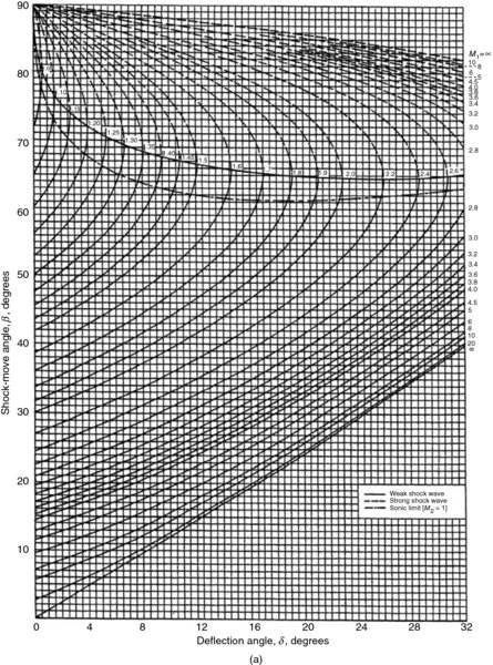
Expression 2.129 is called “θ–β–M” equation and a graph of the oblique shock angle versus the turning angle is plotted for a constant upstream Mach number to create oblique shock charts. In the limit of zero turning angle, that is, as θ → 0,
which identifies an infinitesimal strength shock wave as a Mach wave, and the second is β = 90°, which identifies a normal shock as the strongest oblique shock. Thus, the weakest oblique shock is a Mach wave and the strongest oblique shock is a normal shock. Since the strength of the wave depends on M · sin βs, an oblique shock wave angle is larger than the Mach angle, that is,
(2.132)
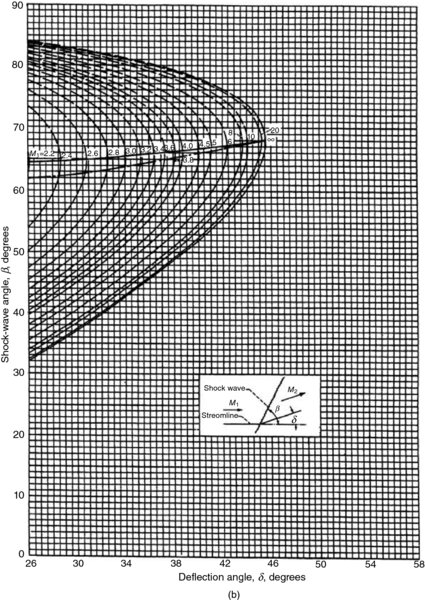
Figure 2.23 is a graph of Equation 2.129 with Mach number as a running parameter (from NACA Report 1135, 1953). There are two solutions for the wave angle β for each turning angle θ. The high wave angle is referred to as the strong solution, and the lower wave angle is called the weak solution. A continuous line and a broken line distinguish the weak and strong solutions in Figure 2.23, respectively. Also, there is a maximum turning angle, θmax, for any supersonic Mach number. For example, a Mach 2 flow can turn only ∼ 23° via an attached plane oblique shock wave. For higher turning angles than θmax, a detached shock will form upstream of the body. This shock, due to its shape, is referred to as the bow shock.
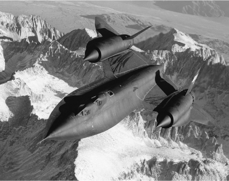
The SR-71 at Mach 3+ is a marvel in supersonic aerodynamic and propulsion system design. Courtesy of NASA
FIGURE 2.23(a) The plane oblique shock chart for γ = 1.4 (from NACA Report 1135, 1953); (b) The plane oblique shock chart continued (from NACA Report 1135, 1953)
2.13 Conical Shocks
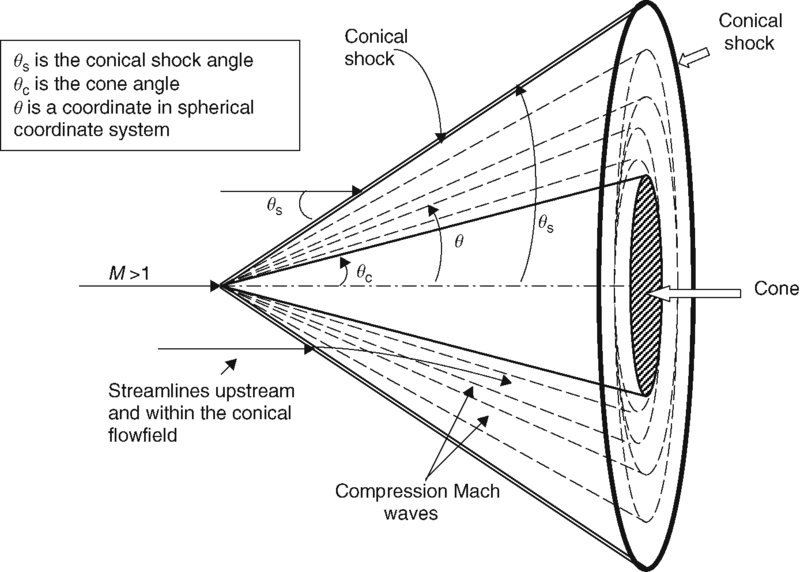
A cone in supersonic flow creates a conical shock. In the case of zero angle of attack, the flowfield is axisymmetric and the cone axis and the conical shock axis coincide. The jump conditions at the shock are, however, established by the (local) normal component of Mach number to the shock front. The flowfield behind a conical shock continues to vary from the shock surface to the cone surface. In a plane oblique shock case, the flowfield undergoes a single jump at the shock and then its flow properties remain constant. The mechanism for a continuous change behind a conical shock is the compression Mach waves emanating from the cone vertex. These are the rays along which flow properties remain constant. Note that an axisymmetric conical shock flow lacks a length scale and hence θ becomes the only variable of the problem. Figure 2.24 shows a definition sketch of an axisymmetric conical shock flow.
FIGURE 2.24Definition sketch of a conical shock flowfield
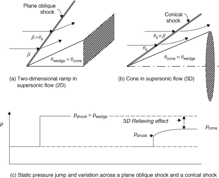
All the jump conditions across the conical shock depend on M · sinθs as we derived earlier in this section. The flow properties downstream of the shock, for example, p, T, ρ, V, are a function of the conical angle θ, that is, p(θ), etc. Therefore, all the rays emanating from the cone vertex have different flow properties. The cone surface is a ray itself and thus experiences constant flow properties, such as pressure, temperature, density, velocity, and Mach number. The streamlines downstream of a conical shock continue to turn in their interaction with the compression Mach waves. The flowfield downstream of the conical shock remains reversible, however, as the compression Mach waves are each of infinitesimal strength. The flowfield downstream of an axisymmetric conical shock is irrotational since the shock is straight, hence of constant strength. We apply conservation principles to arrive at the detail flowfield downstream of a conical shock. In addition, we utilize the irrotationality condition to numerically integrate the governing conical flowfield equation, known as the Taylor–Maccoll equation. A cone of semivertex angle θc would create a conical shock wave of angle θs, which is smaller than a corresponding plane oblique shock on a two-dimensional ramp of the same vertex angle. This results in a weaker shock in three-dimensional space as compared with a corresponding two-dimensional space. This important flow behavior is referred to as the 3D relieving effect in aerodynamics. Figure 2.25 shows a two-dimensional compression ramp and a conical ramp of equal vertex angle in supersonic flow.
FIGURE 2.25Three-dimensional relieving effect on a cone
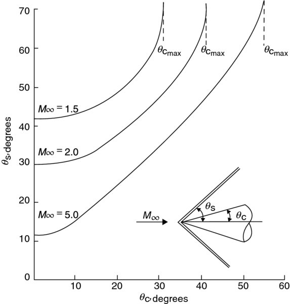
A conical shock chart for three Mach numbers is shown in Figure 2.26 (from Anderson, 2003). This figure contains only the weak solution. Note that the maximum turning angle for a given Mach number is larger for a cone than a two-dimensional ramp of the same nose angle. This, too, is related to the well-known 3D relieving effect.
FIGURE 2.26Conical shock chart for a calorically perfect gas, γ = 1.4. Source: Anderson 2003, Fig. 10.5, p. 373. Reproduced with permission from McGraw Hill
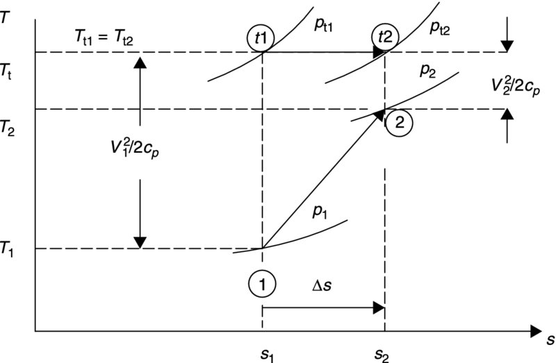
Finally, we graph a shock wave static and stagnation states on a T–s diagram (Figure 2.27). All shocks are irreversible and, hence, suffer an entropy rise, as graphically demonstrated in Figure 2.27. The static path connects points 1 and 2 across the shock wave. The stagnation path connects “tl” to “t2.” The constant-pressure lines indicate a static pressure rise and a stagnation pressure drop between the two sides of a shock. The static temperature rises and the stagnation temperature remains constant (assuming cp is constant as in a calorically perfect gas). We also note a drop in the kinetic energy of the gas, which is converted into heat through viscous dissipation within the shock. Shocks are generally thin and are of the order of the mean free path of the molecules in the gas. Thus, shocks are often modeled as having a zero thickness, unless the gas is in near vacuum of upper atmosphere where the mean free path is of the order of centimeters.
FIGURE 2.27Static and stagnation states of a (calorically perfect) gas across a shock wave


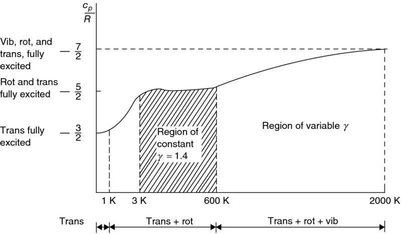
 FIGURE 2.1 Temperature dependence of specific heat for a diatomic gas. Source: Anderson 2003, Fig. 16.11, p. 613. Reproduced with permission from McGraw Hill