
11.3.3 Off-Design Analysis of a Separate-Flow Turbofan (Two-Spool) Engine
We will approach the off-design analysis problem of separate-flow turbofan engines the same way we did in the turbojet problem, that is, we assume the first nozzle choking stations in the turbine as well as the exhaust nozzle throat in off-design engine operation. Then we set the mass flow rates between the choked stations equal to each other and establish the constants of gas turbine engine operation.
Figure 11.12 shows a definition sketch of a two-spool separate-flow turbofan engine. The fan is driven by the low-pressure turbine (LPT), and the high-pressure compressor (HPC) is driven by the high-pressure turbine (HPT). Again, we assume that the first turbine nozzles of the HPT and LPT are choked at design point and remain choked in off-design operation, that is,

 FIGURE 11.12 Two-spool separate-flow turbofan engine with choked convergent nozzles
The second assumption deals with the exhaust nozzle throats, that is,
The known design parameters for this turbofan engine are
| 1. Design flight condition | M0, p0, T0 |
| 2. Design compressor and fan pressure ratios | πc, πf |
| 3. Design bypass ratio | α |
| 4. Ideal heating value of the fuel | QR |
| 5. Design turbine inlet temperature | Tt4 (or expressed as τλ) |
| 6. Design component efficiencies | πd, ec, ef, πb, ηb, et, ηm, πn, πnf, p8/p0, p18/p0 |
| 7. Gas properties at design point | γc, cpc, γt, cpt |
| 8. Design choked stations | M4 = M4.5 = M8 = M18 = 1.0 |
In off-design condition, we may have a different throttle setting and fly at a different altitude Mach number, that is, we subject the turbofan engine to
- Off-design flight conditions (specified) M0, p0, T0
- Off-design turbine inlet temperature (specified) Tt4 or τλ
And off-design inlet losses.
The primary unknowns, in the off-design operation, are three cycle parameters, namely,
- πc, O–D
- πf, O–D
- αO–D
The mass flow rates between the stations 4.5 and the nozzle throat are nearly the same, therefore,

Using similar arguments as in the turbojet section, for example, constant areas, constant gas properties, and so on, we conclude that,
or assuming the same polytropic efficiency that relates pressure and temperature ratios in the turbine, we conclude that the first constant of operation in our separate-flow turbofan engine is
Now let us consider the mass flow rates between two other stations, namely, station 4 and 4.5, that is,

For fixed area turbines, A4 and A4.5 remain constant, that is, they are not adjustable, and assuming the gas properties do not appreciably change between the on- and off-design conditions, we may conclude that the second constant of engine operation is
and similarly, assuming constant etH between on- and off-designs, we conclude that
Note that the combination of Equations 11.53b and 11.54b results in the constant overall expansion across the turbine, that is,
The fan nozzle is assumed to remain choked in off-design as well as on-design operation, which states that its mass flow rate is

The main nozzle mass flow rate may be written as

Taking the ratio of the two mass flow rates in Equations 11.55 and 11.56 and assuming the gas properties and the flow nozzle throat areas do not change between the on- and off-designs, we get

We may divide the numerator and denominator by pt2/(Tt2)1/2 to get

Note that all the constants were combined in the coefficient in front of the RHS, for example, turbine pressure ratio or temperature ratio, which do not change were lumped in the constant of the above equation. Since the turbine expansion parameters τt and πt remain constant in off-design, we may further simplify Equation 11.57 to get

The last equation, that is, Equation 11.58 constitutes the third constant of turbofan operation, within the approximations that we introduced. We use these three constants of operation between the on-and off-design modes to establish the three unknowns at off-design, namely, the fan and the compressor pressure ratio as well as the bypass ratio.
Off-design analysis
The power balance between the HPT and HPC yields
We may divide both sides by Tt2 to get the nondimensional expression
Note that this has only two unknowns and they are τcH and τf since we specify the throttle setting at off-design, Tt4 (or τλ) as well as flight Mach number produces τr information. We may cast Equation 11.59 as
The power balance between the fan and the LPT yields
We note that the RHS of the above equation is completely known, either from the design point calculations as in τtH and τtL or from the off-design throttle setting Tt4. The LHS of Equation 11.61 contains two unknowns, namely, the off-design bypass ratio and the off-design fan temperature ratio. The Equation 11.61 simplifies to
Now, we use the third constant, that is, Equation 11.58, to establish a third equation involving the three unknowns, α and τf, and πcH at off-design.
Is there a closed form solution for the three unknowns in terms of the three constants C1, C2, and C3? The answer is no, since these equations are coupled and involve unknowns with the following exponent:
Off-design solution strategy
From the on-design cycle analysis, calculate the three constants, C1, C2, and C3. Then solve Equations 11.60, 11.62 and 11.63 iteratively to arrive at the unknowns α, τcH, and τf. We may eliminate the bypass ratio α from Equations 11.62 and 11.63, and after some minor simplification, we get
From Equation 11.60, we isolate τf, to get
We introduce expression 11.66 into Equation 11.65 and replace pressure ratio by the temperature ratio via Equation 11.64 will result in a one equation, one unknown expression,

Finally, we need to iterate for τcH in Equation 11.67. Then introducing it in Equation 11.66 yields τf and substituting them in Equation 11.63, we get the off-design bypass ratio α.
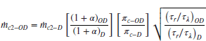
The corrected mass flow rate at off-design is related to the design value via:

Where πc is the engine overall pressure ratio, namely πf.πcH.
To demonstrate the methodology, we solve an example.
11.4 Unchoked Nozzles and Other Off-Design Iteration Strategies
Let us reexamine the assumptions that we made in component matching and engine off-design analysis, in particular, choked flow condition at stations: 4, 4.5, and 8, that is, the HPT entrance, the LPT entrance, and the exhaust nozzle throat. These choked stations simplified our solution methodology, as the corrected mass flow rate in those stations remained fixed. However, what if those stations were not choked, that is, what if M4 ≠ 1.0, M4.5 ≠ 1, and M8 ≠ 1, in some off-design operations? How do we know our assumption was correct?
11.4.1 Unchoked Exhaust Nozzle
We may start our off-design analysis with the assumption of choked stations at 4, 4.5, and 8, as described earlier. With these assumptions, we may calculate the missing off-design cycle parameters, namely, the compressor and fan pressure ratios and bypass ratio (if a turbofan engine). Then, we can march through the engine and calculate all the total pressures and temperatures in the engine including pt9 if a convergent–divergent (C–D) nozzle or pt8 if the nozzle was convergent. Now, we apply the nozzle-choking criterion, or what we called critical nozzle pressure ratio (NPR)crit, for a choked throat in a C–D nozzle we must have
For a choked throat in a convergent nozzle we must have
With these conditions met, we had made correct assumptions (i.e., M8 = 1.0). Otherwise, the nozzle throat Mach number is less than 1 and its value is

With a reduced Mach number at the throat, the corrected mass flow rate through the nozzle throat drops.
If we write the corrected mass flow rate at the turbine inlet as

And take the ratio of the two corrected mass flow rates while ignoring variation of gas constants, we get
Note that although the corrected mass flow rate at 8 has dropped (to below critical), it may not have caused the turbine nozzle to unchoke. Therefore, we continue with the assumption that turbine nozzle is choked, that is, M4 = 1.0 or ![]() , and our new turbine expansion equation becomes
, and our new turbine expansion equation becomes
Compare this equation with Equation 11.45, when we had made the assumption of choked flow at 8, that is,
Equation 11.74 indicates that turbine expansion is no longer constant when the throat unchokes, rather it is inversely proportional to the nozzle corrected mass flow rate at the nozzle throat. A reduction in the corrected mass flow rate at the nozzle throat then causes the turbine pressure ratio πt or backpressure pt5 to increase, which in turn reduces the turbine shaft power, which causes the compressor pressure ratio and mass flow rate to drop, in a domino effect.
In summary, the iteration strategy for an unchoked exhaust nozzle throat is
- Calculate the nozzle throat Mach number from Equation 11.70 (using pt8/p0 from round 1)
- Calculate the corrected mass flow rate at 8 from Equation 11.71
- Calculate a new turbine expansion parameter from Equation 11.74
- Calculate the new cycle pressure ratio, bypass ratio, fan pressure ratio, and so on
- Calculate the new pt8 /p0 from the new cycle parameters
-
Calculate the new nozzle throat Mach number from Equation 11.70 (from round 2)
- Compare the two throat Mach numbers (from round 1 and 2)
- Repeat the process until the two nozzle throat Mach numbers are within say ∼1%.
11.4.2 Unchoked Turbine Nozzle
In certain low mass flow rate conditions, it is possible for the turbine nozzle to operate in an unchoked mode. Typically, an inverse turbine pressure ratio (1/πt) of ∼2 is the boundary between choked and unchoked turbine operation at low mass flow rates. The following rule of thumb is thus of interest:
When the turbine unchokes (mainly due to low mass flow rate conditions), its corrected mass flow rate at station 4 drops (to below critical corresponding to Mach 1 condition). The new turbine expansion parameter, from Equation 11.73 then follows the more general rule of

Here we have fixed the exhaust nozzle corrected flow ![]() as in the previous section, but we now have to iterate on the turbine corrected flow
as in the previous section, but we now have to iterate on the turbine corrected flow ![]() . The strategy here is that for a given exhaust nozzle corrected mass flow rate
. The strategy here is that for a given exhaust nozzle corrected mass flow rate ![]() that we calculate from Equation 11.71, we assume a new (and lower)
that we calculate from Equation 11.71, we assume a new (and lower) ![]() , and then using Equation 11.75, we calculate a new turbine expansion parameter. The new cycle parameters at off-design are then calculated, which lead to a test of M8 as in step #7 in the iteration strategy of Section 11.4.1.
, and then using Equation 11.75, we calculate a new turbine expansion parameter. The new cycle parameters at off-design are then calculated, which lead to a test of M8 as in step #7 in the iteration strategy of Section 11.4.1.
11.4.3 Turbine Efficiency at Off-Design
So far we have considered the turbine pressure and temperature ratios that are related via constant polytropic efficiency et according to
Alternatively, we have turbine adiabatic efficiency ηt that connects the turbine pressure and temperature ratios following
In reality, turbine efficiency, either et or ηt, changes with operating condition and the turbine expansion parameter that was kept constant between the on- and off-design was
From our design analysis, we determine the RHS of the above equation (constant C1), then we have two equations and two unknowns, for τt and πt, if we know (or can estimate) the off-design efficiency ηt. For example, we have to numerically solve the following equation for τt.
11.4.4 Variable Gas Properties
Up to this point in our analysis, we have prescribed gas properties at both design and off-design conditions. In the off-design analysis, the compressor pressure ratio and, therefore, its exit temperature Tt3 are both unknown. Since for a thermally perfect gas we have
we need to recalculate all gas properties based on our cycle temperatures and, in fact, we have to include the effect of fuel-to-air ratio on the gas constants after the burner. Based on the recalculated gas properties, we have to repeat the cycle analysis and continue the loop until certain level of accuracy (in, for example, τt) is achieved. Every one of these steps represents a higher level of refinement in engine performance simulation. The complexities of the iteration loops and gas modeling have prompted the creation of computer codes. One example is the NNEP, which stands for Navy/NASA Engine Program, which also interfaces with CEC (complex chemical equilibrium composition).
11.5 Principles of Engine Performance Testing
Full-scale (prototype) engine performance testing is of vital importance to propulsion industry before a commitment can be made for their production. Prior to full engine performance testing, each component is extensively tested in component test rigs. For example, a compressor test rig tests and develops the compressor performance map, including its stall and choke boundaries. The impact of inlet flow distortion on compressor stall characteristics/deterioration would also be assessed. Once the component performance maps are completely determined, the full-scale engine testing program begins. Some of the key parameters of interest in an engine performance testing are shown in the following list:
- Engine thrust
- Engine air mass flow rate
- Engine fuel consumption
- Engine controls effectiveness, for example, in acceleration/deceleration and engine stability
- Engine, that is, shaft, vibration levels
- Engine noise and exhaust gas emissions.
The instrumentation used in engine performance testing is calibrated to measure the steady state and transient characteristics of pressure (via low and high frequency response pressure transducers), temperature (via thermocouples), shaft speed (via magnetic transducer or tacho-generator), shaft vibration level (via accelerometer), turbomachinery blade tip clearance (via capacitive sensors or optical probes), air flow (via instrumented bellmouth or venturi meter), fuel flow (via flow meters) and thrust (via load cells). The location of measurement stations and the respective parameters in a single-spool turbojet engine are shown in Figure 11.13.

FIGURE 11.13 Schematic drawing of an instrumented turbojet engine in an open-air testing facility
The air temperature and pressure, p0 and T0, are used to correct for the nonstandard testing conditions. Namely, engine thrust, F, air mass flow rate and thrust-specific fuel consumption, TSFC, are first corrected according to:

and then expressed as a function of corrected shaft speed
The air humidity impacts gas properties, namely its density, ρ, the ratio of specific heats, γ, and gas constant, R. Since water vapor has a molecular weight of 18 as compared to 29 for air, their mixture, that is, humidity in atmospheric air, lowers the ambient density. For the same reason, the gas constant, R, cp and cv for humid air are higher than for dry air. Also, since the humid air is partially composed of a tri-atomic gas (H2O) versus air, which is primarily composed of diatomic gas (N2, O2), the ratio of specific heats, γ, is lower for humid air. Consequently, the mass flow rate and, thus, thrust need to be corrected for the effect of humidity in atmospheric air.
The effect of wind speed and direction in open air installations is in creating ram drag and side-force, which impacts the accuracy of gross thrust measurement. Consequently, only head wind of less than 10 knots is the accepted limit in open-air testing practice. The engine noise is measured by an array of microphones placed at various distances and angular positions with respect to the engine centerline. The exhaust emissions (UHC, CO, NOx, CO2 and H2O) are measured by gas analyzer probe (mass spectrometer), which is inserted in the exhaust nozzle and measures the mole fractions of the constituent gas.
Engine performance testing is conducted in different environments and facilities. The following group represents the ground facilities:
- open-air ground testing facility (GTF)
- engine test cell
- altitude testing facility (ATF)
- ram air facility.
In addition to these, there are certification facilities for icing and bird ingestion that are also conducted in ground test facilities. Finally, flying test bed aircraft are used to calibrate the engine thrust and aircraft drag data in flight and correlate the flight and ground test data. The consistent and corrected set of data is then used in the development of the control laws for the engine, namely through the development of the full-authority digital electronic controller (FADEC). Figures 11.14–11.17 show ground test facilities and flight test bed aircraft (courtesy of Pratt & Whitney). For additional reading on engine testing and thrust determination, Abernethy and Roberts (1986) and Covert et al. (1985) should be consulted.

FIGURE 11.14 PW1524G engine in ground testing at the Pratt & Whitney West Palm Beach, FL, test facility. Source: Reproduced by permission of United Technologies Corporation, Pratt & Whitney
FIGURE 11.15 PW1524G engine conducting natural icing tests at the GLACIER facility in Thompson, Manitoba, Canada. Source: Reproduced by permission of United Technologies Corporation, Pratt & Whitney

FIGURE 11.16 PW1217G flight testing on one of the two P&W B747SP Flying Test Beds. Source: Reproduced by permission of United Technologies Corporation, Pratt & Whitney

FIGURE 11.17 PW1133G first flight on P&W B747SP Flying Test Bed. Source: Reproduced by permission of United Technologies Corporation, Pratt & Whitney
11.5.1 Force of Inlet Bellmouth on Engine Thrust Stand
An inlet bellmouth is a bell-shaped converging duct (i.e., a nozzle) that provides for smooth flow acceleration into an airbreathing engine on a static thrust stand (Figure 11.18). The bellmouth is characterized by its contraction area ratio, A1/A2, and its length ratios, L1/D2 and L2/D2. The length ratio, L1/D2, in the contraction section and the length of the constant-area throat section, L2/D2, provide for a uniform, low-distortion flow into the engine. The test cell pressure, temperature and humidity are recorded prior to engine testing. Since the engine is stationary, the test cell pressure and temperature serve as the stagnation, or total, values of pressure and temperature respectively for the engine.

FIGURE 11.18 Inlet bellmouth and a jet engine on a static thrust stand in a ground testing facility
11.5.1.1 Bellmouth Instrumentation
The static pressure is measured at the bellmouth throat at four azimuthal locations, as shown in Figure 11.19. A certain amount of asymmetry in the flow is to be expected, even in the most controlled environment of axisymmetric installations. The throat pressure is the average of the four measured wall static pressures. The average throat pressure is used to calculate the air mass flow rate into the engine. In addition to throat static pressure measurements, the bellmouth may be equipped with other wall static pressure taps that are distributed both axially and azimuthally from the lip to the throat. In essence the static pressure distribution on the bellmouth can be used to estimate the resultant axial pressure force on the thrust stand (exerted by the bellmouth).
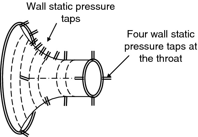
FIGURE 11.19 Schematic drawing of an inlet bellmouth with its wall static pressure taps
11.5.1.2 The Effect of Fluid Viscosity
The effect of fluid viscosity is to form boundary layer on the bellmouth wall. As the fluid is accelerating along the wall, the boundary layer is facing a “favorable” pressure gradient and thus remains attached (and thin). The boundary layer formation creates blockage and an effective flow area as well as resulting in a reduction in total pressure. The boundary layer displacement thickness at the bellmouth exit, which causes a reduction in the flow area (in A2), is described by a discharge coefficient, Cd2; typically, 0.990–0.995 is a reasonable approximation.
11.5.1.3 The Force of Inlet Bellmouth on Engine Thrust Stand
We may numerically integrate the measured wall static pressure distribution on the bellmouth to get the axial force due to pressure. According to the pressure difference on the outer and inner walls (Figure 11.20a), we can write

FIGURE 11.20 Pressure distribution on the inner and outer wall of a bellmouth
Note that the integrand, that is, (p–p0) in Equation 11.81 is negative and dAy is also negative (for a converging duct), which produces an axial force in the –x direction. Therefore, we conclude that the bellmouth experiences a thrust force and thus “pulls” on the thrust stand.
The flow acceleration inside the bellmouth causes a static pressure drop whereas the test cell static pressure acts on the outside wall, as shown in Figure 11.20. The static pressure and velocity distribution are nonuniform at the bellmouth inlet (as shown in Figure 11.21) due to flow curvature near the convex wall.

FIGURE 11.21 The bellmouth inlet flow nonuniformity shows overspeed and suction near the convex wall ( is the mass-averaged inlet velocity and
  is the average static pressure at the bellmouth inlet)
Based on (four) measured static pressures at 2, we define an average static pressure,
The ideal exit Mach number, based on the average throat static pressure is:

Assuming an adiabatic flow inside the bellmouth, the test cell static temperature is the stagnation temperature inside the bellmouth, namely at its exit, that is, and the static temperature at 2 is thus
The speed of sound and the average flow speed at the bellmouth exit are respectively:
From the average pressure and temperature at 2, we use perfect gas law to get the fluid density at 2, that is,
Note that the assumption of incompressible flow could have been made, since the flow Mach numbers inside the bellmouth are small. The mass flow rate through the bellmouth may now be calculated based on exit values of fluid density, velocity and “effective” flow area, A2eff, which is related to the discharge coefficient that was introduced earlier, Cd2,
In general, the flow speed in the bellmouth is in low subsonic range, which makes the assumption of incompressible flow reasonable. The one-dimensional gas speed at the inlet follows the continuity equation and assuming constant density, that is,
The use of the Bernoulli equation at the bellmouth inlet gives a one-dimensional estimation of p1, namely
The one-dimensional momentum balance in the x-direction on the captured streamtube (control volume), based on the fluid impulse, gives an estimate of the bellmouth internal axial force that acts on the fluid, that is,
The bellmouth (inner wall) feels an equal and opposite force of that felt by the fluid, that is,
The bellmouth outer wall is soaked in ambient static pressure, p0, which integrates into the following axial force in the –x-direction, that is, the bellmouth external axial force,
Therefore, the net force acting on the bellmouth in the x-direction is the sum of internal and external components, namely
We have either measured or calculated all the terms in Equation 11.94, thus we may estimate the axial force that is introduced by the installation of the inlet bellmouth on the thrust stand. Since the value of the bellmouth axial force will be negative, we conclude that ‘the bellmouth is pulling on the thrust stand, that is, it produces its own thrust. The load cell measures the entire “pull” on the frame, which has a contribution from the bellmouth as well. The engine thrust measurement using the load cell is thus to be corrected for the bellmouth-induced thrust.
A closer examination of Figure 11.20b also reveals that the integral of pressure on the bellmouth will produce a force in the thrust (i.e., –x) direction.
The bellmouth axial force may be nondimensionalized by the product of test cell static pressure, p0, and the bellmouth exit area, A2, that is,
11.6 Summary
The purpose of this chapter was to integrate our individual component studies into a complete propulsion system. We asked and answered the question of how an aircraft gas turbine engine (that was designed for certain operating conditions) behaved in off-design. We started with a review of the five corrected parameters in an engine:


- Fc ≡ F/δ0

We learned about the individual component interaction in a steady-state mode of operation. The conservation principles of mass and energy provided the link, that is, the match, between the components. In case the compressor and turbine performance maps were available, we used them to calculate the gas generator pumping characteristics for a given throttle setting. Pumping characteristics are
- the corrected air/flow rate

- the pressure ratio pt5 /pt2
- the temperature ratio Tt5/Tt2
- the fuel flow parameter fQRηb/cpTt2 or the corrected fuel flow rate

If the component performance maps were not available, we relied on the persistence of certain choking stations in the engine (as in stations 4 and 8 in a single-spool engine and 4, 4.5, and 8 in a two-spool engine) in on- and off-designs to calculate the off-design performance of the engine. The highest level of simplifications, as in constant component efficiencies, gas properties, negligible fuel-to-air ratio variation, and so on, resulted in a constant turbine expansion parameter in a single-spool turbojet engine
between the on- and off-designs. We used the same principles in a two-spool turbofan engine that resulted in three constants between the on- and off-design turbine expansion parameters and one involving bypass ratio
In the case that the exhaust nozzle throat was unchoked, the corrected mass flow rate at the nozzle throat was reduced and the turbine expansion parameter τt was no longer constant, that is,
An iteration strategy to arrive at a consistent operating condition of the engine in off-design was outlined in Section 11.4.1. Other iteration strategies were presented for unchoked turbine and variable gas properties.
The most critical and perhaps interesting part of the engine component matching is in the study of engine transients and unsteady interactions. For example, stall and surge are unsteady behavior of the compression–combustor system. The phenomenon of inlet unstart and upstream propagation of “hammer shock” finds its root in supersonic mixed-compression inlet instability. External compression inlets may initiate “buzz” instability and subsequent compressor stall. The acceleration and deceleration paths (i.e., spool up and down) in an engine are transients that too may cause compressor instability. In general, the question that we need to ask is what happens if we disturb the steady state? Would the oscillations in the system decay or grow? What is the impact of the rate of change that we introduce in the dynamic system, as in the rate of fuel addition, spool up or spool down, or rapid actuation of (stator) blades? Kerrebrock’s paper (1977) on small disturbance theory examines the growth/decay characteristics of pressure, entropy, and vorticity perturbations in swirling flows in turbomachinery. Schobeiri (2005) has treated the time-dependent, dynamic performance of turbomachinery and gas turbine systems extensively in his book.
Finally, there are many aircraft engine simulation codes, for example, NNEP that provide for an accurate estimation of the engine performance characteristics over a wide operating range of the engine/aircraft. Also, a major new initiative on propulsion system simulation is NASA-Glenn’s “Numerical Propulsion System Simulation” (NPSS) Program (Lytle, 1999) that promises to bring high fidelity to fully three-dimensional transient simulation of complex aircraft engine configurations.
The principles that we learned in this chapter help us to (1) produce engine off-design performance for preliminary design purposes, (2) use compressor and turbine performance maps to calculate the gas generator pumping characteristics, and (3) understand and interpret the results of engine simulation codes, if they are available and used.
Additional references (e.g., 2, 3, 5–7, 9–12, and 15–19) on gas turbine and aircraft propulsion compliment the subject of this chapter and are recommended for further reading.
References
- Abernethy, R.B. and Roberts, J.H., In-Flight Thrust Determination and Uncertainty, SAE Special Publication 64, 1986.
- Archer, R.D. and Saarlas, M., An Introduction of Aerospace Propulsion, Prentice Hall, New York, 1998.
- Bathie, W., Fundamentals of Gas Turbines, 2nd edition, John Wiley & Sons, Inc., New York, 1995.
- Covert, E.E., James, C.R., Richey, G.K., and Rooney, E.C., Thrust and Drag: Its Prediction and Verification, AIAA Progress Series, Vol. 98, AIAA, New York, 1985.
- Cumpsty, N., Jet Propulsion: A Simple Guide to the Aerodynamic and Thermodynamic Design and Performance of Jet Engines, 2nd edition, Cambridge University Press, Cambridge, UK, 2003.
- Flack, R.D., Fundamentals of Jet Propulsion with Applications, Cambridge University Press, Cambridge, UK, 2005.
- Gordon, S. and McBride, B.J., “Computer Program for Computation of Complex Chemical Equilibrium Compositions, Rocket Performance, Incident and Reflected Shocks, and Chapman-Jouguet Detonations, ” NASA SP-273, 1976.
- Gordon, S. and McBride, B.J., “Computer Program for Calculation of Complex Chemical Equilibrium Compositions and Applications I. Ananlysis”, NASA RP-1311, 1994.
- Heiser, W.H., Pratt, D.T., Daley, D.H., and Mehta, U.B., Hypersonic Airbreathing Propulsion, AIAA, Washington, DC, 1993.
- Hesse, W.J. and Mumford, N.V.S., Jet Propulsion for Aerospace Applications, 2nd edition, Pittman Publishing Corporation, New York, 1964.
- Hill, P.G. and Peterson, C.R., Mechanics and Thermodynamics of Propulsion, 2nd edition, Addison-Wesley, Reading, MA, 1992.
- Kerrebrock, J.L., Aircraft Engines and Gas Turbines, 2nd edition, MIT Press, Cambridge, MA, 1992.
- Kerrebrock, J.L., “Small Disturbances in Turbomachine Annuli with Swirl, ” AIAA Journal, Vol. 15, June 1977, pp. 794–803.
- Lytle, J.K., “The Numerical Propulsion System Simulation: A Multidisciplinary Design System for Aerospace Vehicles, ” NASA TM-1999-209194.
- Mattingly, J.D., Elements of Gas Turbine Propulsion, McGraw-Hill, New York, 1996.
- Mattingly, J.D., Heiser, W.H., and Pratt, D.T., Aircraft Engine Design, 2nd edition, AIAA, Washington, DC, 2002.
- Oates, G.C., Aerothermodynamics of Gas Turbine and Rocket Propulsion, AIAA, Washington, DC, 1988.
- Schobeiri, M.T., Turbomachinery Performance and Flow Physics, Springer Verlag, New York, 2005.
- Shepherd, D.G., Aerospace Propulsion, American Elsevier Publication, New York, 1972.
Problems
- 11.1 In aturbojet engine, the compressor face total pressure and temperature are 112 kPa and 268 K, respectively. The shaft speed is 6400 rpm. The air mass flow rate is 125 kg/s and the fuel mass flow rate is 2.5 kg/s. The fuel heating value is 42, 000 kJ/kg and the engine produces 145 kN of thrust. Express the following engine corrected parameters:
- the corrected (air) mass flow rate
 in kg/s assuming pt2 = 0.99 pt0
 - the corrected shaft speed Nc2 in rpm
- the corrected fuel flow rate,
 , in kg/s
 - the corrected thrust Fc in kN
- the corrected thrust-specific fuel consumption TSFCc in mg/s/N.
Note: pref = 101.33 kPa and Tref = 288.2 K
- the corrected (air) mass flow rate
- 11.2 The corrected mass flow rate at the engine face is
 = 180 kg/s. Calculate the axial Mach number Mz2 at the engine face for A2 = 1 m2. Also calculate the capture area A0 for a flight Mach number of M0 = 0.85 and assume an inlet total pressure recovery πd = 0.995. Assume γc = 1.4. Rc = 287 J/kg · K, p0 = 30 kPa and T0 = 250 K.

- 11.3 A compressor has an air mass flow rate of 180 kg/s. The fuel flow rate in the burner is 6 kg/s. The flow areas are A2 = 1 m2, A3 = 0.14 m2. Compressor total pressure ratio is πc = 11 and ec = 0.9. The fuel heating value is QR = 42, 000 kJ/kg, burner efficiency and total pressure ratio are ηb = 0.99 and πb = 0.95, respectively.

Assuming Mz2 = 0.5, Tt2 = 300 K and Mz4 = 1.0, Calculate
- Tt4/Tt2
- pt4/pt2
- A4 in m2
- the physical and corrected mass flow rates at 4, i.e.,
 Gas properties are γc = 1.4, cpc = 1004 J/kg · K, γt = 1.33, cpt = 1156 J/kg · K
- 11.4 A gas turbine operates with a choked nozzle M4 = 1.0 with γt = 1.33, and cpt = 1156 J/kg · K. Turbine expansion parameter τt = 0.80 and turbine adiabatic efficiency is ηt = 0.86. The burner total pressure ratio is πb = 0.95 and the burner total temperature ratio is τb = 1.80.

Calculate
- the ratio of corrected mass flow rates

- the ratio of corrected mass flow rates
 , assuming f = 0.03.
- the ratio of corrected mass flow rates
- 11.5 A multistage compressor is connected to a multistage turbine on the same shaft. The shaft speed is N = 8000 rpm. The throttle parameter is Tt4/Tt2 = 6.0. The compressor inlet flow has a pt2 = pref and Tt2 = Tref. Compressor discharge temperature is Tt3 = 872 K. The engine corrected mass flow rate is
 = 360 kg/s.

Calculate
- the corrected shaft speed Nc2 (rpm)
- the corrected shaft speed Nc4 (rpm)
- the compressor pressure ratio πc assuming ec = 0.90
- the compressor shaft power in MW
- the fuel-to-air ratio assuming πb = 0.94, ηb = 0.99, and QR = 42, 000 kJ/kg
- turbine expansion parameters Tt5/Tt4 and pt5 /pt4 for ηt = 0.85 and ηm = 0.99
- gas generator pumping characteristics pt5/pt2 and Tt5/Tt2
- 11.6 A high-pressure ratio compressor performance map is shown. The nominal operating line corresponds to Tt4/Tt2 = 6.5. Assuming a constant turbine adiabatic efficiency of ηt = 0.88 at on- and off-designs, calculate and plot the pumping characteristics of the gas generator similar to Example 11.1. The design corrected mass flow rate is 180 kg/s, with πc, design = 27.5.
Assume


- 11.7 An afterburner on- or off-mode should not affect the turbine back pressure. This requirement is often met by a variable throat convergent–divergent exhaust nozzle. The “dry” mode is characterized by a lower total pressure loss and an adiabatic flow:

The “wet” mode is characterized by a higher total pressure loss and chemical energy release
The turbine entry temperature (TET) is Tt4 = 1760 K and pt4 = 2.0 MPa (in both dry and wet modes) and the turbine expansion parameter τt = 0.80 and ηt = 0.85. The gas properties in the turbine are γt = 1.33 and cpt = 1156 J/kg · K. The corrected mass flow rate at turbine entry is
 = 80 kg/s and turbine nozzle is choked, M4 = 1.0.
The exhaust nozzle in dry and wet modes is choked, i.e., M8 = 1.0. The total pressure ratio in the convergent (part of the) nozzle is pt8/pt7 = 0.98 for dry and 0.95 for wet mode. The nozzle divergent section has a total pressure ratio of pt9/pt8 = 0.99 for dry and 0.95 for wet operation.
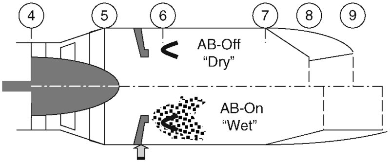
Calculate
- A4 (m2)
- A5 (m2) for M5 = 0.5
- fAB
- Ag (m2) “dry”
- Ag (m2) “wet”
- A9/A8 “dry” for p9 = p0 = 100 kPa
- A9/A8 “wet” for p9 = p0 = 100 kPa
- nozzle gross thrust (kN) “dry”
- nozzle gross thrust (kN) “wet”
- 11.8 A turbojet engine has the following design-point parameters:
Calculate
- fuel-to-air ratio f
-
turbine total temperature ratio τt

For the following off-design operation

Assume a calorically perfect gas with γ = 1.4 and cp = 1004 kJ/kg · K constant throughout the engine, and calculate
- πc–off-design
- the ratio of corrected shaft speeds Nc2, O–D/Nc2, D
- the corrected mass flow rate at off-design (kg/s)
- the axial Mach number at the engine face, Mz2, atoff-design
- thrust-specific fuel consumption at design and off-design in mg/s/N
- 11.9 A separate-flow turbofan engine has a dual spool configuration, as shown. Fan and core nozzles are convergent and choked.

The design parameters for this engine are:
- M0 = 0, p0 = 101.33 kPa, T0 = 15.2°C
- πd = 0.98
- πf = 1.8, ef = 0.90
- α = 5.0
- πcH = 14, ecH = 0.90
- Tt4 = 1600°C, QR = 42, 800 kJ/kg, ηb = 0.99, πb = 0.95
- etH = 0.85, ηmH = 0.995
- etL = 0.89, ηmL = 0.995
- πn = πnf = 0.98, p8 = p18 = p0
- γc = 1.4, cpc = 1004 J/kg · K
- γt = 1.33, cpt = 1146 J/kg · K
- M4 = M4.5 = M9 = M19 = 1.0
An off-design operating condition is described by
- M0 = 0.90, p0 = 20 kPa, T0 = −20°C
- Tt4 = 1300°C
Assuming all component efficiencies remain constant, calculate
- fan pressure ratio πf
- high-pressure compressor pressure ratio πcH
- the bypass ratio α
- 11.10 A turbojet engine has the following design parameters (which is at takeoff):


This engine powers an aircraft that cruises at M0 = 0.80 at an altitude where T0 = −35°C, p0 = 20 kPa. The turbine entry temperature at cruise is Tt4 = 1500°C. Assume that the engine has the same component efficiencies at cruise and takeoff, and the nozzle is perfectly expanded at cruise, as well.
Calculate
- the exhaust velocity V9 (in m/s) at the design point, i.e., at takeoff
- the thermal efficiency ηth at the design point
- thrust-specific fuel consumption at the design point
- the compressor pressure ratio at cruise
- the exhaust velocity V9 (in m/s) at cruise
- the thermal efficiency ηth at cruise
- the propulsive efficiency ηp at cruise
- the thrust-specific fuel consumption at cruise
- 11.11 In a gas generator, the compressor and burner performance maps are shown. The turbine adiabatic efficiency is assumed nearly constant at ηt = 0.85. The nominal operating line on the compressor performance map represents the Tt4/Tt2 = 7.0 throttle line.

The design corrected shaft speed is Nc2 = 10, 000 rpm and the compressor pressure ratio at design is πc, D = 13.5 (note that the corrected mass flow rate at the compressor face is 89 kg/sat design).
Assuming

Calculate and graph the gas generator pumping characteristics, as percent corrected shaft speed Nc2 (% design).
- 11.12 The gas generator in Problem 11.11 is to be matched to a variable-throat area convergent nozzle, as shown.
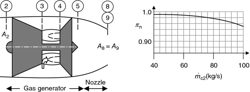
The nozzle performance map is also shown here as a graph of πn versus the corrected mass flow rate (at the engine face). First, by matching the mass flow rate at station 8 (or 9) to that of 2, show that the corrected mass flow rates at 8 (or 9) and 2 are related to pumping characteristics according to

Assuming the nozzle throat remains choked, i.e., M8 = 1.0, graph A8 variation (or percentage A8/A8, D variation) as a function of the percent-design corrected shaft speed Nc2 (% design).
- 11.13 A separate-flow turbofan engine has the following design-point parameters:
- M0 = 0, p0 = 0.1 MPa, T0 = 15°C
- πd = 0.98
- πf = 1.65, ef = 0.90
- α = 7.0
- πcH = 20, ecH = 0.90
- Tt4 = 1650°C, QR = 42, 800 kJ/kg, ηb = 0.99, πb = 0.95
- etH = 0.85, ηmH = 0.995
- etL = 0.89, ηmL = 0.995
- πn = πnf = 0.98, p8 = p18 = p0
- γc = 1.4, cpc = 1004 J/kg · K
- γt = 1.33, cpt = 1146 J/kg · K
- M4 = M4.5 = M8 = M18 = 1.0
The off-design operation of this engine is represented by a cruise altitude flight such as

Assuming all other efficiencies and gas properties remaining constant, calculate the following parameters at off-design condition:
- fan pressure ratio πf
- high-pressure compressor pressure ratio πcH
- bypass ratio α
- 11.14 A turbojet engine has the following design-point parameters:
- M0 = 0, p0 = 0.1 MPa, T0 = 15°C
- πd = 0.98
- πc = 15, ec = 0.90
- QR = 42, 800 kJ/kg, πb = 0.97, ηb = 0.98, Tt4 = 1485°C
- et = 0.80, ηm = 0.995

- Nc2 (rpm) = 6, 000
- Mz2 = 0.6
- πn = 0.97, p9/p0 = 1.0
The off-design flight condition is described by

Assuming all other component efficiencies (except πd that is specified) remain the same (as design) at off-design and gas properties are γc = γt=1.4 and cpc = cpt=1004 J/kg · K, calculate
- πc-O–D
 (in kg/s)
- Nc2, O–D (in rpm)
- Mz2, O–D
- 11.15 An afterburning turbojet engine’s design-point parameters are
- M0 = 0, p0 = 101.33 kPa, T0 = 288.2 K, γc = 1.4, cpc = 1004 J/kg · K
- πd = 0.95
- πc = 18, ec = 0.90

- Nc2 = 7120 rpm
- Mz2 = 0.5
- QR = 42, 800 kJ/kg, πb = 0.98, ηb = 0.97, Tt4 = 1773 K
- γt = 1.33, cpt = 1156 J/kg · K
- et = 0.80, ηm = 0.995
- QR, AB = 42, 800 kJ/kg, πAB = 0.95, ηAB = 0.98, Tt7 = 2250 K
- γAB = 1.3, cpc = 1243 J/kg · K
- πn = 0.90, p9/p0 = 1.0
The off-design conditions correspond to supersonic flight at high altitude

Calculate
- compressor pressure ratio at off-design
- the corrected and physical mass flow rates at the compressor face at off-design in kg/s
- the fuel-to-air ratio at off-design
- the exhaust speed at off-design in m/s
- thrust specific fuel consumption in mg/s/N at on- and off-design
- 11.16 A turbojet engine has a design corrected mass flow rate of
 at the standard sea level static condition. The design axial Mach number at the engine face is Mz2 = 0.5. Calculate the engine face flow area, A2, in m2 (γ = 1.4, R = 287 J/kg · K, pSL = 101 kPa and TSL = 288 K).
 - 11.17 A turbojet engine has choked nozzles both in turbine as well as exhaust. Its design point is at the standard sea level static condition (pSL = 101 kN and TSL = 288 K) and the design calculations yield a turbine expansion parameter of τt = 0.70. Assuming design parameters are: Tt4-D = 1950 K, f = 0.023, ηm = 0.993 and ec = 0.9, estimate:
- compressor pressure ratio at design, πc-D
- compressor pressure ratio at off-design, πc-OD
Where the off-design condition is described by: M0 = 2.0, p0 = 25 kPa, T0 = 223 K, Tt4, OD = 1650 K.
Assume the same component efficiencies and fuel-to-air ratio in on- and off-design and constant gas properties, i.e., assume γc = γt = 1.4, cpc = cpt = 1004 J/kg · K.
- 11.18 In a compressor performance map, the design corrected mass flow rate is
 and the design compressor pressure ratio is πc − D = 30. The mass flow rate at stall drops to 238.1 kg/s and the corresponding compressor pressure ratio at stall rises to 31.5. Calculate
- the compressor stall margin, SM (%)
- estimate the drop in axial Mach number between the design point and stall, i.e., Mz2-D – Mz2-Stall, assuming Mz2-D = 0.5.

- 11.19 A high bypass ratio separate-flow turbofan engine with convergent nozzles has the following design point parameters (at takeoff, standard sea-level conditions):

The off-design point is the cruise condition described by:

Calculate C1, C2 and C3 parameters at the design point. Then use Equation 11.67 to solve, i.e., to iterate for, τcH-OD. Then, calculate τf-OD and αOD. Use polytropic efficiencies to get πf and πcH at off-design.
For a turbofan engine, the corrected mass flow rate at the engine face relates to off-design condition according to:
where πc is the overall pressure ratio, namely πf.πcH.
Then use the corrected mass flow rate at the engine face to calculate the physical mass flow rate at cruise.
- 11.20 Cruise flight condition is: M0 = 0.85, altitude is 12 km (U.S. standard atmosphere), with
 . Assuming that the inlet total pressure recovery at cruise is 0.995, calculate
- corrected mass flow rate,
 , in kg/s
 - captured stream area, A0, in m2
- physical mass flow rate of air,
 , in kg/s
 - inlet throat area (assume
 ), neglecting the total pressure loss from highlight to throat
 - ram drag in kN
- corrected mass flow rate,