4.5 The Turboprop Engine

4.5.1 Introduction

To construct a turboprop engine, we start with a gas generator.

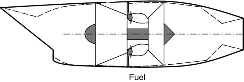
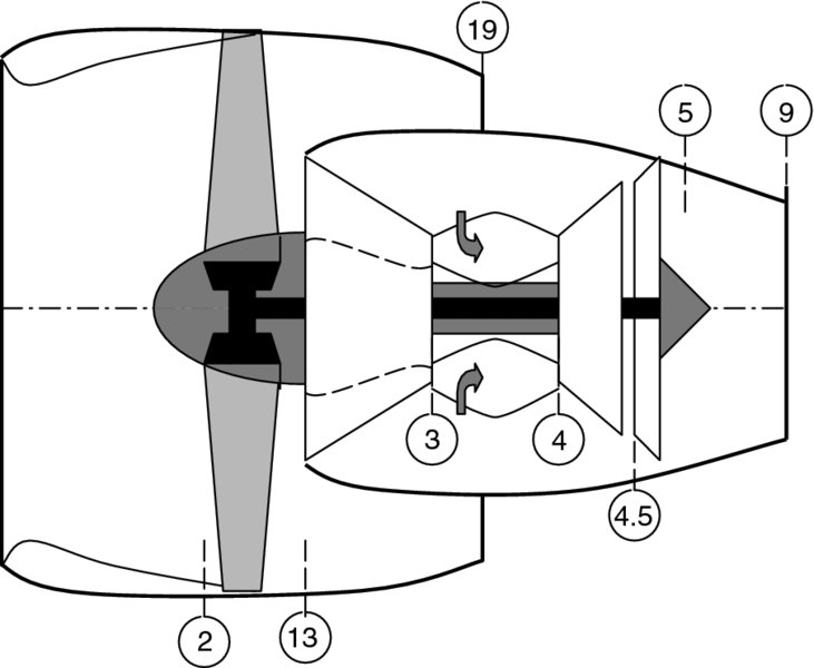
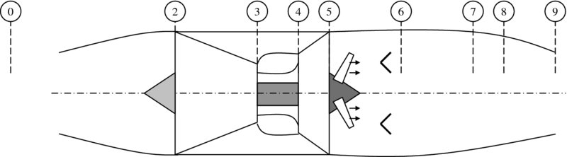
The turbine in the gas generator provides the shaft power to the compressor. However, we recognize that the gas in station 5 is still highly energetic (i.e., high p_t and T_t) and capable of producing shaft power, similar to a turbofan engine. Once this shaft power is produced in a follow-on turbine stage that is called “power” or “free” turbine, we can supply the shaft power to a propeller. A schematic drawing of this arrangement is shown in Figure 4.51.

The attractiveness of a turbopropeller engine as compared with a turbofan engine lies in its ability to offer a very large bypass ratio, which may be between 30 and 100. The large bypass ratio, by necessity, will then cut back on the exhaust velocities of the propulsor, thereby attaining higher propulsive efficiencies for the engine. The high propulsive efficiency, however, comes at a price. The limitation on the tip Mach number of a rotating propeller, say to less than 1.3, leads to a cruise Mach number in the 0.7–0.8 range for advanced turboprops and to 0.4–0.6 for conventional propellers. We do not have this limitation on cruise Mach number in a turbofan engine. Also, the large diameter of the propeller often requires a reduction gearbox that adds to the engine weight and system complexity with its attendant reliability and maintainability issues.

Before we start our discussion of turboprop engines, it is appropriate to present basic concepts in propeller theory with applications to performance, sizing and selection.

4.5.2 Propeller Theory

Propellers are means of converting mechanical shaft (torque) power efficiently into forward/reverse thrust power in a vehicle. Although our application is in aircraft in this book, the same function and principles hold in a marine vehicle, that is, surface ships and submarines. There are two classical approaches to propeller theory:

1. Momentum or actuator disk theory
2. Blade element theory.

The pioneers of the momentum or actuator disk theory are Rankine (1865) and Froude (1889). The momentum theory replaces the propeller by a circular actuator disk that creates a jump in swirl, and thus angular momentum, across the disk, as well as a jump in static pressure. The product of the static pressure jump and the propeller disk area is then interpreted as the propeller thrust. The jump in the angular momentum is then related to the shaft (or torque) power that is delivered to and absorbed by the propeller. Individual blades lose their meaning in the actuator disk theory since they are smeared into an axisymmetric disk. The shaft power is not delivered to individual propeller blades either, since there are no individual blades, rather a uniform disk. Therefore, the shaft power, too, is smeared into a parameter that is described by power disk loading, which is the shaft power per unit disk area. In the absence of discrete propeller blades, the resulting swirling flow downstream of the actuator disk is uniformly swirling in the azimuthal direction. The flow process is further assumed to be completely steady and the fluid is treated as incompressible and inviscid. With these limitations, elegant ideal solutions are obtained that represent the ideal or the upper limit of the performance of a propeller.

4.5.2.1 Momentum Theory

A definition sketch is shown in Figure 4.52, which depicts a captured stream tube with free stream conditions at its entrance, an actuator disk, of area A_p corresponding to the propeller disk area and a uniformly swirling flow downstream of the actuator disk that extends to far downstream conditions.

As indicated by the definition sketch, V₀ is the forward speed of the propeller; p₀ and ρ₀ are the ambient pressure and density, which are essentially altitude dependent flight parameters. The axial velocity at the disk is V_p, which is continuous across the disk (to satisfy the continuity equation across the disk for incompressible fluid) and different from the forward speed of the propeller. We will show that the axial velocity at the propeller disk is the average of far upstream and downstream speeds, V₀ and V₁ respectively. The static pressure undergoes a jump across the disk. The disk area is A_p. Upstream flow has no swirl whereas downstream flow is uniformly swirling with V_θp′, as shown. Far downstream of the propeller disk flow is uniform and recovers the ambient static pressure, p₀ and attains an axial velocity of V₁ and swirl velocity of V_θ1. Due to small velocity variations from station 0 to 1, the fluid is considered to be incompressible where ρ = ρ₀.

Typically, there are six known parameters, namely:

• flight condition, V₀, p₀ and ρ₀
• propeller diameter, therefore disk area, A_p
• shaft power delivered to (and absorbed by) the propeller, ℘_p
• propeller shaft angular speed, ω.

There are eight unknowns, A₀, A₁, V_p, V_θp′, V₁, V_θ1, p_p and p_p′.

We apply conservation principles of mass, linear and angular momentum and energy to solve this problem. Continuity demands that

(4.198)

The Bernoulli equation, that is, the integral of linear momentum in an incompressible, inviscid and steady flow, applies along a stream surface upstream of the disk, namely

(4.199)

Note that we have neglected the radial velocity contribution at the propeller face. The Bernoulli equation downstream of the disk, again with negligible radial velocity contribution, yields:

(4.200)

The axial momentum balance between stations 0 and 1 is equal to the net external forces in the z-direction acting on the fluid, according to Newton’s second law of motion, that is,

(4.201)

Note that the jump in static pressure across the disk results in propeller thrust that is in the –z direction and its reaction that acts on the fluid is in the +z direction. Furthermore, an approximation is made in writing Equation 4.201 that assumes the streamwise integrals of static pressure on the captured stream tube upstream and downstream of the propeller are small compared to the propeller thrust term. Von Mises (1959) offers more elaborate discussion on the assumptions that lead to Equation 4.201 for propeller thrust in momentum theory.

The power absorbed by the propeller appears as the thrust power of the propeller plus the change in the rate of kinetic energy between stations 0 and 1, namely

(4.202)

where

(4.203)

Finally, the law of conservation of angular momentum applied to flow immediately downstream of the propeller disk and far downstream station, yields two equations for propeller torque, which produces shaft power when combined with propeller shaft angular speed, ω, according to:

(4.204a)

(4.204b)

The two swirl terms, and , on the RHS of Aquations 4.204a and 4.204b, are the (torque-based) mean swirl far downstream and immediately downstream of the propeller, respectively. Now, based on the conservation principles in fluids, we have written eight coupled nonlinear equations that involve the eight unknowns. Following Rankine, two additional approximations to the flow may be introduced that simplify our task significantly and lead to an elegant solution. The first approximation is to neglect the change in the swirl kinetic energy in Bernoulli equation (4.200) and the second approximation drops the swirl kinetic energy term in power balance equation (4.202) in favor of the propeller thrust power and the axial kinetic energy change. The approximate equations can be summarized:

(4.205)

(4.206)

(4.207)

If we subtract the two Bernoulli equations (4.199 and 4.205), we get:

(4.208)

Now, substitute for F_prop/A_p in Equation 4.208 from Equation 4.207 to get:

(4.209)

Within these approximations, the flow speed at the propeller plane is the average of the flight speed and far downstream of the propeller.

We substitute for the propeller thrust in the energy equation (4.206) from Equation 4.207 to get:

(4.210)

If we substitute for V_p from Equation 4.209, the above equation would only contain a single unknown, namely, V₁. The resulting equation is a cubic in V₁/V₀:

(4.211)

The left-hand side of Equation 4.211 is nondimensional power with all terms known, which may be referred to as the propeller power loading, C_P. The RHS of Equation 4.211 is a cubic in velocity ratio, V₁/V₀. Note that the shaft power vanishes when the velocity ratio V₁/V₀ approaches 1.

Finally, on the discussion of efficiency, we have propeller efficiency that is defined as the fraction of propeller shaft power that is converted to the propeller thrust power, namely

(4.212)

By applying propulsive efficiency definition to the stream tube upstream and downstream of the propeller, we get:

(4.213)

We note that the propeller and propulsive efficiencies in Equations 4.212 and 4.213 are related to each other and indeed propulsive efficiency is the ideal limit of the propeller efficiency, since

(4.214)

where

(4.215)

In Equation 4.215, η_L, is the efficiency of propeller in converting its shaft power into stream kinetic power. Since propulsive efficiency (Equation 4.213) is the maximum, or the limit, efficiency of a propeller, it is often times calculated and reported as the “ideal” propeller efficiency in literature. Further discussion on propeller and propulsive efficiencies may be found in Oates (1988) and Lan-Roskam (1997).

Let us solve two propeller problems using the momentum theory.

4.5.2.2 Blade Element Theory

Another approach proposed to study the aerodynamic design and performance of propellers is blade element theory. The foundation of this theory is found in the classical airfoil and wing theory. A propeller is a spinning (twisted) wing, with angular speed ω = 2πn, with its span-wise elements in solid-body rotation. The rotational speed increases linearly with distance from the axis of rotation, r, hence the need for twist. Therefore, by virtue of rotation, the blade sections are subjected to relative flow magnitude and angle, that is, as seen by the blade element. A propeller blade is composed of airfoil sections along its span that see the relative flow and create local aerodynamic forces and torques. The aerodynamic performance of the sections depends on the local relative flow speed, airfoil profile, and angle of attack (as seen by the section) and Reynolds number based on chord and relative speed. Figure 4.53 is a definition sketch that shows a propeller and its sectional velocity vectors and angles with elemental aerodynamic force components.

The relative flow, or the relative wind V_R, is created as the vector sum of flight and the blade rotational speed at any element along the span. The relative flow angle is , which is also called the helix angle. The aerodynamic lift on the blade element is proportional to the local effective angle of attack, which is composed of: (i) the geometric angle of attack; (ii) the angle-of-zero lift (due to airfoil camber); and (iii) the induced angle of attack (due to the trailing vortices in the propeller wake). The basic blade element theory, however, does not account for the induced angle of attack that is caused by the 3D trailing vortices. Therefore, in the strict sense, propeller blade performance in three dimensions is constructed from the superposition of sectional 2D performance. The geometric pitch angle, β, is also shown in Figure 4.53; it is the angle that the blade element (in cambered airfoil measured from zero-lift-line) makes with respect to plane of rotation. The tangential force element multiplied by the moment arm, r, measured from the axis of rotation, creates blade element torque, dτ, as shown in Figure 4.53. The propeller parameters of interest, namely thrust and torque, are the integrals of elemental thrust and torque along the blade span. In turn, the elemental torque and thrust are related to the lift and drag components, using the pitch angle, , according to:

(4.216)

(4.217)

The lift and drag forces are proportional to lift and drag coefficients with the product of relative dynamic pressure and the local chord length as the proportionality constant, namely

(4.218)

(4.219)

The sectional propeller efficiency may be defined as:

(4.220)

A major shortcoming of blade element theory in modeling 3D propellers is in lack of 3D coupling of the propeller sections along its span, which may be partially alleviated if we incorporate the induced axial and swirl velocity components from the momentum theory. Also, the compressibility effect may cause local supersonic flow near the blade tip with the subsequent shock formation, boundary layer separation and stall. Modern supersonic tip propeller designs that use sweep are introduced in advanced turboprops (ATP) by Pratt and Whitney and GE (which is called Propfan). Further discussions on propellers, in the context of Uninhabited Aerial Systems (UAS), related to control, type and performance are presented in Chapter 5.

4.5.3 Turboprop Cycle Analysis

4.5.3.1 The New Parameters

Let us identify the new parameters that we have introduced by inserting a propeller in the gas turbine engine. We will examine the turboprop from the power distribution point of view as well as its thrust producing capabilities namely the propeller thrust contribution to the overall thrust, which includes the core thrust.

From the standpoint of power, the low-pressure turbine power is supplied to a gearbox, which somewhat diminishes it in its frictional loss mechanism in the gearing and then delivers the remaining power to the propeller. We will call the fractional delivery of shaft power through the gearbox, the gearbox efficiency η_gb, which symbolically is defined as

(4.221)

where the numerator is the power supplied to the propeller and the denominator is the shaft power provided by the power turbine to the gearbox. Also, we define the fraction of propeller shaft power that is converted in the propeller thrust power as the propeller efficiency η_prop as

(4.222)

Now, let us examine the overall thrust picture of a turboprop engine. We recognize that the propeller and the engine core both contribute to thrust production. We can express this fact as

(4.223)

The contribution of the engine core to the overall thrust, which we have called as the core thrust, takes on the familiar form of the gross thrust of the nozzle minus the ram drag of the air flow rate that enters the engine, that is,

(4.224)

The pressure thrust contribution of the nozzle, that is, the last term in Equation 4.224, for a turboprop engine is often zero due to perfectly expended exhaust, that is, p₉ = p₀. So, for all practical purposes, the engine core of a turboprop produces a thrust based solely on the momentum balance between the exhaust and the intake of the engine, namely,

(4.225)

4.5.3.2 Design Point Analysis

We require the following set of input parameters in order to estimate the performance of a turboprop engine. The following list, which sequentially proceeds from the flight condition to the nozzle exit, summarizes the input parameters per component. In this section, we will practice the powerful marching technique that we have learned so far in this book.

Station 0

The flight Mach number M₀, the ambient pressure and temperature p₀ and T₀, and air properties γ and R are needed to characterize the flight environment. We can calculate the flight total pressure and temperature p_t0 and T_t0, the speed of sound at the flight altitude a₀, and the flight speed V₀, based on the input.

Station 2

At the engine face, we need to establish the total pressure and temperature P_t2 and T_t2. From adiabatic flow assumption in the inlet, we conclude that

To account for the inlet frictional losses and its impact on the total pressure recovery of the inlet, we need to define an inlet total pressure ratio parameter π_d or adiabatic diffuser efficiency η_d. This results in establishing p_t2, similar to our earlier cycle analysis, for example,

Station 3

To continue our march through the engine, we need to know the compressor pressure ratio π_c, which again is treated as a design choice, and the compressor polytropic efficiency e_c. This allows us to calculate the compressor temperature ratio in terms of compressor pressure ratio using the polytropic exponent, that is,

Now, we have established the compressor discharge total pressure and temperature p_t3 and T_t3.

Station 4

To establish the burner exit conditions, similar to earlier analysis, we need to know the loss parameters η_b and π_b as well as the limiting temperature T_t4. The fuel type with its energy content, that we had called the heating value of the fuel, Q_R, needs to be specified. Again, we establish the fuel-to-air ratio f by energy balance across the burner and the total pressure at the exit, p_t4, by loss parameter π_b.

Station 4.5

For the upstream turbine, or the so-called the HPT, we need to know the mechanical efficiency η_mHPT, which is a power transmission efficiency, and the turbine polytropic efficiency e_tHPT, which measures the internal efficiency of the turbine. The power balance between the compressor and high-pressure turbine is

(4.226a)

(4.226b)

leads to the only unknown in the above equation, which is h_t4.5. The total pressure at station 4.5 may be linked to the turbine total temperature ratio according to

(4.227)

(4.228)

Stations 5 and 9

Since the power turbine drives a load, that is, the propeller, we need to specify the turbine expansion ratio that supports this load. In this sense, we consider the propeller as an external load to the cycle and hence as an input parameter to the turboprop analysis. It serves a purpose to put this and the following station, that is, 9, together, as both are responsible for the thrust production. Another view of stations 5 and 9 downstream of 4.5 points to the power split, decision made by the designer, between the propeller and the exhaust jet. The following T–s diagram best demonstrates this principle.

In the T–s diagram (Figure 4.54), both the actual and the ideal expansion processes are shown. We will use this diagram to define the component efficiencies as well as the power split choice. For example, we define the power turbine (i.e., LPT) adiabatic efficiency as

(4.229)

Also, we may define the nozzle adiabatic efficiency η_n as

(4.230)

We note that the above definition for the nozzle adiabatic efficiency deviates slightly from our earlier definition in that we have assumed

(4.231)

which in light of small expansions in the nozzle and hence near parallel isobars, this approximation is considered reasonable. The total ideal power available at station 4.5, per unit mass flow rate, may be written as

(4.232)

If we examine the RHS of the above equation, we note that all terms on the RHS are known. Therefore, the total ideal power is known to us a priori. Now, let us assume that the power split between the free turbine and the nozzle is, say α and 1 − α, respectively, as shown in Figure 4.55.

We can define the power split as

(4.233)

which renders the following expression for the free turbine (LPT) power in terms of a given α,

(4.234)

This expression for the power turbine (LPT) can be applied to the propeller through gearbox and propeller efficiency in order to arrive at the thrust power produced by the propeller, namely,

(4.235)

We note that the RHS of the above equation, per unit mass flow rate, is known. Now, let us examine the nozzle thrust. The kinetic energy per unit mass at the nozzle exit may be linked to

(4.236)

Therefore, the exhaust velocity is now approximated by the power split parameter α and the total ideal power available after the gas generator, that is, station 4.5, according to

(4.237)

A more accurate expression for exhaust velocity is derived based on nozzle adiabatic efficiency that is defined based on the states t5, 9 and 9i. Example 4.20 calculates the nozzle exhaust velocity using the more accurate method.

Now, the turboprop thrust per unit air mass flow rate (through the engine) can be expressed in terms of the propeller thrust of expression 4.235 and the core thrust expression 4.225 with Equation 4.237 incorporated for the exhaust velocity.

(4.238)

The fuel efficiency of a turboprop engine is often expressed in terms of the fraction of the fuel consumption in the engine to produce a unit shaft/mechanical power, according to

(4.239)

(4.240)

(4.241)

We can define the thermal efficiency of a turboprop engine as

(4.242)

The propulsive efficiency η_p may be defined as

(4.243)

where all the terms in the above efficiency definitions have been calculated in earlier steps and the overall efficiency is again the product of the thermal and propulsive efficiencies.

4.5.3.3 Optimum Power Split Between the Propeller and the Jet

For a given fuel flow rate, flight speed, compressor pressure ratio, and all internal component efficiencies, we may ask a very important question, which is “at what power split α would the total thrust be maximized?” This is a simple mathematics question. What we need first, is to express the total thrust in terms of all independent parameters, i.e., f, V₀, π_c, and so on, and then differentiate it with respect to α and set the derivative equal to zero. From that equation, obtain the solution(s) for α that satisfies the equation. We go to Equation 4.238 for an expression for the total thrust.

We express the exhaust velocity V₉ as (Equation 4.237)

We note that the bracketed term in the above equations, that is,

(4.244)

which is a constant. Also let us examine the total enthalpy at station 4.5, h_t4.5,

(4.245)

which is a constant, as well. Therefore, the expression for the total thrust of the engine (per unit mass flow rate in the engine nozzle) is essentially composed of a series of constants and the dependence on α takes on the following simplified form:

(4.246)

where C₁, C₂, and C₃ are all constants. Now, let us differentiate the above function with respect to α and set the derivative equal to zero, that is,

(4.247)

which produces a solution for the power split parameter α that maximizes the total thrust of a turboprop engine. Hence, we may call this special value of α, the “optimum” α, namely

(4.248)

Now, upon substitution for the constants C₁ and C₂ and some simplification, we get

(4.249)

This expression for the optimum power split between the propeller and the jet involves all component and transmission (of power) efficiencies, as expected. However, let us assume that all efficiencies were 100% and further assume that the exhaust nozzle was perfectly expanded, that is, p₉ = p₀. What does the above expression tell us about the optimum power split in a perfect turboprop engine? Let us proceed with the simplifications.

(4.250)

From power balance between the compressor and the high-pressure turbine, we can express the following:

(4.251)

which simplifies to

(4.252)

Substitute the above equation in the optimum power split in an ideal turboprop engine, Equation 4.250, to get

(4.253)

At takeoff condition and low-speed climb/descent (τ_r → 1), the optimum power split approaches 1, as expected. The propeller is the most efficient propulsor at low speeds, as it attains the highest propulsive efficiency. As flight Mach number increases, the power split term a becomes less than 1.

4.6 Summary

In this chapter, we learned various gas turbine engine configurations and their analysis. The performance parameters were identified to be specific thrust, specific fuel consumption, thermal, propulsive, and overall efficiencies. We had limited our approach to steady, one-dimensional flow and the “design-point” analysis. We also learned that we may analyze ramjets by setting compressor pressure ratio to one in a turbojet engine. We had essentially removed the compressor (and thus turbine) by setting its pressure ratio equal to 1. We included the effect of fluid viscosity and thermal conductivity in our cycle analysis empirically, that is, through the introduction of component efficiency. The knowledge of component efficiency at different operating conditions is critical to their design and optimization. We always treated that knowledge, that is, the component efficiency, as a “given” in our analysis. In reality, engine manufacturers, research laboratories, and universities continually measure component performance and sometimes report them in open literature. However, commercial engine manufacturers treat most competition-sensitive data as proprietary. Propeller theory is treated as a part of turboprop cycle analysis.

In the following six chapters, we will take on the propulsion system of Uninhabited Aerial Vehicles (UAV) and then follow this with engine component analysis. The nonrotating components, that is, inlets and nozzles, are treated in a single chapter (Chapter 6). An introductory study of combustion and the gas turbine burner and afterburner configurations follows in Chapter 7. The rotating components, that is, compressors and turbines, are treated in the turbomachinery Chapters 8–10. Finally, we allow components to be “matched” and integrated in a real engine where we explore its off-design analysis in Chapter 11: Component Matching and Engine Off-design Analysis.

References 1–11 provide for complementary reading on aircraft propulsion and are recommended to the reader.

References

1. Archer, R.D. and Saarlas, M., An Introduction of Aerospace Propulsion, Prentice Hall, New York, 1998.
2. Cumpsty, N., Jet Propulsion: A Simple Guide to the Aerodynamic and Thermodynamic Design and Performance of Jet Engines, 2nd edition, Cambridge University Press, Cambridge, UK, 2003.
3. Flack, R.D. and Rycroft, M.J., Fundamentals of Jet Propulsion with Applications, Cambridge University Press, Cambridge, UK, 2005.
4. Heiser, W.H., Pratt, D.T., Daley, D.H., and Mehta, U.B., Hypersonic Airbreathing Propulsion, AIAA, Washington, DC, 1993.
5. Hesse, W.J. and Mumford, N.V.S., Jet Propulsion for Aerospace Applications, 2nd edition, Pittman Publishing Corporation, New York, 1964.
6. Hill, P.G. and Peterson, C.R., Mechanics and Thermodynamics of Propulsion, 2nd edition, Addison-Wesley, Reading, Massachusetts, 1992.
7. Kerrebrock, J.L., Aircraft Engines and Gas Turbines, 2nd edition, MIT Press, Cambridge, Mass, 1992.
8. Mattingly, J.D., Elements of Gas Turbine Propulsion, McGraw-Hill, New York, 1996.
9. Mattingly, J.D., Heiser, W.H., and Pratt, D.T., Aircraft Engine Design, 2nd edition, AIAA, Washington, DC, 2002.
10. Oates, G.C., Aerothermodynamics of Gas Turbine and Rocket Propulsion, AIAA, Washington, DC, 1988.
11. Shepherd, D.G., Aerospace Propulsion, American Elsevier Publication, New York, 1972.
12. Asbury, S.C. and Yetter, J.A., Static Performance of Six Innovative Thrust Reverser Concepts for Subsonic Transport Applications, NASA/ TM 2000-210300, National Aeronautics and Space Administration, Langley Research Center, Hampton, VA, July 2000.
13. CFM, The Power of Flight. http://www.cfmaeroengines.com/; last accessed 24 November 2013.
14. Duong, L., McCune, M., and Dobek, L., Method of Making Integral Sun Gear Coupling, United States Patent 2009/0293278, 3 December 2009.
15. Guynn, M.D. Berton, J.J. Fisher, K.L. et al., Engine Concept Study for an Advanced Single-Aisle Transport”, NASA TM 2009-215784, National Aeronautics and Space Administration, Langley Research Center, Hampton, VA, August 2009.
16. Halliwell, I., AIAA-IGTI Undergraduate Team Engine Design Competition Request for Proposal, 2010–2011; www.aiaa.org; last accessed 24 November 2013.
17. Kurzke, J., A design and off-design performance program for gas turbines, GasTurb, 2013. http://www.gasturb.de; last accessed 24 November 2013.
18. Lan, C.T. and Roskam, J., Airplane Aerodynamics and Performance, DAR Corporation, Lawrence, KA, 2008.
19. Pratt & Whitney, Geared Turbo Fan. http://www.pw.utc.com/PurePowerPW1000G_Engine; last accessed 24 November 2013.
20. Von Mises, R., Theory of Flight, Dover Publications, New York, 1959.

Problems

• 4.1 An aircraft is flying at an altitude where the ambient static pressure is p₀ = 25 kPa and the flight Mach number is M₀ = 2.5. The total pressure at the engine face is measured to be p_t2 = 341.7 kPa. Assuming the inlet flow is adiabatic and γ = 1.4, calculate
  1. the inlet total pressure recovery π_d
  2. the inlet adiabatic efficiency η_d
  3. the nondimensional entropy rise caused by the inlet Δs_d/R
• 4.2 A multistage axial-flow compressor has a mass flow rate of 100 kg/s and a total pressure ratio of 25. The compressor polytropic efficiency is e_c = 0.90. The inlet flow condition to the compressor is described by T_t2 = −35°C and p_t2 = 30 kPa. Assuming the flow in the compressor is adiabatic, and constant gas properties throughout the compressor are assumed, i.e., γ = 1.4 and c_p = 1004 J/kg · K, calculate
  1. compressor exit total temperature T_t3, in K
  2. compressor adiabatic efficiency η_c
  3. compressor shaft power ℘_c in MW
• 4.3 A gas turbine combustor has inlet condition T_t3 = 900 K, p_t3 = 3.2 Mpa, air mass flow rate of 100 kg/s, γ₃ = 1.4, c_p3 = 1004 J/kg · K.

  A hydrocarbon fuel with ideal heating value Q_R = 42, 800 kJ/Kg is injected in the combustor at a rate of 2 kg/s. The burner efficiency is η_b = 0.99 and the total pressure at the combustor exit is 97% of the inlet total pressure, i.e., combustion causes a 3% loss in total pressure. The gas properties at the combustor exit are γ₄ = 1 .33 and c_p4 = 1, 156 J/kg · K. Calculate

  1. fuel-to-air ratio f
  2. combustor exit temperature T_t4 in K and p_t4 in MPa
• 4.4 An uncooled gas turbine has its inlet condition the same as the exit condition of the combustor described in Problem 4.3. The turbine adiabatic efficiency is 85%. The turbine produces a shaft power to drive the compressor and other accessories at ℘_t = 60 MW. Assuming that the gas properties in the turbine are the same as the burner exit in Problem 4.3, calculate
  1. turbine exit total temperature T_t5 in K
  2. turbine polytropic efficiency e_t
  3. turbine exit total pressure p_t5 in kPa
  4. turbine shaft power ℘_t based on turbine expansion ΔT_t
• 4.5 In a turbine nozzle blade row, hot gas mass flow rate is 100 kg/s and h_tg = 1900 kJ/kg. The nozzle blades are internally cooled with a coolant mass flow rate of 1.2 kg/s and h_tc = 904 kJ/kg as the coolant is ejected through nozzle blades trailing edge. The coolant mixes with the hot gas and causes a reduction in the mixed-out enthalpy of the gas. Calculate the mixed-out total enthalpy after the nozzle. Also for the c_{p, mixed-out} = 1594 J/kg · K, calculate the mixed out total temperature.
• 4.6 Consider the internally cooled turbine nozzle blade row of Problem 4.5. The hot gas total pressure at the entrance of the nozzle blade is p_t4 = 2.2 MPa, c_pg = 1156 J/kg · K, and γ_g = 1.33. The mixed-out total pressure at the exit of the nozzle has suffered 5% loss due to both mixing and frictional losses in the blade row boundary layers. Calculate the entropy change Δs/R across the turbine nozzle blade row.
• 4.7 A convergent–divergent nozzle with a pressure ratio, NPR = 12. The gas properties are γ = 1.33 and c_p = 1156 J/kg · K and remain constant in the nozzle. The nozzle adiabatic efficiency is η_n = 0.94. Calculate
  1. nozzle total pressure ratio π_n
  2. nozzle area ratio A₉/A₈ for a perfectly expanded nozzle
  3. nozzle exit Mach number M₉ (perfectly expanded)
• 4.8 Calculate the propulsive efficiency of a turbojet engine under the following two flight conditions that represent takeoff and cruise, namely
  1. V₀ = 100 m/s and V₉ = 2000 m/s
  2. V₀ = 750 m/s and V₉ = 2000 m/s
• 4.9 A ramjet is in supersonic flight, as shown. The inlet pressure recovery is π_d = 0.90. The combustor burns hydrogen with Q_R = 117, 400 kJ/kg at a combustion efficiency of η_b = 0.95. The nozzle expands the gas perfectly, but suffers from a total pressure loss of π_n = 0.92. Calculate
  1. fuel-to-air ratio f
  2. nozzle exit Mach number M₉
  3. specific (net) thrust (in N/kg/s)
  4. η_th, engine thermal efficiency
  5. η_p, engine propulsive efficiency

  

• 4.10 A ramjet takes in 100 kg/s of air at a Mach 2 flight condition at an altitude where p₀ = 10 kPa and T₀ = −25°C. The engine throttle setting allows 3 kg/s of fuel flow rate in the combustor where a hydrocarbon fuel of 42, 800 kJ/kg heating value is burned. The ramjet component efficiencies are all listed on the engine cross section. Note that the exhaust nozzle is not perfectly expanded. We intend to establish some performance parameters for this engine as well as some flow areas (i.e., physical sizes) of this engine.

  

  Assuming the gas properties are split into a cold section and a hot section (perfect gas properties), namely, γ_c = 1.4 and c_pc = 1.004 kJ/kg · K and γ_h = 1.33 and c_ph = 1.156 kJ/kg · K (subscript “c” stands for “cold” and “h” for “hot”), calculate

  1. ram drag in kN
  2. the inlet capture area A₀ in m²
  3. p_t4 in kPa
  4. T_t4 in K
  5. p_t9 in kPa
  6. exit Mach number M₉
  7. exhaust velocity V₉
  8. nozzle exit area A₉ in m²
  9. gross thrust in kN
  10. thermal efficiency ^*η_th
  11. propulsive efficiency ^*η_p
• 4.11 A mixed-exhaust turbofan engine is described by the following design and limit parameters:

  Flight:	M0 = 2.2, p0 = 10 kPa, T0 = −50°C, R = 287 J/kg · K, γ = 1.4
  Inlet mass flow rate and total pressure recovery:	(1 + α) = 25 kg/s, πd = 0.85
  Compressor, fan:	πc = 15, ec = 0.90, πf = 1.5, ef = 0.90
  Burner:	πb = 0.95, ηb = 0.98, QR = 42, 800 kJ/kg, Tt4 = 1400°C
  Turbine:	et = 0.92, ηm = 0.95, M5 = 0.5
  Mixer:	πM, f = 0.98
  Afterburner:	None
  Nozzle:	πn = 0.90, p9/p0 = 1.0

  

  Calculate

  1. ram drag D_R in kN
  2. p_t2 in kPa, T_t2 in K
  3. p_t3 in kPa, T_t3 in K
  4. p_t13 in kPa, T_t13 in K
  5. p_t4 in kPa, T_t5 in K
  6. fuel-to-air ratio f
  7. bypass ratio α, in kg/s, and in kg/s
  8. T_t6M in K
  9. p_t9 in kPa, T_t9 in K
  10. M₉, V₉ in m/s
  11. gross thrust F_g in kN
  12. thrust-specific fuel consumption in mg/s/N

  You may assume constant gas properties γ and R throughout the engine.

  We may also assume that the flow in the fan duct, i.e., between stations 13 and 15, is frictionless and adiabatic.

• 4.12 In the afterburning turbojet engine shown, assume constant gas properties and ideal components to calculate
  1. ram drag
  2. compressor shaft power ℘_c
  3. fuel-to-air ratio in the primary burner
  4. τ_λ, the limit enthalpy parameter in the gas generator
  5. turbine expansion parameter τ_t
  6. turbine shaft power ℘_t
  7. τ_λAB, the afterburner limit enthalpy parameter
  8. fuel-to-air ratio in the afterburner
  9. nozzle gross thrust
  10. engine thrust specific fuel consumption
  11. engine net uninstalled thrust
  12. engine thermal efficiency
  13. engine propulsive efficiency

  

• 4.13 An ideal separate-exhaust turbofan engine has the following design parameters:
  

  Assuming the gas is calorically perfect with γ = 1.4 and c_p = 1.004 kJ/kg · K, calculate

  1. compressor exit pressure p_t3 in kPa
  2. fan exit temperature T_t13 in K
  3. fuel-to-air ratio f
  4. turbine exit temperature T_t5 in K
  5. fan nozzle exit Mach number M₁₉
  6. core nozzle exit Mach number M₉
  7. core nozzle exit velocity V₉ in m/s
  8. The ratio of fan-to-core thrust F_fan/F_core
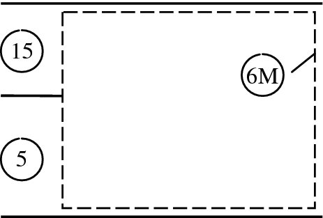
• 4.14 In a mixed-exhaust turbofan engine, we have calculated the parameters shown on the engine diagram.

  

  Assuming constant gas properties between the two streams and constant total pressure between the hot and cold gas streams, calculate

  1. the mixer exit total temperature T_t6M
  2. M₉
  3. V₉
  4. 
• 4.15 In an afterburning gas turbine engine, the exhaust nozzle is equipped with a variable area throat. Calculate percentage increase in nozzle throat area needed to accommodate the engine flow in the afterburning mode. With the afterburner on, the nozzle mass flow rate increases by 3%, the nozzle total temperature doubles, i.e. (T_t8)_AB-ON/(T_t8)_AB-OFF = 2, and the total pressure at the nozzle entrance is reduced by 20%. You may assume the gas properties γ and R remain constant and the nozzle throat remains choked.
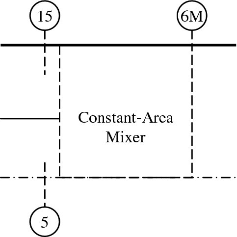
• 4.16 For the constant-area ideal mixer shown, assuming constant gas properties, calculate
  1. p₅ (kPa)
  2. p₁₅ (kPa)
  3. p_6M (kPa)

  

• 4.17 A turbojet engine has the following parameters at the on-design operating point:
  

  Calculate

  1. p_t3 and τ_c
  2. fuel-to-air ratio f and p_t4

  3. τ_t

  Now for the following off-design condition:

  
  1. compressor pressure ratio at the off-design operation
• 4.18 A turbojet engine has the following design point parameters:
  

  Calculate

  1. fuel-to-air ratio f

  2. turbine total temperature ratio τ_t

     For the following off-design operation:

     

     Assume γ = 1.4, c_p = 1004 kJ/kg · K and calculate

  3. π_c-Off-Design if τ_t-Design = τ_t-Off-Design

  

• 4.19 An ideal turbojet engine has the following design and limit parameters, namely,
  • M₀ = 2.0, altitude 37 kft
  • compressor pressure ratio π_c
  • maximum enthalpy ratio τ_λ = 7.0
  • fuel type is hydrocarbon with Q_R = 42, 800 kJ/kg
  • assume constant gas properties c_p = 1.004 kJ/kg · K and γ = 1.4.

  For a range of compressor pressure ratios, namely, 1 ≤ π_c ≤ 40, calculate and graph (using MATLAB or a spreadsheet)

  1. engine (nondimensional) specific thrust F_n/()
  2. thrust specific fuel consumption in mg/s/N
  3. in order to assess the effect of gas property variations with temperature on the engine performance parameters, repeat parts (a) and (b) for the following gas properties:
     
  4. To assess the effect of inlet total pressure recovery on the engine performance, calculate and graph the engine specific thrust and fuel consumption for a single compressor pressure ratio of π_c = 20, but vary π_d from 0.50 to 1.0. Use gas properties of part (c)
  5. Now, for the following component efficiencies
     

  

  calculate the engine performance parameters

  1. specific thrust (nondimensional)
  2. specific fuel consumption
  3. thermal efficiency
  4. propulsive efficiency
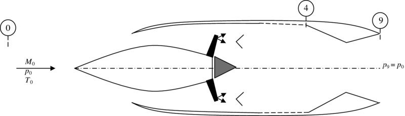
• 4.20 For an ideal ramjet, derive an expression for the flight Mach number in terms of the cycle limit enthalpy, τ_λ that will lead to an engine thrust of zero.
• 4.21 Derive an expression for an optimum Mach number that maximizes the engine-specific thrust in an ideal ramjet.
• 4.22 For an ideal ramjet with a perfectly expanded nozzle, show that the nozzle exit Mach number M₉ is equal to the flight Mach number M₀.
• 4.23 Assuming the component efficiencies in a real ramjet are
  

  For the maximum enthalpy ratio τ_λ = 8.0, the fuel heating value of 42, 000 kJ/kg and a cold and hot section gas properties

  Engine cold section:	γc = 1.40, cpc = 1.004 kJ/kg · K
  Engine hot section:	γt = 1.33, cpt = 1.156 kJ/kg · K

  calculate the optimum flight Mach number corresponding to the maximum specific thrust.

• 4.24 A ramjet uses a hydrocarbon fuel with Q_R = 42, 800 kJ/ kg flying at Mach 2 (i.e., M₀ = 2) in an atmosphere where a₀ = 300 m/s. Its exhaust is perfectly expanded and the exhaust velocity is V₉ = 1200 m/s. Assuming the inlet total pressure recovery is π_d = 0.90, the burner losses are π_b = 0.98 and η_b = 0.96, the nozzle total pressure ratio is π_n = 0.98 and λ = 1.4 and c_p = 1.004 kJ/kg · K are constant throughout the engine, calculate
  1. τ_λ
  2. fuel-to-air ratio f
  3. nondimensional-specific thrust F_n/()
  4. propulsive efficiency
  5. thermal efficiency

  

• 4.25 A large bypass ratio turbofan engine has the following design and limit parameters:
  • M₀ = 0.8, altitude = 37 kft U.S. standard atmosphere
  • π_d = 0.995
  • π_c = 40, e_c = 0.90
  • α = 6, π_f = 1.6, e_f = 0.90, π_fn = 0.98, fan nozzle is convergent
  • τ_λ = 7.0, Q_R = 42, 800 kJ/kg, π_b = 0.95, η_b = 0.98
  • e_t = 0.90, η_m = 0.975
  • π_n = 0.98, core nozzle is convergent

  Assuming the gas properties may be described by two sets of parameters, namely, cold and hot stream values, i.e.,

  Engine cold section:	γc = 1 .40, cpc = 1.004 kJ/kg · K
  Engine hot section:	γt = 1.33, cpt = 1.156 kJ/kg · K

  Calculate

  1. the ratio of compressor to fan shaft power ℘_c/℘_f
  2. fuel-to-air ratio f
  3. the ratio of fan nozzle exit velocity to core nozzle exit velocity V₁₉/V₉
  4. the ratio of two gross thrusts, F_{g, fan}/F_{g, core}
  5. the engine thermal efficiency and compare it to an ideal Carnot cycle operating between the same temperature limits
  6. the engine propulsive efficiency and compare it to the turbojet propulsive efficiency of Problem 4.19
  7. engine thrust specific fuel consumption
  8. engine (fuel)-specific impulse I_s in seconds

  

• 4.26 The flow expansion in an exhaust nozzle is shown on a T–s diagram.

  Assuming γ = 1.4, c_p = 1.004 kJ/kg · K, calculate

  1. nozzle adiabatic efficiency η_n
  2. V₉/a₀
  3. nondimensional pressure thrust, i.e.,

  

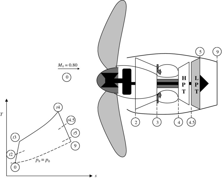
• 4.27 An advanced turboprop engine is flying at M₀ = 0.75 at 37 kft standard altitude. The component parameters are designated on the following engine drawing.

  

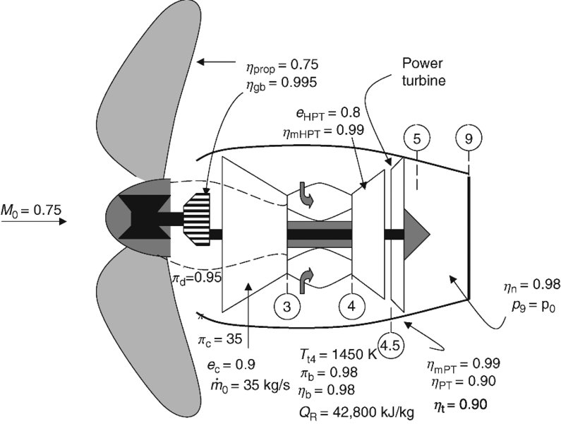
  Assuming an optimum power split α_opt that leads to a maximum engine thrust, calculate

  1. core thrust
  2. propeller thrust
  3. thrust-specific fuel consumption
  4. engine overall efficiency
• 4.28 Consider a ramjet, as shown. The diffuser total pres­sure ratio is π_d = 0 80, the burner total pressure ratio is π_b = 0 96, and the nozzle total pressure ratio is π_n = 0 90.

  Calculate

  1. fuel-to-air ratio f
  2. exit Mach number M₉
  3. nondimensional-specific thrust, i.e.,

  

• 4.29 A turbojet engine flies at V₀ = 250 m/s with an exhaust velocity of V₉ = 750 m/s. The fuel-to-air ratio is 2% and the actual fuel heating value is Q_{R, actual} = 40, 800 kJ/kg. Estimate the engine propulsive and thermal efficiencies, η_p and η_th.

  Assume the nozzle is perfectly expanded.

  

• 4.30 Consider a turboprop engine with the following parameters (note that the nozzle is convergent):
  • = 20 kg/s
  • V₀ = 220 m/s
  • η_prop = 0.80
  • η_gb = 0.995
  • η_mLPT = 0.99

  

  Calculate

  1. propeller thrust F_prop in kN
  2. nozzle gross thrust F_{g, core} in kN
  3. M₉
  4. core net thrust F_{n, core} in kN, assume f = 0.02
  5. nozzle adiabatic efficiency η_n
  6. power turbine adiabatic efficiency η_PT

  Assume γ = 1.4, c_p = 1.004 kJ/kg · K.

• 4.31 A constant-area mixer operates with the inlet conditions as shown.

  

  Assuming the hot stream has a total temperature of

  

  Calculate

  1. the ratio of mass flow rates
  2. A_6M/A₅
  3. from impulse
  4. T_t6M/T_t5
• 4.32 Consider a turboprop engine with the power turbine driving a propeller, as shown. The power turbine inlet and exit total temperatures are T_t4.5 = 783 K and T_t5 = 523 K. The mass flow rate through the turbine is 25 kg/s. Assuming c_p = 1, 100 J/kg · K.

  Calculate

  1. the power produced by the turbine
  2. the power delivered to the propeller
  3. the propeller thrust F_prop

  

• 4.33 Let us study a family of turbojet engines, all with the same component parameters except the burner, as shown on the T–s diagram. The family of turbojets are at the standard sea-level condition and stationary, i.e., M₀ = 0. The fixed engine parameters are
  • π_d = 0.995
  • π_c = 20, e_c = 0.90, γ_c = 1.4, c_pc = 1, 004 J/kg · K
  • π_b = 0.95, η_b = 0.98, Q_R = 42, 800 kJ/kg
  • η_m = 0.99, e_t = 0.85, γ_t = 1.33, c_pt = 1, 146 J/kg · K
  • π_n = 0.98
  • p₉/p₀ = 1

  

  The burner exit temperature ranges from T_t4 = 1600 K to 2400 K. Calculate and graph

  1. nondimensional-specific gross thrust versus T_t4
  2. specific impulse I_s (based on fuel flow rate) in seconds versus T_t4
  3. T₉/T₀ versus T_t4
  4. thermal efficiency, η_th versus T_t4
• 4.34 A ramjet is in flight at an altitude where T₀ = −23°C, p₀ = 10 kPa, and the flight Mach number is M₀. Assuming T_t4 = 2500 K and the nozzle is perfectly expanded, calculate the “optimum” flight Mach number such that ramjet specific thrust is maximized. Assume that all components are ideal, with constant γ and c_p throughout the engine and Q_R = 42, 600 kJ/kg. Would the fuel heating value affect the “optimum” flight Mach number?
• 4.35 Consider a scramjet in a Mach-6 flight. The fuel of choice for this engine is hydrogen with Q_R = 120, 000 kJ/kg. The inlet uses multiple oblique shocks with a total pressure recovery of π_d = 0.5. The combustor entrance Mach number is M₂ = 3.0. Use Rayleigh flow approximations in the supersonic combustor to estimate the fuel-to-air ratio f for a choking exit condition, as shown, after you calculate the combustor exit total temperature T_t4.

  Also calculate

  1. nozzle exit Mach number M₉
  2. nondimensional ram drag D_ram/p₀A₁ (note that A₀ = A₁)
  3. nondimensional gross thrust F_g/p₀A₁
  4. fuel specific impulse I_s in seconds

  

• 4.36 We are interested in calculating the thrust boost of an afterburning turbojet engine when the afterburner is turned on. The flight condition and engine parameters are shown.

  For simplicity of calculations, we assume that gas properties γ, c_p remain constant throughout the engine.

  Calculate

  1. percentage thrust gained when afterburner is turned on
  2. percentage increase in exhaust speed with afterburner is turned on
  3. static temperature rise at the nozzle exit when the afterburner is turned on
  4. percentage fuel–air ratio increase when the afterburner is turned on
  5. percentage increase in thrust specific fuel consumption with afterburner on
  6. percentage drop in thermal efficiency when the afterburner is turned on

  

• 4.37 A separate-flow turbofan engine is designed with an aft-fan configuration, as shown. The fan and core engine nozzles are of convergent design.

  For simplicity, you may assume constant gas properties in the engine, i.e., let γ be 1.4 and c_p = 1, 004 J/kg · K.

  Calculate

  1. ram drag (in kN)
  2. compressor adiabatic efficiency η_c
  3. shaft power produced by the high-pressure turbine in MW
  4. shaft power consumed by the fan in MW
  5. core net thrust in kN
  6. fan net thrust in kN
  7. thrust-specific fuel consumption in mg/s/N
  8. engine thermal efficiency η_th
  9. engine propulsive efficiency η_p

  Is there an obvious advantage to an aft-fan configuration? Is there an obvious disadvantage to this design?

  

• 4.38 An advanced turboprop flies at M₀ = 0.82 at an altitude where p₀ = 30 kPa and T₀ = −15°C. The propeller efficiency is η_prop = 0.85. The inlet captures airflow rate at 50 kg/s and has a total pressure recovery of π_d = 0.99. The compressor pressure ratio is π_c = 35 and its polytropic efficiency is e_c = 0.92. The combustor has an exit temperature T_t4 = 1650 K and the fuel heating value is Q_R = 42, 000 kJ/kg, with a burner efficiency of η_b = 0.99 and the total pressure loss in the burner is π_b = 0.96. The HPT has a polytropic efficiency of e_{t, HPT} = 0.80, and a mechanical efficiency of η_{m, HPT} = 0.99. The power split between the LPT and the engine nozzle is at α = 0.75 and the mechanical efficiency of the LPT is η_{m, LPT} = 0.99, the LPT adiabatic efficiency is η_LPT = 0.88. A reduction gearbox is used with an efficiency of η_gb = 0.995. The exhaust nozzle is convergent with an adiabatic efficiency of η_n = 0.95. We will describe gas properties in the engine based only on two temperature zones (cold and hot):

  Inlet and compressor sections (cold):	γc = 1.4, cpc = 1004 J/kg · K
  Turbines and nozzle sections (hot):	γt = 1.33, cpt = 1, 152 J/kg · K

  Calculate

  1. total pressure and temperature throughout the engine (include fuel-to-air ratio in mass/energy balance)
  2. engine core thrust in kN
  3. propeller thrust in kN
  4. power-specific fuel consumption in mg/s/kW
  5. thrust-specific fuel consumption in mg/s/N
  6. thermal and propulsive efficiencies η_th and η_p
  7. engine overall efficiency η_o
• 4.39 An ideal regenerative (Brayton) cycle is shown. The cycle compression is between states 0 and 3. The compressor discharge is preheated between states 3 and 3′. The source of this thermal energy is the hot exhaust gas from the engine. The burner is responsible for the temperature rise between states 3′ and 4. The expansion in the turbine is partly between states 4 and 5 that supplies the shaft power to the compressor and partly between states 5 and 6 that produces shaft power for an external load (e.g., propeller, helicopter rotor, or electric generator). The total power production as shown in the expansion process is unaffected by the heat exchanger between states 6 and 6′. Note that the turbine exit temperature T₆ has to be higher than the compressor discharge temperature T₃ for the regenerative cycle to work. Therefore low-pressure ratio cycles can benefit from this (regenerative) concept. Also note that T_6′ = T₃ and T_3′ = T₆.

  Show that the thermal efficiency of this cycle is

  

  

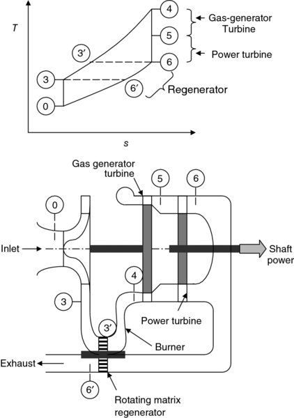
  Calculate the thermal efficiency of a Brayton cycle with cycle pressure ratio of 10, i.e., p₃ / p₀ = 10 and the maximum cycle temperature ratio of T₄/T₀ = 6.5 with and without regeneration.

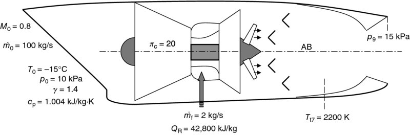
• 4.40 A mixed-exhaust turbofan engine with afterburner is flying at M₀ = 2.5, p₀ = 25 kPa, and T₀ = −35°C. The engine inlet total pressure loss is characterized by π_d = 0.85. The fan pressure ratio is π_f = 1.5 and polytropic efficiency of the fan is e_f = 0.90.

  The flow in the fan duct suffers 1% total pressure loss, i.e., π_fd = 0.99. The compressor pressure ratio and polytropic efficiency are π_c = 12 and e_c = 0.90, respectively. The combustor exit temperature is T_t4 = 1800 K, fuel heating value is Q_R = 42, 800 kJ/kg, total pressure ratio π_b = 0.94, and the burner efficiency is η_b = 0.98. The turbine polytropic efficiency is e_t = 0.80, its mechanical efficiency is η_m = 0.95, and the turbine exit Mach number is M₅ = 0.5. The constant-area mixer suffers a total pressure loss due to friction, which is characterized by π_{M, f} = 0.95. The afterburner is on with T_t7 = 2200 K, Q_{R, AB} = 42, 800 kJ/kg, π_AB-On = 0.92, and afterburner efficiency η_AB = 0.98. The nozzle has a total pressure ratio of π_n = 0.95 and p₉/p₀ = 2.6.

  The gas behavior in the engine is dominated by temperature (in a thermally perfect gas), thus we consider four distinct temperature zones:

  Inlet, fan, and compressor section:    γc = 1.4,     cpc = 1, 004 J/kg · K

  Turbine section:    γt = 1.33, cpt = 1, 152 J/kg · K

  Mixer exit:    γ6M, cp6M (to be calculated based on mixture of gases)

  Afterburner and nozzle section:    γAB = 1.30,     cp, AB = 1, 241 J/kg · K

  Calculate

  1. total pressure and temperature throughout the engine, the fan bypass ratio α, and include the contributions of fuel-to-air ratio in the primary and afterburner, f and f_AB and
  2. engine performance parameters, i.e., TSFC in mg/s/N, specific thrust and cycle efficiencies
• 4.41 An afterburning turbojet engine is in supersonic flight, as shown. The flight condition and cycle parameters are specified. Assuming constant gas properties throughout the engine, calculate
  1. ram drag, D_r in kN
  2. compressor shaft power, ℘_c in MW
  3. fuel-to-air ratio in the primary burner, f
  4. fuel-to-air ratio in the afterburner, f_AB
  5. gas speed at the nozzle throat, V₈, in m/s
  6. exit Mach number, M₉
  7. exit flow area, A₉, in m²

  

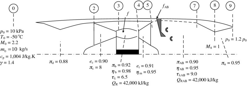
  For Intermediate Steps Calculate These Parameters:

  τr =	τc =	τt =
  πr =	πt =

• 4.42 The thermodynamic state of gas in a ramjet is shown on a T–s diagram.

  

  Assuming constant gas properties, γ = 1.4 and c_p = 1, 004 J/kg · K, calculate

  1. the flight Mach number, M₀
  2. the exhaust Mach number, M₉
  3. the exhaust velocity, V₉, in m/s
• 4.43 The air mass flow rate in a turbojet engine at takeoff is 100 kg/s at standard sea-level conditions (p₀ = 100 kPa, T₀ = 15°C). The fuel-to-air ratio is 0.035 and the nozzle exhaust speed is 1000 m/s. The nozzle is underexpanded with p₉ = 150 kPa. Assuming the nozzle exit temperature is T₉ = 1, 176 K with γ₉ = 1.33 and c_p9 = 1, 156 J/kg · K, calculate
  1. Nozzle exit area, A₉, in m²
  2. Effective exhaust speed, V_9eff, in m/s
  3. Takeoff thrust, F_T.O., in kN
  4. Fuel-specific impulse, I_s, at takeoff in seconds
• 4.44 An afterburning turbojet engine is shown in “wet mode”.

  Calculate

  1. fuel-to-air ratio in the primary burner, f, for Q_R = 42, 000 kJ/kg
  2. turbine exit total temperature, T_t5 (K)
  3. turbine exit total pressure, p_t5, in kPa
  4. fuel-to-air ratio in the afterburner, f_AB, for Q_{R, AB} = 42, 000 kJ/kg
  5. nozzle exit Mach number, M₉

  

• 4.45 The T–s diagram shows the power split between the propeller and the nozzle. Assuming the mass flow rate is = 37 kg/s with γ = 1.33 and c_p = 1, 152 J/kg · K, calculate
  1. ideal power available in station 4.5, ℘_i in MW
  2. LPT exit pressure, p_t5, in kPa
  3. LPT exit temperature, T_t5, in K
  4. LPT power (actual) in MW
  5. nozzle exit velocity, V₉, in m/s, for η_n = 0.95

  

• 4.46 A turboprop aircraft flies at V₀ = 150 m/s and its engine produces 20 kN of propeller thrust and 2 kN of core thrust. For a propeller efficiency of η_prop = 0.85, estimate the engine propulsive efficiency, η_p. [Hint: neglect ]
• 4.47 Consider an afterburning turbojet engine, with afterburner off, as shown.

  The gas is thermally perfect with two zones of “cold” and “hot” described by the gas properties in the compressor and turbine sections as γ_c = 1.4, c_pc = 1, 004 J/kg · K and γ_t = 1.33 and c_pt = 1, 156 J/kg · K, respectively. Assuming the air flow rate is , calculate

  1. D_r, ram drag, in kN and lbf
  2. f, fuel-to-air ratio
  3. T_t5 in K and ^oR
  4. M₉
  5. F_n, net uninstalled thrust in kN and lbf

  

• 4.48 An exhaust nozzle has an inlet total pressure and temperature, p_t7 = 75 kPa and T_t7 = 900 K, respectively. The nozzle exit static pressure is p₉ = 30 kPa where the ambient pressure is p₀ = 20 kPa. Assuming nozzle total pressure ratio is π_n = 0.95, γ_n = 1.33 and c_pn = 1, 156 J/kg · K, calculate
  1. nozzle exhaust speed, V₉, in m/s and fps
  2. the nozzle exhaust speed (in m/s and fps) if the nozzle were perfectly expanded, i.e., p₉ = 20 kPa
• 4.49 An advanced turboprop engine cruises at Mach 0.75 at an altitude where p₀ = 30 kPa and T₀ = 216 K, as shown. The parameters related to each component is identified on the graph, e.g., π_d = 0.98. Also the gas constants representative of the cold and hot section are also specified. The air mass flow rate in the engine is noted to be 50 kg/s. Calculate
  1. total pressure and temperature at the engine face, p_t2 and T_t2, in kPa and K, respectively
  2. total pressure and temperature, p_t3 and T_t3, in kPa and K, respectively
  3. Combustor exit temperature and pressure, T_t4 and p_t4, in K and kPa, respectively
  4. total temperature and pressure at the exit of HPT, T_t4.5 and p_t4.5 in K and kPa respectively
  5. total temperature and pressure at the exit of LPT, T_t5 and p_t5, in K and kPa, respectively
  6. ram drag, D_r, in kN and lbf
  7. propeller thrust, F_prop, in kN and lbf
  8. core nozzle exit Mach number, M₉
  9. core thrust, F_core, in kN and lbf
  10. thrust-specific fuel consumption, TSFC, in mg/s/N (and lbm/hr/lbf)

  

• 4.50 A compressor in a turbojet engine consumes 40 MW of shaft power to handle 100 kg/s of air flow rate and create a compressor total pressure ratio of 15.4. Assuming the inlet condition to the compressor is p_t2 = 100 kPa, T_t2 = 288 K, calculate
  1. the exit total temperature, T_t3, in K
  2. compressor polytropic efficiency, e_c

  Assume γ = 1.4 and c_pc = 1004 J/kg · K

  

• 4.51 A ramjet engine flies at Mach 2 at an altitude where p₀ = 20 kPa and T₀ = 245 K.

  The inlet total pressure recovery is π_d = 0.90 and the combustor exit temperature is T_t4 = 1800 K.

  The fuel heating value is Q_R = 42, 000 kJ/kg the burner efficiency is η_b = 0.98 and the burner total pressure ratio is π_b = 0.95. The nozzle is perfectly expended with π_n = 0.92.

  Assume constant γ of 1.4 and constant c_p of 1004 J/kg · K. Calculate

  1. flight speed, V₀, in m/s and fps
  2. fuel-to-air ratio in the combustor, f
  3. exhaust velocity, V₉, in m/s and fps
  4. ratio of gross thrust to ram drag, F_g/D_r

  

• 4.52 For the separate exhaust turbofan engine shown, calculate: (a) ram drag in kN, (b) fan nozzle gross thrust in kN, (c) net uninstalled thrust in kN, (d) thermal efficiency, (e) propulsive efficiency, (f) thrust specific fuel consumption in mg/s/N.

  

• 4.53 Consider a constant-area mixer, as shown. The mass flow ratio between the cold and hot streams is 3, i.e., . The gas properties are: c_p15 = 1, 004 J/kg · K, γ₁₅ = 1.4 c_p5 = 1, 156 J/kg · K and γ₅ = 1.33. The flow conditions in the inlet to the mixer are:
  

  Assuming the hot gas Mach number is M₅ = 0.4,

  calculate

  1. gas properties at the mixed exit, c_p6M and γ_6M
  2. Mach number of the cold stream, M₁₅
  3. area ratio, A₁₅/A₅
  4. total temperature at the mixed exit, T_t6M in K

  

• 4.54 An afterburning turbojet engine operates at an altitude where the ambient pressure and temperatures are: p₀ = 15 kPa and T₀ = 223 K, respectively. The flight Mach number is M₀ = 2.5 and the ambient air is characterized by c_pc = 1, 004 J/kg · K and γ_c = 1.4. The engine has the following operating parameters and efficiencies: π_d = 0.85, π_c = 6, e_c = 0.92, τ_λ = 7.7, π_b = 0.95, η_b = 0.98, Q_R = 42, 600 kJ/kg, e_t = 0.85, η_m = 0.99, τ_λAB = 10.5, Q_RAB = 42, 600 kJ/kg, π_AB = 0.94, η_AB = 0.97, π_n = 0.95 and p₉ = 15 kPa. Assuming the air flow rate is 50 kg/s in the engine, and gas properties in the turbine and afterburner/nozzle are described by c_pt = 1, 156 J/kg · K, γ_t = 1.33, c_pAB = 1, 243 J/kg · K and γ_AB = 1.30, respectively, calculate
  1. ram drag, D_r, in kN and lbf
  2. compressor shaft power in MW and hp
  3. fuel-to-air ratio, f, in the main burner
  4. turbine discharge p_t5 and T_t5 in kPa and K, respectively
  5. fuel-to-air-ratio in the afterburner, f_ab
  6. nozzle gross thrust in kN and lbf
  7. thrust specific fuel consumption, TSFC, in mg/s/N and lbm/hr/lbf
  8. thermal efficiency, η_th
  9. propulsive efficiency, η_p

  

• 4.55 The total pressures, temperatures and mass flow rates at some stations inside a nonafterburning, mixed-flow turbofan engine, at takeoff, are shown.

  For simplicity of analysis, assume the gas is calorically perfect with constant properties (γ = 1.4 and c_p = 1004 J/kg · K) throughout the engine. Calculate

  1. bypass ratio, α
  2. fuel-to-air ratio, f
  3. mixer exit total temperature, T_t6M, in K
  4. exhaust Mach number, M₈ (note that the exhaust nozzle is of convergent type)
  5. (un-installed) takeoff thrust, F_T.O., in kN and lbf

  

• 4.56 The power turbine in a turboprop engine produces a shaft power of 4.53 MW, working on a gas flow rate of 10.25 kg/s with c_pt = 1, 152 J/kg · K and γ = 1.33. Assuming η_mPT = 0.99, η_gb = 0.99 and η_prop = 0.85 at flight speed of 200 m/s, calculate
  1. the total temperature drop across the power turbine in K
  2. the shaft power delivered to propeller, ℘_prop (MW)
  3. the propeller thrust, F_prop, in kN
• 4.57 A multistage compressor develops a total pressure ratio of π_c = 35 with a polytropic efficiency of e_c = 0.90. The air mass flow rate through the compressor is = 200 kg/s. Assuming γ and c_p remain constant, calculate
  1. Compressor shaft power, ℘_c, in MW
  2. Flow area in 2, i.e., A₂, in m²
  3. Density of air in station 3, ρ₃, in kg/m³ [note: the axial velocity at the compressor exit, V₃ = V₂]
  4. The nondimensional entropy rise across the compressor, Δs/R

  

• 4.58 A ramjet in flight is shown. The inlet total pressure recovery is π_d = 0.80 and the nozzle is underexpanded.

  Calculate

  1. ram temperature and pressure ratios, τ_r and π_r
  2. the total temperature at the combustor exit, T_t4, in K and the corresponding τ_λ
  3. exhaust velocity, V₉, in m/s
  4. pressure thrust as a fraction of nozzle momentum thrust, i.e.,
  5. the propulsive efficiency of the ramjet, η_p (note that the nozzle is not perfectly expanded, so you need to calculate V_9eff)
  6. thrust-specific fuel consumption, TSFC, in mg/s/N and lbm/hr/lbf

  

• 4.59 A separate exhaust turbofan engine has convergent nozzles with the following parameters:
  • M₀ = 0.85
  • p₀ = 30 kPa, T₀ = 240 K, γ_c = 1.4, c_pc = 1004 J/kg · K
  • π_d = 0.98
  • π_f = 1.55, e_f = 0.90
  • π_fn = 0.97

  Calculate

  1. fan exit total pressure, p_t13, in kPa
  2. fan exit total temperature, T_t13, in K
  3. exit Mach number, M₁₉
  4. nozzle exit static pressure, p₁₉ (or p₁₈), in kPa
  5. exhaust speed, V₁₉ (or V₁₈), in m/s
  6. effective exhaust velocity, V_{19 eff}, in m/s

  

• 4.60 A turboprop uses a power split of 0.96 between the power turbine and the exhaust nozzle, i.e. α = 0.96. The adiabatic efficiency of the LPT (or power turbine) is η_LPT = 0.88. The flow at the inlet of the LPT has p_t4.5 = 99 kPa and T_t4.5 = 845 K. The nozzle adiabatic efficiency is η_n = 0.95.

  Calculate

  1. the shaft power per unit mass flow rate of the LPT in kJ/kg
  2. the exhaust velocity, V₉, in m/s

  

• 4.61 An un-cooled turbine has entrance and exit flow conditions: p_t4 = 2.5 MPa, T_t4 = 1760 K, T_t5 = 1000 K. The gas mass flow rate in the turbine is and the turbine polytropic efficiency is e_t = 0.85. Assuming γ_t = 1.33 and c_pt = 1156 J/kg · K, calculate
  1. turbine exit total pressure, p_t5, in kPa
  2. turbine shaft power in MW
  3. turbine adiabatic efficiency, η_t

  

• 4.62 The flow condition at the entrance to a constant-area mixer is that the mass flow rate from the fan side, and the mass flow rate from the core is . The entrance total temperatures are T_t15 = 360 K and T_t5 = 895 K. The cold and hot streams have γ_c = 1.4, c_pc = 1004 J/kg · K, γ_t = 1.33 and c_pt = 1156 J/kg · K. Calculate
  1. the gas properties at the mixer exit, γ_6M and c_p6M
  2. the mixer exit total temperature, T_t6M, in K

  

• 4.63 A ramjet is shown in supersonic flight. The inlet total pressure recovery is π_d = 0.90 and the nozzle is underexpanded (note that p₉ ≠ p₀).

  Calculate

  1. ram temperature and pressure ratios, τ_r and π_r
  2. the total temperature at the combustor exit, T_t4, in K and the corresponding τ_λ
  3. Exhaust velocity, V₉, in m/s
  4. pressure thrust as a fraction of nozzle momentum thrust, i.e.,
  5. the propulsive efficiency of the ramjet, η_p (note that the nozzle is not perfectly expanded, so you need to calculate V_9eff)
  6. thrust-specific fuel consumption, TSFC, in mg/s/N and lbm/hr/lbf
• 4.64 A turbojet engine is flying at Mach 1.6, with ambient pressure, p₀ = 25 kPa and temperature, T₀ = 230 K. The inlet total pressure recovery is π_d = 0.85 and the compressor pressure ratio is π_c = 12 with e_c = 0.90.

  Assuming the air flow rate is 50 kg/s, calculate

  1. ram drag in kN
  2. compressor exit total pressure, p_t3, in kPa
  3. compressor shaft power, ℘_c, in MW
  4. inlet adiabatic efficiency, η_d

  

• 4.65 A turboprop is in a Mach 0.80 flight at an altitude where p₀ = 22 kPa and temperature is T₀ = 245 K with γ_c = 1.4 and c_pc = 1004 J/kg · K. The inlet total pressure loss is 3% of flight dynamic pressure, i.e., p_t0-p_t2 = 0.03 q₀. The compressor pressure ratio is π_c = 35 and its polytropic efficiency is e_c = 0.90. The combustor achieves an exit total temperature of T_t4 = 1, 650 K while burning a hydrocarbon fuel with an ideal heating value of 42, 000 kJ/kg, at a burner efficiency of η_b = 0.99 and a total pressure ratio π_b = 0.95. The gas in the hot section is characterized by γ_t = 1.33 and c_pt = 1, 152 J/kg · K. The high-pressure turbine has η_mHPT = 0.995 and a polytropic efficiency of e_HPT = 0.85. The power split parameter between the low-pressure turbine and the nozzle is α = 0.85. The low-pressure turbine has adiabatic and mechanical efficiencies of η_LPT = 0.90 and η_{m, LPT} = 0.995 respectively. The propeller is gearbox-driven with η_gb = 0.995 and the propeller efficiency is η_prop = 0.80. Assuming the nozzle is perfectly expanded, p₉ = p₀, and η_n = 0.96, calculate:
  1. flight dynamic pressure, q₀, in kPa
  2. compressor discharge (total) temperature, T_t3 in K
  3. the fuel-to-air ratio, f, in the burner
  4. the total pressure and temperature at the exit of HPT, i.e., p_t4.5 (in kPa) and T_t4.5 in K
  5. the total pressure and temperature at the exit of the LPT, p_t5 in kPa and T_t5 in K
  6. the nozzle exit Mach number, M₉
  7. the nozzle exit velocity, V₉
  8. the propeller thrust, F_prop in kN

  

• 4.66 A ramjet flies at Mach 2.2 at an altitude where the speed of sound is a₀ = 294 m/s and the pressure is p₀ = 20 kPa. The air is characterized as perfect gas with γ = 1.4 and R = 287 J/kg · K. The inlet total pressure recovery is π_d = 0.90, combustor losses are characterized by π_b = 0.92, η_b = 0.99 and the nozzle total pressure loss parameter is π_n = 0.94. Assuming nozzle is perfectly expanded, combustor exit temperature is T_t4 = 2, 000 K, fuel heating value is Q_R = 42, 600 kJ/kg, and gas properties (γ and R) remain constant in the ramjet, calculate
  1. enthalpy ratio, τ_λ
  2. fuel-to-air ratio, f
  3. exhaust speed, V₉, in m/s
  4. non-dimensional specific thrust,
  5. propulsive efficiency, η_p
  6. thermal efficiency, η_th

  

• 4.67 A separate-flow turbofan engine is shown at cruise condition. The flight condition, air and fuel flow rates, nozzle exit conditions and fuel properties are all labeled in the schematic drawing (Figure P4.67). The primary and fan nozzles are of convergent type and both are choked, as shown.

  Calculate

  1. ram drag in kN and lbf
  2. fan nozzle exit area, A₁₈, in m² and ft²
  3. fan nozzle gross thrust in kN and lbf
  4. core nozzle exit area, A₈, in m² and ft²
  5. core nozzle gross thrust in kN and lbf
  6. TSFC in mg/s/N and lbm/hr/lbf
  7. fan total temperature ratio, τ_f
  8. fan total pressure ratio, π_f, if the fan polytropic efficiency is e_f = 0.90
  9. fan nozzle effective exhaust speed, V_{18, eff}, in m/s and fps
  10. core nozzle effective exhaust speed, V_{8, eff}, in m/s and fps
  11. engine propulsive efficiency, η_p (%)
  12. engine thermal efficiency, η_th (%)

  

• 4.68 A ramjet is shown at Mach 2.4 flight at an altitude where p₀ = 25 kPa and T₀ = 240 K. The inlet total pressure recovery is 90%. The air and fuel mass flow rates are 100 and 5.0 kg/s respectively, as shown.

  The nozzle total pressure ratio is 95% and it is perfectly expanded. The gas properties for the cold and hot sections of the engine are: γ_c = 1.4, c_pc = 1, 004 J/kgK and γ_t = 1.3, c_pt = 1, 243 J/kg · K, respectively. Calculate

  1. ram drag, D_r, in kN and lbf
  2. combustor exit total pressure, p_t4, in kPa
  3. combustor exit total temperature, T_t4, in K
  4. nozzle exit Mach number and velocity, M₉ and V₉, in m/s
  5. nozzle gross thrust, F_g, in kN and lbf
  6. thrust-specific fuel consumption, TSFC, in mg/s/N and lbm/hr/lbf
  7. engine thermal efficiency, η_th
  8. engine propulsive efficiency, η_p