
Chapter 2
A First Approach for Modeling Time Series of Counts: The Thinning-based INAR(1) Model
As a first step towards the analysis and modeling of count time series, we consider an integer-valued counterpart to the conventional first-order autoregressive model, the INAR(1) model of McKenzie (1985). This constitutes a rather simple and easily interpretable Markov model for stationary count processes, but it is also quite powerful due to its flexibility and expandability. In particular, it allows us to introduce some basic approaches for parameter estimation, model diagnostics and statistical inference. These are used in an analogous way also for the more advanced models discussed in Chapters 3–5. The presented models and methods are illustrated with a data example in Section 2.5.
To prepare for our discussion about count time series, however, we start in Section 2.1 with a brief introduction to the notation used in this book, and with some remarks regarding characteristic features of count distributions in general (without a time aspect).
2.0 Preliminaries: Notation and Characteristics of Count Distributions
In contrast to the subsequent sections, here we remove any time aspects and look solely at separate random variables and their distributions. The first aim of this preliminary section is to acquaint the reader with the basic notation used in this book. The second one is to briefly highlight characteristic features of count distributions, which will be useful in identifying appropriate models for a given scenario or dataset. To avoid a lengthy and technical discussion, detailed definitions and surveys of specific distributions are avoided here but are provided in Appendix A instead.
Count data express the number of certain units or events in a specified context. The possible outcomes are contained in the set of non-negative integers, ![]() . These outcomes are not just used as labels; they arise from counting and are hence quantitative (ratio scale). Accordingly, we refer to a quantitative random variable
. These outcomes are not just used as labels; they arise from counting and are hence quantitative (ratio scale). Accordingly, we refer to a quantitative random variable ![]() as a count random variable if its range is contained in the set of non-negative integers,
as a count random variable if its range is contained in the set of non-negative integers, ![]() . Some examples of random count phenomena are:
. Some examples of random count phenomena are:
- the number of emails one gets at a certain day (unlimited range
 )
) - the number of occupied rooms in a hotel with
 rooms (finite range
  )
) - the number of trials until a certain event happens (unlimited range
 ).
).
A common way of expressing location and dispersion of a count random variable ![]() is to use mean and variance, denoted as
is to use mean and variance, denoted as
The definition and notation of more general types of moments are summarized in Table 2.1; note that ![]() is the mean of
is the mean of ![]() , and
, and ![]() is the variance of
is the variance of ![]() .
.
Table 2.1 Definition and notation of moments of a count random variable ![]()
| For |
While such moments give insight into specific features of the distribution of ![]() , the complete distribution is uniquely defined by providing its probability mass function (pmf), which we abbreviate as
, the complete distribution is uniquely defined by providing its probability mass function (pmf), which we abbreviate as
Similarly, ![]() denotes the cumulative distribution function (cdf). An alternative way of completely characterizing a count distribution is to derive an appropriate type of generating function; the most common types are summarized in Table 2.2. The probability generating function (pgf), for instance, encodes the pmf of the distribution, but it also allows derivation of the factorial moments: the
denotes the cumulative distribution function (cdf). An alternative way of completely characterizing a count distribution is to derive an appropriate type of generating function; the most common types are summarized in Table 2.2. The probability generating function (pgf), for instance, encodes the pmf of the distribution, but it also allows derivation of the factorial moments: the ![]() th derivative satisfies
th derivative satisfies ![]() ; in particular,
; in particular, ![]() . The coefficients
. The coefficients ![]() of
of ![]() are referred to as the cumulants. Particular cumulants are
are referred to as the cumulants. Particular cumulants are
that is, ![]() is the skewness and
is the skewness and ![]() the excess of the distribution. The coefficients
the excess of the distribution. The coefficients ![]() of the factorial-cumulant generating function (fcgf) are referred to as the factorial cumulants.
of the factorial-cumulant generating function (fcgf) are referred to as the factorial cumulants.
Table 2.2 Definition and notation of generating functions of a count r. v. ![]()
| Generating functions of |
|
| Probability (pgf) | |
| Moment (mgf) | |
| Cumulant (cgf) | |
| Factorial-cumulant (fcgf) | |
A number of parametric models for count distributions are available in the literature. See Appendix A for a brief survey. There, the models are sorted according to the dimension of their ranges (univariate vs. multivariate), and according to size: in some applications, there exists a fixed upper bound ![]() that can never be exceeded, so the range is of finite size, taking the form
that can never be exceeded, so the range is of finite size, taking the form ![]() ; otherwise, we have the unlimited range
; otherwise, we have the unlimited range ![]() .
.
Distributions for the case of ![]() being a univariate count random variable with the unlimited range
being a univariate count random variable with the unlimited range ![]() are presented in Appendix A.1. There, the Poisson distribution has an outstanding position (similar to the normal distribution in the continuous case) and often serves as the benchmark for the modeling of count data. One of its main characteristics is the equidispersion property, which means that its variance is always equal to its mean. If we define the (Poisson) index of dispersion as
are presented in Appendix A.1. There, the Poisson distribution has an outstanding position (similar to the normal distribution in the continuous case) and often serves as the benchmark for the modeling of count data. One of its main characteristics is the equidispersion property, which means that its variance is always equal to its mean. If we define the (Poisson) index of dispersion as

for a random variable ![]() with mean
with mean ![]() and variance
and variance ![]() , then the Poisson distribution always satisfies
, then the Poisson distribution always satisfies ![]() . Values for
. Values for ![]() deviating from 1, in turn, express a violation of the Poisson model:
deviating from 1, in turn, express a violation of the Poisson model: ![]() indicates an overdispersed distribution, such as the negative binomial distribution from Example A.1.4 or Consul's generalized Poisson distribution from Example A.1.6.
indicates an overdispersed distribution, such as the negative binomial distribution from Example A.1.4 or Consul's generalized Poisson distribution from Example A.1.6. ![]() expresses underdispersion, for example in the Good distribution from Example A.1.7 or the PL distribution from Example A.1.8.
expresses underdispersion, for example in the Good distribution from Example A.1.7 or the PL distribution from Example A.1.8.
Figure 2.1 illustrates the difference between the equidispersed Poisson distribution (black) and the overdispersed negative binomial distribution (NB; gray) or generalized Poisson distribution (GP; light gray), respectively. All distributions are calibrated to the same mean ![]() , but the plotted NB and GP models have dispersion indices
, but the plotted NB and GP models have dispersion indices ![]() (that is, 100% overdispersion). It can be seen that both the NB and GP models have more probability mass for values
(that is, 100% overdispersion). It can be seen that both the NB and GP models have more probability mass for values ![]() , but also the zero probability is increased (Poi:
, but also the zero probability is increased (Poi: ![]() , NB:
, NB: ![]() , GP:
, GP: ![]() ); the latter phenomenon is discussed in more detail below.
); the latter phenomenon is discussed in more detail below.

Figure 2.1 Count distributions with  : Poisson in black; NB and GP distributions (both with 100% overdispersion) in gray.
Figure 2.2, in contrast, illustrates the effect of underdispersion, compared to the equidispersed Poisson distribution (black) with mean ![]() : the plotted Good distribution (gray; Example A.1.7) and the PL
: the plotted Good distribution (gray; Example A.1.7) and the PL![]() distribution (light gray; Example A.1.8) both have mean
distribution (light gray; Example A.1.8) both have mean ![]() and dispersion index
and dispersion index ![]() (that is, 50% underdispersion). These underdispersed models concentrate most of their probability mass on the values 1 and 2. In particular, the zero probability is much lower than in the Poisson case (Poi:
(that is, 50% underdispersion). These underdispersed models concentrate most of their probability mass on the values 1 and 2. In particular, the zero probability is much lower than in the Poisson case (Poi: ![]() , Good:
, Good: ![]() , PL
, PL![]() :
: ![]() ).
).

Figure 2.2 Count distributions with  : Poisson in black; Good and PL
 distributions (both with
  underdispersion) in gray.
When discussing Figures 2.1 and 2.2, it becomes clear that another characteristic property of the Poisson distribution is the probability of observing a zero, ![]() . Hence, the zero index (Puig & Valero, 2006)
. Hence, the zero index (Puig & Valero, 2006)

as a function of mean ![]() and zero probability
and zero probability ![]() , takes the value 0 for the Poisson distribution, but may differ otherwise. Values
, takes the value 0 for the Poisson distribution, but may differ otherwise. Values ![]() indicate zero inflation (excess of zeros with respect to a Poisson distribution), while
indicate zero inflation (excess of zeros with respect to a Poisson distribution), while ![]() refers to zero deflation. A useful approach for modifying a distribution's zero probability is described in Example A.1.9.
refers to zero deflation. A useful approach for modifying a distribution's zero probability is described in Example A.1.9.
The previous discussion as well as the definition of the indices (2.1) and (2.2) are for distributions having an unlimited range ![]() . However, as mentioned before, sometimes the range is finite,
. However, as mentioned before, sometimes the range is finite, ![]() with fixed upper bound
with fixed upper bound ![]() . In such a case, the binomial distribution (Example A.2.1 in Appendix A.2) plays a central role. If we characterize its dispersion behavior in terms of the index of dispersion (2.1), the binomial distribution is underdispersed. However, since we are concerned with a different type of random phenomenon anyway – one with a finite range – it is more appropriate to evaluate the dispersion behavior in terms of the so-called binomial index of dispersion, defined by
. In such a case, the binomial distribution (Example A.2.1 in Appendix A.2) plays a central role. If we characterize its dispersion behavior in terms of the index of dispersion (2.1), the binomial distribution is underdispersed. However, since we are concerned with a different type of random phenomenon anyway – one with a finite range – it is more appropriate to evaluate the dispersion behavior in terms of the so-called binomial index of dispersion, defined by

for a random variable ![]() with range
with range ![]() , mean
, mean ![]() and variance
and variance ![]() . See also Hagmark (2009), and note that
. See also Hagmark (2009), and note that ![]() for
for ![]() . In view of this index, the binomial distribution always satisfies
. In view of this index, the binomial distribution always satisfies ![]() , while a distribution with
, while a distribution with ![]() is said to exhibit extra-binomial variation. An example is the beta-binomial distribution from Example A.2.2. For illustration, Figure 2.3 shows a binomial and a beta-binomial distribution with range
is said to exhibit extra-binomial variation. An example is the beta-binomial distribution from Example A.2.2. For illustration, Figure 2.3 shows a binomial and a beta-binomial distribution with range ![]() and the unique mean 6, but with the beta-binomial distribution exhibiting a strong degree of extra-binomial variation (420%).
and the unique mean 6, but with the beta-binomial distribution exhibiting a strong degree of extra-binomial variation (420%).

Figure 2.3 Binomial distribution  in black, and corresponding beta-binomial distribution with
  (
( ) in gray.
Although this book, as an introductory course in discrete-valued time series, mainly focusses on the univariate case, in some places a brief account of possible multivariate generalizations is also provided. Therefore, Appendix A.3 presents multivariate extensions to some basic count models such as the Poisson or negative binomial. These extensions preserve the respective univariate distribution for their marginals, but they induce cross-correlation between the components of the multivariate count vector. An example is plotted in Figure 2.4. The bivariate Poisson (Example A.3.1) and negative binomial distribution (Example A.3.2) shown there are adjusted to give the same mean ![]() and the same cross-correlation
and the same cross-correlation ![]() , but the negative binomial model obviously shows more dispersion in both components: the dispersion indices are 2 and
, but the negative binomial model obviously shows more dispersion in both components: the dispersion indices are 2 and ![]() , respectively.
, respectively.
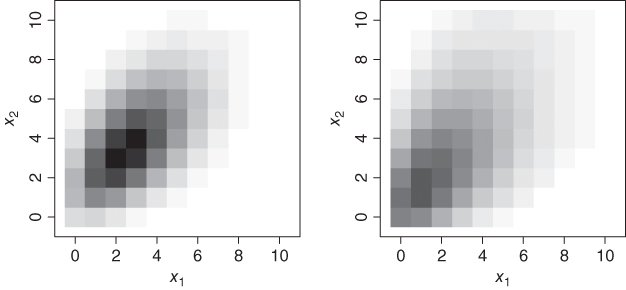
Figure 2.4 Bivariate Poisson (left) and negative binomial distribution (right) with mean  and cross-correlation
  .
.
One of the multivariate count distributions, the multinomial distribution from Example A.3.3, will be of importance in Part II's consideration of categorical time series; see also the discussion in the appendix. The connection to compositional data (Remark A.3.4) is briefly mentioned in this context.
2.1 The INAR(1) Model for Time-dependent Counts
In 1985, in issues 4 and 5 of volume 21 of the Water Resources Bulletin (nowadays the Journal of the American Water Resources Association), a series of papers about time series analysis appeared, and were also published separately by the American Water Resources Association as the monograph Time Series Analysis in Water Resources (edited by K.W. Hipel). One of these papers, “Some simple models for discrete variate time series” by McKenzie (1985), introduced a number of AR(1)-like models for count time series. At this point, it is important to note that the conventional AR(1) recursion, ![]() , cannot be applied to count processes: even if the innovations
, cannot be applied to count processes: even if the innovations ![]() are assumed to be integer-valued with range
are assumed to be integer-valued with range ![]() , the observations
, the observations ![]() would still not be integer-valued, since the multiplication “
would still not be integer-valued, since the multiplication “![]() ” does not preserve the discrete range (the so-called multiplication problem). Therefore, the idea behind McKenzie's new models was to use different mechanisms for “reducing”
” does not preserve the discrete range (the so-called multiplication problem). Therefore, the idea behind McKenzie's new models was to use different mechanisms for “reducing” ![]() . One such mechanism is the binomial thinning operator (Steutel & van Harn, 1979), which was used to define the integer-valued AR(1) model, or INAR(1) model for short. The binomial AR(1) model, discussed in Section 3.3, was also introduced in this context.
. One such mechanism is the binomial thinning operator (Steutel & van Harn, 1979), which was used to define the integer-valued AR(1) model, or INAR(1) model for short. The binomial AR(1) model, discussed in Section 3.3, was also introduced in this context.
It seems that McKenzie's paper was overlooked in the beginning, possibly because the Water Resources Bulletin was not a typical outlet for time series papers: two years later, the INAR(1) model was proposed again by Al-Osh & Alzaid (1987), but now in the Journal of Time Series Analysis. Eventually, McKenzie's paper and the one by Al-Osh & Alzaid, turned out to be groundbreaking for the field of count time series, initiating innumerable research papers about thinning-based time series models (some of them are presented in Section 3) and attracting more and more attention to discrete-valued time series.
We shall now examine the important stochastic properties as well as relevant special cases of the INAR(1) model in great detail. This will allow for more compact presentations of many other models in the later chapters of this book.
2.1.1 Definition and Basic Properties
A way of avoiding the multiplication problem, as sketched above, is to use the probabilistic operation of binomial thinning (Steutel & van Harn, 1979), sometimes also referred to as binomial subsampling (Puig & Valero, 2007). If ![]() is a discrete random variable with range
is a discrete random variable with range ![]() and if
and if ![]() , then the random variable
, then the random variable ![]() is said to arise from
is said to arise from ![]() by binomial thinning, and the
by binomial thinning, and the ![]() are referred to as the counting series. They are i.i.d. binary random variables with
are referred to as the counting series. They are i.i.d. binary random variables with ![]() , which are also independent of
, which are also independent of ![]() . So by construction,
. So by construction, ![]() can only lead to integer values between 0 and
can only lead to integer values between 0 and ![]() . The boundary values
. The boundary values ![]() and
and ![]() might be included in this definition by setting
might be included in this definition by setting ![]() and
and ![]() . Since each
. Since each ![]() satisfies
satisfies ![]() (see Example A.2.1), and since the binomial distribution is additive,
(see Example A.2.1), and since the binomial distribution is additive, ![]() has a conditional binomial distribution given the value of
has a conditional binomial distribution given the value of ![]() ; that is,
; that is, ![]() . In particular, using the law of total expectation, it follows that
. In particular, using the law of total expectation, it follows that

So the binomial thinning ![]() and the multiplication
and the multiplication ![]() have the same mean, which motivates us to use binomial thinning within a modified AR(1) recursion. However, they differ in many other properties; in particular, the multiplication is not a random operation. As an example, the law of total variance implies that
have the same mean, which motivates us to use binomial thinning within a modified AR(1) recursion. However, they differ in many other properties; in particular, the multiplication is not a random operation. As an example, the law of total variance implies that

so we have ![]() .
.
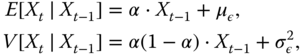
For the interpretation of the binomial thinning operation, consider a population of size ![]() at a certain time
at a certain time ![]() . If we observe the same population at a later time,
. If we observe the same population at a later time, ![]() , then the population may have shrunk, because some of the individuals had died between times
, then the population may have shrunk, because some of the individuals had died between times ![]() and
and ![]() . If the individuals survive independently of each other, and if the probability of surviving from
. If the individuals survive independently of each other, and if the probability of surviving from ![]() to
to ![]() is equal to
is equal to ![]() for all individuals, then the number of survivors is given by
for all individuals, then the number of survivors is given by ![]() .
.
Using the random operator “![]() ”, McKenzie (1985) and Al-Osh & Alzaid (1987) defined the INAR(1) process in the following way.
”, McKenzie (1985) and Al-Osh & Alzaid (1987) defined the INAR(1) process in the following way.
Note that it would be more correct to write “![]() ” in the above recursion to emphasize the fact that the thinning is realized at each time
” in the above recursion to emphasize the fact that the thinning is realized at each time ![]() anew. However, for the sake of readability, the time index is avoided.
anew. However, for the sake of readability, the time index is avoided.
The INAR(1) recursion of Definition 2.1.1.1 can be interpreted as follows (Al-Osh & Alzaid, 1987):
The INAR(1) process is a homogeneous Markov chain with the 1-step transition probabilities given by (McKenzie, 1985; Al-Osh & Alzaid, 1987):

For conditional mean and variance, we have (Alzaid & Al-Osh, 1988):
which are both linear functions of ![]() . For the derivation of (2.5) and (2.6), note that
. For the derivation of (2.5) and (2.6), note that ![]() and
and ![]() are independent according to Definition 2.1.1.1. Since the conditional mean is linear in
are independent according to Definition 2.1.1.1. Since the conditional mean is linear in ![]() , the INAR(1) model belongs to the class of conditional linear AR(1) models, or CLAR(1), as discussed by Grunwald et al. (2000). Note that the conditional variance differs from the AR(1) case as it varies with time (conditional heteroscedasticity; see the discussion before Definition B.4.1.1).
, the INAR(1) model belongs to the class of conditional linear AR(1) models, or CLAR(1), as discussed by Grunwald et al. (2000). Note that the conditional variance differs from the AR(1) case as it varies with time (conditional heteroscedasticity; see the discussion before Definition B.4.1.1).
Let us now assume that the INAR(1) process is even stationary (Definition B.1.3). Conditions for guaranteeing a stationary solution of the INAR(1) recursion are discussed below. If we have given the innovations' distribution in terms of the pgf, then the observations' stationary marginal distribution is determined by the equation (Alzaid & Al-Osh, 1988):
See also the discussion in Section 2.1.3 below. Note that (2.7) is again obtained by applying the law of total expectation, as

Equation 2.7 can be used to determine the marginal moments or cumulants of ![]() ; see Weiß (2013a). In particular, if
; see Weiß (2013a). In particular, if ![]() , mean and variance are given by
, mean and variance are given by

where ![]() refers to the index of dispersion (2.1). It implies that
refers to the index of dispersion (2.1). It implies that ![]() is over-/equi-/underdispersed iff
is over-/equi-/underdispersed iff ![]() is over-/equi-/underdispersed; that is, the dispersion behavior of the observations is determined by the one of the innovations.
is over-/equi-/underdispersed; that is, the dispersion behavior of the observations is determined by the one of the innovations.
The autocorrelation function (ACF; see Definition B.1.1) ![]() of a stationary INAR(1) process equals
of a stationary INAR(1) process equals ![]() (McKenzie, 1985; Al-Osh & Alzaid, 1987); that is, it is of AR(1) type. Expressions for higher-order joint moments in
(McKenzie, 1985; Al-Osh & Alzaid, 1987); that is, it is of AR(1) type. Expressions for higher-order joint moments in ![]() are provided by Schweer & Weiß (2014).
are provided by Schweer & Weiß (2014).
A further useful relationship of INAR(1) models is to certain queue length processes with an infinite number of servers. For instance, the Poisson INAR(1) model, which will be discussed in Section 2.1.2, corresponds to an ![]() queue observed at integer times (McKenzie, 2003).
queue observed at integer times (McKenzie, 2003).
2.1.2 The Poisson INAR(1) Model
The most popular instance of the INAR(1) family is the Poisson INAR(1) model, which was introduced by McKenzie (1985) and Al-Osh & Alzaid (1987). Here, it is assumed that the innovations ![]() are i.i.d. according to the Poisson distribution
are i.i.d. according to the Poisson distribution ![]() , such that
, such that ![]() . Since all
. Since all ![]() are truly positive, this also holds for all transition probabilities
are truly positive, this also holds for all transition probabilities ![]() from (2.5). Consequently, a Poisson INAR(1) process is an irreducible and aperiodic Markov chain (see Appendix B.2.2), such that Remark 2.1.1.2 implies a unique stationary marginal distribution for
from (2.5). Consequently, a Poisson INAR(1) process is an irreducible and aperiodic Markov chain (see Appendix B.2.2), such that Remark 2.1.1.2 implies a unique stationary marginal distribution for ![]() .
.
It is well known that this stationary marginal distribution is also a Poisson distribution, ![]() with
with ![]() . This follows from two important invariance properties of the Poisson distribution
. This follows from two important invariance properties of the Poisson distribution
- the invariance with respect to binomial thinning; that is, if
 , then
- the additivity; that is, if
 ,
,  and both are independent, then
  ; see Example A.1.1.
Knowing both the conditional and the marginal distribution, we are able to easily simulate a stationary Poisson INAR(1) process – just initialize by ![]() – and the full likelihood function is also directly available; see Remark B.2.1.2 and Example 2.2.2.1 below. Furthermore, the property of having both the observations and the innovations within the same distribution family is analogous to the case of a Gaussian AR(1) model. Another similarity between Poisson INAR(1) and Gaussian AR(1) processes, which distinguishes these special instances from other INAR(1) or AR(1) processes, respectively, is time reversibility, see Schweer (2015).
– and the full likelihood function is also directly available; see Remark B.2.1.2 and Example 2.2.2.1 below. Furthermore, the property of having both the observations and the innovations within the same distribution family is analogous to the case of a Gaussian AR(1) model. Another similarity between Poisson INAR(1) and Gaussian AR(1) processes, which distinguishes these special instances from other INAR(1) or AR(1) processes, respectively, is time reversibility, see Schweer (2015).

Figure 2.5 Simulated sample paths of Poisson INAR(1) processes with  and (a)
  , (b)
, (b)  , see Example 2.1.2.1.
2.1.3 INAR(1) Models with More General Innovations
The INAR(1) model becomes particularly simple if the innovations are chosen to be Poisson distributed; see Section 2.1.2. But much more flexibility in terms of marginal distributions is possible. One option is to select an appropriate model for the observations ![]() and then compute the corresponding innovations' distribution from (2.7); see McKenzie (1985) and the details below. Another option is to choose the distribution of the innovations
and then compute the corresponding innovations' distribution from (2.7); see McKenzie (1985) and the details below. Another option is to choose the distribution of the innovations ![]() in order to obtain certain properties for the observations' distribution (Al-Osh & Alzaid, 1987; Alzaid & Al-Osh, 1988); this approach usually simplifies the computation of the transition probabilities (2.5). Generally, see (2.8), the dispersion behavior of the observations is easily controlled by that of the innovations. Also, the probability for observing a zero is influenced by the innovations: since the zero probability just equals
in order to obtain certain properties for the observations' distribution (Al-Osh & Alzaid, 1987; Alzaid & Al-Osh, 1988); this approach usually simplifies the computation of the transition probabilities (2.5). Generally, see (2.8), the dispersion behavior of the observations is easily controlled by that of the innovations. Also, the probability for observing a zero is influenced by the innovations: since the zero probability just equals ![]() , (2.7) implies that
, (2.7) implies that

see Jazi et al. (2012). So we are not only able to generate over- or underdispersion, but also zero inflation or deflation (see Equation 2.2).
Let us now look at special instances. The most natural extension beyond Poisson distributions is to consider the family of discrete self-decomposable (DSD) distributions for ![]() (Steutel & van Harn, 1979), which includes, for example, the negative binomial (NB) distribution (see Example A.1.4) as well as the generalized Poisson (GP) distribution (Example A.1.6); see Zhu & Joe (2003) and Weiß (2008a) for more details. Here, a distribution is said to be DSD if its pgf satisfies:
(Steutel & van Harn, 1979), which includes, for example, the negative binomial (NB) distribution (see Example A.1.4) as well as the generalized Poisson (GP) distribution (Example A.1.6); see Zhu & Joe (2003) and Weiß (2008a) for more details. Here, a distribution is said to be DSD if its pgf satisfies:

that is, the coefficients of its power series expansion must be non-negative and add up to 1. In view of (2.7) (2.10) implies that DSD distributions are the marginal distributions of an INAR(1) process that can be preserved for any choice of ![]() ; the corresponding innovations' pgf is then given by (2.10). Note that any DSD distribution is also infinitely divisible (while the reverse statement does not hold). In other words, it is a particular type of compound Poisson (CP) distribution according to Example A.1.2. As a result, if it is not the Poisson distribution, a DSD distribution is overdispersed and zero-inflated.
; the corresponding innovations' pgf is then given by (2.10). Note that any DSD distribution is also infinitely divisible (while the reverse statement does not hold). In other words, it is a particular type of compound Poisson (CP) distribution according to Example A.1.2. As a result, if it is not the Poisson distribution, a DSD distribution is overdispersed and zero-inflated.
If we do not insist on having the same marginal distribution for all ![]() , we can simply select a distribution for the innovations, thus controlling dispersion or zero behavior of the observations; see the above discussion. Following this strategy, the most straightforward extension is to choose
, we can simply select a distribution for the innovations, thus controlling dispersion or zero behavior of the observations; see the above discussion. Following this strategy, the most straightforward extension is to choose ![]() to be CP-distributed, since then, as in the Poisson case, the observations are also CP-distributed, a characteristic which follows from the invariance properties described next (Schweer & Weiß, 2014).
to be CP-distributed, since then, as in the Poisson case, the observations are also CP-distributed, a characteristic which follows from the invariance properties described next (Schweer & Weiß, 2014).
In fact, Puig & Valero (2007) showed that a count model being parametrized by its ![]() first factorial cumulants
first factorial cumulants ![]() is closed under addition and under binomial thinning iff it has a
is closed under addition and under binomial thinning iff it has a ![]() distribution. These invariance properties lead to the definition of the compound Poisson INAR(1) or CP-INAR(1) model.
distribution. These invariance properties lead to the definition of the compound Poisson INAR(1) or CP-INAR(1) model.
A widely used special instance of the CP-INAR(1) model is the NB-INAR(1) model, in which the innovations are negatively binomially distributed (Example A.1.4). Note that the marginal distribution of ![]() is not an NB distribution, but just another type of
is not an NB distribution, but just another type of ![]() distribution.
distribution.
As mentioned above, a (non-Poisson) CP-INAR(1) model always has an overdispersed and zero-inflated marginal distribution. If, however, underdispersion or zero-deflation are required, then we have to choose the innovations from outside the CP family. Models with underdispersed innovations ![]() (following the Good distribution in Example A.1.7 or the PL distribution in Example A.1.8), and therefore with underdispersed observations
(following the Good distribution in Example A.1.7 or the PL distribution in Example A.1.8), and therefore with underdispersed observations ![]() according to (2.8), are discussed by Weiß (2013a). Jazi et al. (2012) consider zero-modified innovations (Example A.1.9).
according to (2.8), are discussed by Weiß (2013a). Jazi et al. (2012) consider zero-modified innovations (Example A.1.9).

Figure 2.6 Marginal distribution ( ) of NB-INAR(1) model
  in black, and of Poisson INAR(1) model
 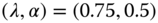 in gray.
2.2 Approaches for Parameter Estimation
The INAR(1) model is determined by the thinning parameter ![]() on the one hand, and by further parameters characterizing the marginal distribution of the observations or innovations, respectively, on the other hand. Given the time series data
on the one hand, and by further parameters characterizing the marginal distribution of the observations or innovations, respectively, on the other hand. Given the time series data ![]() , the task is to estimate the value of these parameters.
, the task is to estimate the value of these parameters.
2.2.1 Method of Moments
Let ![]() be a time series stemming from a stationary INAR(1) process. A quite pragmatic approach for parameter estimation is the method of moments (MM). Here, the idea is to select appropriate moment relations such that the true model parameters can be obtained by solving the resulting system of equations. For parameter estimation, the true moments are replaced by the corresponding sample moments (see Definition B.1.4), thus leading to the MM estimates.
be a time series stemming from a stationary INAR(1) process. A quite pragmatic approach for parameter estimation is the method of moments (MM). Here, the idea is to select appropriate moment relations such that the true model parameters can be obtained by solving the resulting system of equations. For parameter estimation, the true moments are replaced by the corresponding sample moments (see Definition B.1.4), thus leading to the MM estimates.
For an INAR(1) model, one usually selects at least the marginal mean ![]() (to be estimated by the sample mean
(to be estimated by the sample mean ![]() ) as well as the first-order autocorrelation
) as well as the first-order autocorrelation ![]() ; the latter immediately leads to an MM estimator of
; the latter immediately leads to an MM estimator of ![]() , defined as
, defined as ![]() with
with ![]() for
for ![]() (Definition B.1.4).
(Definition B.1.4).
If we have to fit a Poisson INAR(1) model according to Section 2.1.2, then we only have one additional parameter besides ![]() , which is either the observations' mean
, which is either the observations' mean ![]() or the innovations' mean
or the innovations' mean ![]() (depending on the chosen parametrization). So, applying (2.8), we define the required MM estimator by either
(depending on the chosen parametrization). So, applying (2.8), we define the required MM estimator by either ![]() or
or ![]() . If we have to fit an INAR(1) model with more general innovations, as in Section 2.1.3, then further moment relations are required. For instance, for the NB-INAR(1) model, we could consider the sample variance
. If we have to fit an INAR(1) model with more general innovations, as in Section 2.1.3, then further moment relations are required. For instance, for the NB-INAR(1) model, we could consider the sample variance ![]() (Definition B.1.4), because relation (2.8) offers a simple way to estimate the NB parameter
(Definition B.1.4), because relation (2.8) offers a simple way to estimate the NB parameter ![]() , since the innovations' index of dispersion just equals
, since the innovations' index of dispersion just equals ![]() .
.
The estimators ![]() and
and ![]() are not only appropriate for the Poisson INAR(1) model, but more generally for any CLAR(1) model (Grunwald et al., 2000) that is parametrized with
are not only appropriate for the Poisson INAR(1) model, but more generally for any CLAR(1) model (Grunwald et al., 2000) that is parametrized with ![]() defined by
defined by ![]() . So the MM estimators do not rely on the particular distribution of a Poisson INAR(1) process, as the ML estimators from Section 2.1.2 do, but only on this particular moment relation. Hence one may classify such an MM estimator as being semi-parametric, and one may expect it to be robust to mild violations of the model assumptions; see also Jung et al. (2005). Certainly, the (asymptotic) distribution of the MM estimators depends on the specific underlying model.
. So the MM estimators do not rely on the particular distribution of a Poisson INAR(1) process, as the ML estimators from Section 2.1.2 do, but only on this particular moment relation. Hence one may classify such an MM estimator as being semi-parametric, and one may expect it to be robust to mild violations of the model assumptions; see also Jung et al. (2005). Certainly, the (asymptotic) distribution of the MM estimators depends on the specific underlying model.
The main advantage of the MM estimators is their simplicity (closed-form formulae) and robustness. But for the Poisson INAR(1) model, Al-Osh & Alzaid (1987), Jung et al. (2005) and Weiß & Schweer (2016) recommend using ML estimators instead, because they are less biased for small sample sizes.
2.2.2 Maximum Likelihood Estimation
Like the method of moments, also the maximum likelihood (ML) approach relies on a universal principle: one chooses the parameter values such that the observed sample becomes most “plausible”. As shown in Remark B.2.1.2, the required (log-)likelihood function is easily computed for Markov processes. In the INAR(1) case with parameter vector ![]() – for example
– for example ![]() in the Poisson case or
in the Poisson case or ![]() in the NB case – the (full) log-likelihood function becomes
in the NB case – the (full) log-likelihood function becomes

where the transition probabilities are computed according to (2.5). Sometimes, it is difficult to compute ![]() . While this is just a simple Poisson probability in the case of a Poisson INAR(1) model, a closed-form formula for, for example, an NB-INAR(1) model, is not available. Then, one may use the MC approximation from Remark 2.1.3.4 to obtain
. While this is just a simple Poisson probability in the case of a Poisson INAR(1) model, a closed-form formula for, for example, an NB-INAR(1) model, is not available. Then, one may use the MC approximation from Remark 2.1.3.4 to obtain ![]() , or one may simply use the conditional log-likelihood function, which ignores the initial observation:
, or one may simply use the conditional log-likelihood function, which ignores the initial observation:

The (conditional) ML estimates are now computed as
respectively. In contrast to the CLS approach from Remark 2.2.1.2, it is difficult to find a closed-form solution to this optimization problem. Instead, a numerical optimization is typically applied, where, for example, the MM estimates described in Section 2.1.1 can be used as initial values for the optimization routine. If the optimization routine is able to compute the Hessian of ![]() at the maximum, standard errors can also be approximated; see Remark B.2.1.2 for details.
at the maximum, standard errors can also be approximated; see Remark B.2.1.2 for details.
A semi-parametric ML approach for INAR(1) processes, where the innovations' distribution is not further specified, was investigated by Drost et al. (2009).
2.3 Model Identification
Section 2.2 presented some standard approaches for fitting an INAR(1) model to a given count time series ![]() . The obtained estimates are meaningful only if the data indeed stem from an INAR(1) model. So an obvious question is how to identify an appropriate model class for the given data.
. The obtained estimates are meaningful only if the data indeed stem from an INAR(1) model. So an obvious question is how to identify an appropriate model class for the given data.
First, we look at the serial dependence structure. As for any CLAR(1) model, the ACF of the INAR(1) model is of AR(1) type, given by ![]() (Section 2.1.1). This, in turn, implies that the partial ACF (PACF) satisfies
(Section 2.1.1). This, in turn, implies that the partial ACF (PACF) satisfies ![]() and
and ![]() for
for ![]() ; see Theorem B.3.4. Hence to check if an INAR(1) model might be appropriate at all for the given time series data, we should compute the sample PACF (SPACF) to analyze if
; see Theorem B.3.4. Hence to check if an INAR(1) model might be appropriate at all for the given time series data, we should compute the sample PACF (SPACF) to analyze if ![]() deviates significantly from 0, and if
deviates significantly from 0, and if ![]() does not for any
does not for any ![]() .
.
Further tests for serial dependence in count time series are discussed by Jung & Tremayne (2003).
Once we have identified the AR(1)-like autocorrelation structure, we should next analyze the marginal distribution. Here, an important question is if the simple Poisson model does well, or if the observed marginal distribution deviates significantly from a Poisson distribution. In the latter case, the type of deviation (overdispersion, zero-inflation, and so on) may help us to identify an appropriate model.
A rather general approach that allows us to detect diverse violations of the Poisson INAR(1) model are the pgf-based tests proposed by Meintanis & Karlis (2014). These tests compare the conjectured bivariate pgf – that is, ![]() – with its sample counterpart. For the null of a Poisson INAR(1) model,
– with its sample counterpart. For the null of a Poisson INAR(1) model, ![]() are bivariately Poisson distributed (Example A.3.1) with the bivariate pgf being given by (Alzaid & Al-Osh, 1988):
are bivariately Poisson distributed (Example A.3.1) with the bivariate pgf being given by (Alzaid & Al-Osh, 1988):
which is symmetric in ![]() in accordance with the time reversibility; note that (2.13) holds for any time lag
in accordance with the time reversibility; note that (2.13) holds for any time lag ![]() if replacing
if replacing ![]() by
by ![]() . Since the (asymptotic) distributions of the proposed test statistics are intractable, Meintanis & Karlis (2014) recommend a bootstrap implementation of the tests.
. Since the (asymptotic) distributions of the proposed test statistics are intractable, Meintanis & Karlis (2014) recommend a bootstrap implementation of the tests.
More simple diagnostic tests can be obtained by focussing on a particular type of violation of the Poisson model. Often, such violations go along with a violation of the equidispersion property,1 and overdispersion in particular is commonly observed in practice (Weiß, 2009c). An obvious test statistic for uncovering over- or underdispersion is the sample counterpart to the dispersion index (2.1); that is, ![]() (see Definition B.1.4). Under the null of a Poisson INAR(1) model, this test statistic is asymptotically normally distributed with
(see Definition B.1.4). Under the null of a Poisson INAR(1) model, this test statistic is asymptotically normally distributed with
see Schweer & Weiß (2014) and Weiß & Schweer (2015). Plugging in ![]() instead of
instead of ![]() , the resulting normal approximation can be used for determining critical values or for computing P values.
, the resulting normal approximation can be used for determining critical values or for computing P values.
If several candidate models have been identified as being relevant for the given data, a popular way to select a final model is to consider information criteria such as the AIC and BIC (see Remark B.2.1.1, Equation (B.7), for the definitions), which are computed along with the ML estimates (Section 2.1.2). While the idea behind such information criteria is plausible, namely balancing goodness-of-fit against model size, they should be used with some caution in practice; see Emiliano et al. (2014). They may serve as guides for identifying a relevant model, but a decision to adopt a specific model should take into account further aspects; see Section 2.4. Other selection criteria include the conditional sum of squares, ![]() , as computed during CLS estimation (Remark 2.2.1.2) or criteria related to forecasting (for example, realized coverage rates of prediction intervals); the topic of forecasting is discussed in Section 2.6. More generally, scoring rules, such as the ones discussed by Czado et al. (2009) and Jung & Tremayne (2011b) can be used for this purpose. Since some of these are closely related to tools for checking for model adequacy, we shall discuss them further; see Section 2.4 and Remark 2.4.1.
, as computed during CLS estimation (Remark 2.2.1.2) or criteria related to forecasting (for example, realized coverage rates of prediction intervals); the topic of forecasting is discussed in Section 2.6. More generally, scoring rules, such as the ones discussed by Czado et al. (2009) and Jung & Tremayne (2011b) can be used for this purpose. Since some of these are closely related to tools for checking for model adequacy, we shall discuss them further; see Section 2.4 and Remark 2.4.1.
2.4 Checking for Model Adequacy
After having identified the best of the candidate models, it remains to check if they are really adequate for the analyzed data; that is, if the given time series constitutes a typical realization of the considered model. An obvious approach for checking the model adequacy is to compare some features of the fitted model with their sample counterparts, as computed from the available time series. Such a comparison should include the autocorrelation structure as well as marginal characteristics such as the mean, the dispersion ratio or the zero probability (see the corresponding formulae in Section 2.1). Besides merely comparing the respective numerical values, one may follow the idea of Tsay (1992) (see also Jung & Tremayne (2011a)) and compute acceptance envelopes for, for example, ACF or pmf, where the envelope is based on quantiles obtained from a parametric bootstrap for the fitted model.
More sophisticated tools relying on conditional distributions, which hence check the predictive performance, are presented in Jung & Tremayne (2011b) and Christou & Fokianos (2015). As a first approach, the standardized Pearson residuals (Harvey & Fernandes, 1989) should be analyzed; that is, the series

where the conditional moments are given by (2.6). For models that are not Markov chains, the definition of ![]() has to be adapted accordingly. For an adequate model, we expect these residuals to be uncorrelated, with a mean about 0 and a variance about 1. A variance larger/smaller than 1 indicates that the data show more/less dispersion than being considered by the model (Harvey & Fernandes, 1989). The variance of the Pearson residuals or their mean sum of squares (
has to be adapted accordingly. For an adequate model, we expect these residuals to be uncorrelated, with a mean about 0 and a variance about 1. A variance larger/smaller than 1 indicates that the data show more/less dispersion than being considered by the model (Harvey & Fernandes, 1989). The variance of the Pearson residuals or their mean sum of squares (![]() “normalized squared error score”) are also sometimes used as a scoring rule for predictive model assessment (Czado et al., 2009). Instead of Pearson residuals, forecast (mid-)pseudo-residuals might also be used for checking the model adequacy (Zucchini & MacDonald, 2009, Section 6.2.3). But since these forecast pseudo-residuals are closely related to the PIT (described below), we shall not discuss this type of residual further here.
“normalized squared error score”) are also sometimes used as a scoring rule for predictive model assessment (Czado et al., 2009). Instead of Pearson residuals, forecast (mid-)pseudo-residuals might also be used for checking the model adequacy (Zucchini & MacDonald, 2009, Section 6.2.3). But since these forecast pseudo-residuals are closely related to the PIT (described below), we shall not discuss this type of residual further here.
An approach that considers not only conditional moments, but the complete conditional distribution, is the (non-randomized) probability integral transform (PIT) (Czado et al., 2009; Jung & Tremayne, 2011b). Let ![]() with
with ![]() denote the conditional cdf, conditioned on the last observation being
denote the conditional cdf, conditioned on the last observation being ![]() , where the
, where the ![]() are computed from (2.5). Then the mean PIT is defined as (Czado et al., 2009; Jung & Tremayne, 2011b):
are computed from (2.5). Then the mean PIT is defined as (Czado et al., 2009; Jung & Tremayne, 2011b):

Here, we define ![]() for any
for any ![]() ; note that the
; note that the ![]() only needs to be computed for
only needs to be computed for ![]() . The mean PIT now allows us to construct a histogram in the following way: dividing
. The mean PIT now allows us to construct a histogram in the following way: dividing ![]() into the
into the ![]() subintervals
subintervals ![]() for
for ![]() (say,
(say, ![]() ), the
), the ![]() th rectangle is drawn with height
th rectangle is drawn with height ![]() . If the fitted model is adequate, we expect the PIT histogram to look like that of a uniform distribution. Common deviations from uniformity are U-shaped histograms indicating that the fitted conditional distribution is underdispersed with respect to the data, while inverse-U shaped histograms indicate overdispersion (Czado et al., 2009), analogous to the variance of the Pearson residuals, as discussed above.
. If the fitted model is adequate, we expect the PIT histogram to look like that of a uniform distribution. Common deviations from uniformity are U-shaped histograms indicating that the fitted conditional distribution is underdispersed with respect to the data, while inverse-U shaped histograms indicate overdispersion (Czado et al., 2009), analogous to the variance of the Pearson residuals, as discussed above.
A related visual tool is the marginal calibration diagram (Czado et al., 2009), which compares the marginal frequencies of the time series, ![]() where
where ![]() , with the aggregated conditional distributions,
, with the aggregated conditional distributions, ![]() , for example by plotting the differences
, for example by plotting the differences ![]() against
against ![]() . Here,
. Here, ![]() denotes the indicator function. Analogously, one can compare the respective cumulative distributions with each other; that is,
denotes the indicator function. Analogously, one can compare the respective cumulative distributions with each other; that is, ![]() and
and ![]() .
.
2.5 A Real-data Example
To illustrate the models and methods discussed up until now, let us consider the dataset presented by Weiß (2008a). This is a time series expressing the daily number of downloads of a editor for the period from June 2006 to February 2007 (![]() ). The plot in Figure 2.7 shows that these daily counts vary between 0 and 14, without any visible trend or seasonality. The up and down movements indicate a moderate autocorrelation level, which is confirmed by the SACF plot in Figure 2.8a. After further inspecting the SPACF, where only
). The plot in Figure 2.7 shows that these daily counts vary between 0 and 14, without any visible trend or seasonality. The up and down movements indicate a moderate autocorrelation level, which is confirmed by the SACF plot in Figure 2.8a. After further inspecting the SPACF, where only ![]() deviates significantly from 0, we conclude that an AR(1)-like model might be appropriate for describing the time series.
deviates significantly from 0, we conclude that an AR(1)-like model might be appropriate for describing the time series.

Figure 2.7 Plot of the download counts; see Section 2.5.

Figure 2.8 Sample autocorrelation (a) and marginal frequencies (b) of the download counts; see Section 2.5.
The observed marginal distribution is plotted in Figure 2.8b. The mean ![]() is clearly smaller than the variance
is clearly smaller than the variance ![]() , so, at least empirically, we are concerned with a strong degree of overdispersion. This goes along with a high zero probability,
, so, at least empirically, we are concerned with a strong degree of overdispersion. This goes along with a high zero probability, ![]() , which is much larger than the corresponding Poisson value
, which is much larger than the corresponding Poisson value ![]() (zero inflation). In summary, an INAR(1) model appears to be plausible for the data, possibly with an overdispersed (and zero-inflated) marginal distribution. As pointed out by Weiß (2008a), an INAR(1) model also seems plausible in view of interpretation (2.4): some downloads at day
(zero inflation). In summary, an INAR(1) model appears to be plausible for the data, possibly with an overdispersed (and zero-inflated) marginal distribution. As pointed out by Weiß (2008a), an INAR(1) model also seems plausible in view of interpretation (2.4): some downloads at day ![]() might be initiated on the recommendation of users from the previous day
might be initiated on the recommendation of users from the previous day ![]() (“survivors”), the remaining downloads being due to users who became interested in the program on their own initiative (“immigrants”).
(“survivors”), the remaining downloads being due to users who became interested in the program on their own initiative (“immigrants”).
To test for overdispersion within the INAR(1) model, we apply the dispersion test described in Section 2.3, plugging in ![]() instead of
instead of ![]() into Equation 2.14. Comparing the observed value
into Equation 2.14. Comparing the observed value ![]() with the approximate mean and standard deviation under the null of a Poisson INAR(1) model, given by about 0.994 and 0.092, respectively, it becomes clear that the overdispersion is indeed significant (P value
with the approximate mean and standard deviation under the null of a Poisson INAR(1) model, given by about 0.994 and 0.092, respectively, it becomes clear that the overdispersion is indeed significant (P value ![]() ). Therefore, we shall fit the NB-INAR(1) model to the data, but also the Poisson INAR(1) model and the corresponding i.i.d. models for illustration. The estimated mean and dispersion index of the innovations are given by
). Therefore, we shall fit the NB-INAR(1) model to the data, but also the Poisson INAR(1) model and the corresponding i.i.d. models for illustration. The estimated mean and dispersion index of the innovations are given by ![]() and
and ![]() , respectively.
, respectively.
Parameter estimation is done by a full likelihood approach, using the MC approximation for the initial probability in the case of the NB-INAR(1) model; see Example 2.1.3.5). As initial values for the numerical optimization routine, simple moment estimates are used (Section 2.1.2):
 and
and  for the Poisson INAR(1)
 ,
,  for the NB-INAR(1).
The ML estimates ![]() are now obtained by maximizing the respective full log-likelihood function, and the corresponding standard errors are approximated from the computed Hessian
are now obtained by maximizing the respective full log-likelihood function, and the corresponding standard errors are approximated from the computed Hessian ![]() as the square roots of the diagonal elements from the inverse
as the square roots of the diagonal elements from the inverse ![]() (Remark B.2.1.2). The obtained results are summarized in Table 2.3 together with the (rounded) values of the AIC and BIC from (B.7).
(Remark B.2.1.2). The obtained results are summarized in Table 2.3 together with the (rounded) values of the AIC and BIC from (B.7).
Table 2.3 Download counts: ML estimates and AIC and BIC values for different models
| Model | Parameter | AIC | BIC | ||
| 1 | 2 | 3 | |||
| i.i.d. Poisson | 2.401 | 1323 | 1327 | ||
| (0.095) | |||||
| Poisson INAR(1) | 1.991 | 0.174 | 1293 | 1300 | |
| (0.110) | (0.033) | ||||
| i.i.d. NB | 1.108 | 0.316 | 1103 | 1111 | |
| (0.158) | (0.034) | ||||
| NB-INAR(1) | 0.835 | 0.291 | 0.154 | 1092 | 1103 |
| (0.145) | (0.036) | (0.042) | |||
Figures in parentheses are standard errors. AIC and BIC values rounded.
From the AIC and BIC values shown in Table 2.3, it becomes clear that the INAR(1) structure is always better than the respective i.i.d. model. In particular, the estimates for ![]() are always significantly different from 0. Comparing the two INAR(1) models, the NB-INAR(1) model is clearly superior, as should be expected in view of the strong degree of overdispersion (and zero inflation). This decision is also supported by any of the scoring rules from Remark 2.4.1 (
are always significantly different from 0. Comparing the two INAR(1) models, the NB-INAR(1) model is clearly superior, as should be expected in view of the strong degree of overdispersion (and zero inflation). This decision is also supported by any of the scoring rules from Remark 2.4.1 (![]() : 1.399 vs. 1.309;
: 1.399 vs. 1.309; ![]() : 2.384 vs. 2.022;
: 2.384 vs. 2.022; ![]() :
: ![]() vs.
vs. ![]() ). Note that the parameter
). Note that the parameter ![]() of the fitted NB models is always close to 1; that is, these NB distributions are close to a geometric distribution (see Example A.1.5). While the NB-INAR(1) model is the best of the considered candidate models, it remains to check if it is also adequate for the data (Section 2.4).
of the fitted NB models is always close to 1; that is, these NB distributions are close to a geometric distribution (see Example A.1.5). While the NB-INAR(1) model is the best of the considered candidate models, it remains to check if it is also adequate for the data (Section 2.4).
For illustration, we also include the Poisson INAR(1) model in the remaining analyses. We start by computing the marginal properties of the fitted INAR(1) models. The means of both INAR(1) models – 2.411 (Poisson) and 2.407 (NB), according to (2.8) – are close to ![]() . The observed index of dispersion
. The observed index of dispersion ![]() , however, is much better reproduced by the NB-INAR(1) model (3.111) than by the equidispersed Poisson INAR(1) model. The same applies to the zero probability, where
, however, is much better reproduced by the NB-INAR(1) model (3.111) than by the equidispersed Poisson INAR(1) model. The same applies to the zero probability, where ![]() compared to 0.258 (NB model; see (2.9) and Example 2.1.3.5) and 0.090 (Poisson model). Also an analysis of the respective Pearson residuals (both series show no significant autocorrelation) supports use of the NB-INAR(1) model: the residuals variance for the NB, at 0.931, is close to 1, whereas for the Poisson, the residuals variance, at 2.871, is much too large, thus indicating that the data show more dispersion than described by the Poisson model.
compared to 0.258 (NB model; see (2.9) and Example 2.1.3.5) and 0.090 (Poisson model). Also an analysis of the respective Pearson residuals (both series show no significant autocorrelation) supports use of the NB-INAR(1) model: the residuals variance for the NB, at 0.931, is close to 1, whereas for the Poisson, the residuals variance, at 2.871, is much too large, thus indicating that the data show more dispersion than described by the Poisson model.
Finally, let us have a look at the PIT histogram in Figure 2.9. The PIT histogram of the NB-INAR(1) model in (b) is close to uniformity, while the one of the Poisson INAR(1) model in (a) is strongly U-shaped (and also asymmetric). This U-shape indicates that the Poisson model does not show sufficient dispersion, confirming our previous analyses.

Figure 2.9 PIT histograms based on fitted Poisson and NB-INAR(1) model; see Section 2.5.
2.6 Forecasting of INAR(1) Processes
Given the model for the observed INAR(1) process, one of the main applications2 of this model is to forecast future outcomes of the process. In other words, having observed ![]() , we want to predict
, we want to predict ![]() for some
for some ![]() . For real-valued processes, the most common type of point forecast is the conditional mean, as this is known to be optimal in the sense of the mean squared error. Applying the law of total expectation iteratively together with (2.6), it follows that the
. For real-valued processes, the most common type of point forecast is the conditional mean, as this is known to be optimal in the sense of the mean squared error. Applying the law of total expectation iteratively together with (2.6), it follows that the ![]() -step-ahead conditional mean is given by
-step-ahead conditional mean is given by
Note that this conditional mean only depends on ![]() , but not on earlier observations, due to the Markov property (Appendix B.2.1). Conditional mean forecasting for INAR(1) processes was further investigated by Sutradhar (2008), and mean-based forecast horizon aggregation – that is, the forecasting of the sum
, but not on earlier observations, due to the Markov property (Appendix B.2.1). Conditional mean forecasting for INAR(1) processes was further investigated by Sutradhar (2008), and mean-based forecast horizon aggregation – that is, the forecasting of the sum ![]() given
given ![]() – was discussed by Mohammadipour & Boylan (2012), including also other members of the INARMA family, the latter which are discussed in Section 3.1.
– was discussed by Mohammadipour & Boylan (2012), including also other members of the INARMA family, the latter which are discussed in Section 3.1.
The main disadvantage of the mean forecast is that it will usually lead to a non-integer value, while ![]() will certainly take an integer value from
will certainly take an integer value from ![]() . Therefore, coherent forecasting techniques (that only produce forecasts in
. Therefore, coherent forecasting techniques (that only produce forecasts in ![]() ) are required for count processes (Freeland & McCabe, 2004b). For this purpose, the
) are required for count processes (Freeland & McCabe, 2004b). For this purpose, the ![]() -step-ahead conditional distribution of
-step-ahead conditional distribution of ![]() given the past
given the past ![]() needs to be computed for the INAR(1) model; that is, the
needs to be computed for the INAR(1) model; that is, the ![]() -step-ahead transition probabilities
-step-ahead transition probabilities ![]() (again only depending on
(again only depending on ![]() thanks to the Markov property). Once this distribution is available, the corresponding conditional median and mode can be used as a coherent point forecast. In fact, the conditional median also satisfies an optimality property, as it minimizes the mean absolute error.
thanks to the Markov property). Once this distribution is available, the corresponding conditional median and mode can be used as a coherent point forecast. In fact, the conditional median also satisfies an optimality property, as it minimizes the mean absolute error.
So the essential question is how to compute the ![]() . First note that Al-Osh & Alzaid (1987) have shown the following equality in distribution:
. First note that Al-Osh & Alzaid (1987) have shown the following equality in distribution:

So once the distribution of ![]() is available, the
is available, the ![]() can be computed by adapting (2.5). Unfortunately, this distribution is generally not easily obtained. For the case of a CP-INAR(1) model, as introduced in Example 2.1.3.3 (the CP distribution is invariant with respect to binomial thinning according to Lemma 2.1.3.2), Schweer & Weiß (2014) showed that
can be computed by adapting (2.5). Unfortunately, this distribution is generally not easily obtained. For the case of a CP-INAR(1) model, as introduced in Example 2.1.3.3 (the CP distribution is invariant with respect to binomial thinning according to Lemma 2.1.3.2), Schweer & Weiß (2014) showed that ![]() is CP-distributed, and they provided a closed-form expression for the pgf of
is CP-distributed, and they provided a closed-form expression for the pgf of ![]() . After having done a numerical series expansion for
. After having done a numerical series expansion for ![]() , the
, the ![]() -step-ahead transition probabilities
-step-ahead transition probabilities ![]() are computed via (2.5) (replacing
are computed via (2.5) (replacing ![]() by
by ![]() ).
).
The ![]() -step-ahead conditional distribution can certainly also be used to construct a prediction interval on level
-step-ahead conditional distribution can certainly also be used to construct a prediction interval on level ![]() , based on the
, based on the ![]() - and
- and ![]() -quantile from this distribution in case of a two-sided interval, or based on the
-quantile from this distribution in case of a two-sided interval, or based on the ![]() -quantile for an upper-sided interval (“worst-case prediction”).
-quantile for an upper-sided interval (“worst-case prediction”).
Up to now, we have assumed the INAR(1) model and its parameters, say ![]() , to be known. In practice, however, one has to estimate the parameters; that is, the forecasting distribution depends on the estimate
, to be known. In practice, however, one has to estimate the parameters; that is, the forecasting distribution depends on the estimate ![]() . This causes uncertainty in the computed forecasting distribution. The case of a Poisson INAR(1) model, as in Example 2.6.2, is discussed by Freeland & McCabe (2004b). Here, the asymptotic distribution of, say, the ML estimator is known; see Section 2.2. It is an asymptotic normal distribution such that the asymptotic distribution of
. This causes uncertainty in the computed forecasting distribution. The case of a Poisson INAR(1) model, as in Example 2.6.2, is discussed by Freeland & McCabe (2004b). Here, the asymptotic distribution of, say, the ML estimator is known; see Section 2.2. It is an asymptotic normal distribution such that the asymptotic distribution of ![]() can be determined by applying the Delta method. A closed-form expression for the asymptotic variance of
can be determined by applying the Delta method. A closed-form expression for the asymptotic variance of ![]() was derived by Freeland & McCabe (2004b), and this can be used for computing a confidence interval for
was derived by Freeland & McCabe (2004b), and this can be used for computing a confidence interval for ![]() . Jung & Tremayne (2006) extend this work to more general INAR models and investigate bootstrap-based methods for coherent forecasting under estimation uncertainty.
. Jung & Tremayne (2006) extend this work to more general INAR models and investigate bootstrap-based methods for coherent forecasting under estimation uncertainty.
We conclude this chapter with a brief remark about how to simulate a stationary INAR(1) process.
The approach described in Remark 2.6.4 is easily adapted to other types of count processes, for example higher-order Markov processes, by considering the multivariate representation described after Definition B.1.7.