A (discrete-time) time series is a set of observations , which are recorded at times stemming from a discrete and linearly ordered set . An example of such a time series is plotted in Figure 1.1. This is the annual number of lynx fur returns for the MacKenzie River district in north-west Canada. The source is the Hudson's Bay Company, 1821–1934; see Elton & Nicholson (1942). These lynx data are discussed in many textbooks about time series analysis, to illustrate that real time series may exhibit quite complex seasonal patterns. Another famous example from the time series literature is the passenger data of Box & Jenkins (1970), which gives the monthly totals of international airline passengers (in thousands) for the period 1949–1960. These data (see Figure 1.2 for a plot) are often used to demonstrate the possible need for variance-stabilizing transformations.

Looking at the date of origin of the lynx data, it becomes clear that people have long been interested in data collected sequentially in time; see also the historical examples of time series in the books by Klein (1997) and Aigner et al. (2011). But even basic methods of analyzing such time series, as taught in any time series course these days, are rather new, mainly stemming from the last century. As shown by Klein (1997), the classical decomposition of time series into a trend component, a seasonal component and an “irregular component” was mostly developed in the first quarter of the 20th century. The periodogram, nowadays a standard tool to uncover seasonality, dates back to the work of A. Schuster in 1906. The (probably) first correlogram – a plot of the sample autocorrelation function against increasing time lag – can be found in a paper by G. U. Yule from 1926.

The understanding of the time series as stemming from an underlying stochastic process , and the irregular component from a stationary one, evolved around that time too (Klein, 1997), enabling an inductive analysis of time series. Here, is a sequence of random variables , where is a discrete and linearly ordered set with , while the observations are part of the realization of the process . Major early steps towards the modeling of such stochastic processes are A. N. Kolmogorov's extension theorem from 1933, the definitions of stationarity by A. Y. Khinchin and H. Wold in the 1930s, the development of the autoregressive (AR) model by G. U. Yule and G. T. Walker in the 1920s and 1930s, as well as of the moving-average (MA) model by G. U. Yule and E. E. Slutsky in the 1920s, their embedding into the class of linear processes by H. Wold in 1938, their combination to the full ARMA model by A. M. Walker in 1950, and, not to forget, the development of the concept of a Markov chain by A. Markov in 1906. All these approaches (see Appendix B for background information) are standard ingredients of modern courses on time series analysis, a fact which is largely due to G. E. P. Box and G. M. Jenkins and their pioneering textbook from 1970, in which they popularized the ARIMA models together with an iterative approach for fitting time series models, nowadays called the Box–Jenkins method. Further details on the history of time series analysis are provided in the books by Klein (1997) and Mills (2011), the history of ARMA models is sketched by Nie & Wu (2013), and more recent developments are covered by Tsay (2000) and Pevehouse & Brozek (2008).

From now on, let denote a time series stemming from the stochastic process ; to simplify notations, we shall later often use (full set of integers) or (set of non-negative integers). In the literature, we find several recent textbooks on time series analysis, for example the ones by Box et al. (2015), Brockwell & Davis (2016), Cryer & Chan (2008), Falk et al. (2012), Shumway & Stoffer (2011) amd Wei (2006). Typically, these textbooks assume that the random variables are continuously distributed, with the possible outcomes of the process being real numbers (the are assumed to have the range , where is the set of real numbers). The models and methods presented there are designed to deal with such real-valued processes.

In many applications, however, it is clear from the real context that the assumption of a continuous-valued range is not appropriate. A typical example is the one where the express a number of individuals or events at time , such that the outcome is necessarily integer-valued and hence discrete. If the realization of a random variable arises from counting, then we refer to it as a count random variable: a quantitative random variable having a range contained in the discrete set of non-negative integers. Accordingly, we refer to such a discrete-valued process as a count process, and to as a count time series. These are discussed in Part I of this book. Note that also the two initial data examples in Figures 1.1 and 1.2 are discrete-valued, consisting of counts observed in time. Since the range covered by these time series is quite large, they are usually treated (to a good approximation) as being real-valued. But if this range were small, as in the case of “low counts”, it would be misleading if ignoring the discreteness of the range.

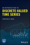
An example of a low counts time series is shown in Figure 1.3, which gives the weekly number of active offshore drilling rigs in Alaska for the period 1990–1997; see Example 2.6.2 for further details. The time series consists of only a few different count values (between 0 and 6). It does not show an obvious trend or seasonal component, so the underlying process appears to be stationary. But it exhibits rather long runs of values that seem to be due to a strong degree of serial dependence. This is in contrast to the time series plotted in Figure 1.4, which concerns the weekly numbers of new infections with Legionnaires' disease in Germany for the period 2002–2008 (see Example 5.1.6). This has clear seasonal variations: a yearly pattern. Another example of a low counts time series with non-stationary behavior is provided by Figure 1.5, where the monthly number of “EA17” countries with stable prices (January 2000 to December 2006 in black, January 2007 to August 2012 in gray) is shown. As discussed in Example 3.3.4, there seems to be a structural change during 2007. If modeling such low counts time series, we need models that not only account for the discreteness of the range, but which are also able to deal with features of this kind. We shall address this topic in Part I of the present book.

All the data examples given above are count time series, which are the most common type of discrete-valued time series. But there is also another important subclass, namely categorical time series, as discussed in Part II of this book. For these, the outcomes stem from a qualitative range consisting of a finite number of categories. The particular case of only two categories is referred to as a binary time series. For the qualitative sleep status data shown in Figure 1.6, the six categories ‘qt’, …, ‘aw’ exhibit at least a natural ordering, so we are concerned with an ordinal time series. In other applications, not even such an inherent ordering exists (nominal time series). Then a time series plot such as the one in Figure 1.6 is no longer possible, and giving a visualization becomes much more demanding. In fact, the analysis and modeling of categorical time series cannot be done with the common textbook approaches, but requires tailor-made solutions; see Part II.

For real-valued processes, autoregressive moving-average (ARMA) models are of central importance. With the (unobservable) innovations¹ being independent and identically distributed (i.i.d.) random variables (white noise; see Example B.1.2 in Appendix B), the observation at time of such an ARMA process is defined as a weighted mean of past observations and innovations,

1.1

In other words, it is explained by a part of its own past as well as by an interaction of selected noise variables. Further details about ARMA models are summarized in Appendix B.3. Although these models themselves can be applied only to particular types of processes (stationary, short memory, and so on), they are at the core of several other models, such as those designed for non-stationary processes or processes with a long memory. In particular, the related generalized autoregressive conditional heteroskedasticity (GARCH) model, with its potential for application to financial time series, has become very popular in recent decades; see Appendix B.4.1 for further details. A comprehensive survey of models within the “ARMA alphabet soup” is provided by Holan et al. (2010). A brief summary and references to introductory textbooks in this field can be found in Appendix B.

In view of their important role in the modeling of real-valued time series, it is quite natural to adapt such ARMA approaches to the case of discrete-valued time series. This has been done both for the case of count data and for the categorical case, and such ARMA-like models serve as the starting point of our discussion in both Parts I and II. In fact, Part I starts with an integer-valued counterpart to the specific case of an AR(1) model, the so-called INAR(1) model, because this simple yet useful model allows us to introduce some general principles for fitting models to a count time series and for checking the model adequacy. Together with the discussion of forecasting count processes, also provided in Chapter 2, we are thus able to transfer the Box–Jenkins method to the count data case. In the context of introducing the INAR(1) model, the typical features of count data are also discussed, and it will become clear why integer-valued counterparts to the ARMA model are required; in other words, why we cannot just use the conventional ARMA recursion (1.1) for the modeling of time series of counts.

ARMA-like models using so-called “thinning operations”, commonly referred to as INARMA models, are presented in Chapter 3. The INAR(1) model also belongs to this class, while Chapter 4 deals with a modification of the ARMA approach related to regression models; the latter are often termed INGARCH models, although this is a somewhat misleading name. More general regression models for count time series, and also hidden-Markov models, are discussed in Chapter 5. As this book is intended to be an introductory textbook on discrete-valued time series, its main focus is on simple models, which nonetheless are quite powerful in real applications. However, references to more elaborate models are also included for further reading.

In Part II of this book, we follow a similar path and first lay the foundations for analyzing categorical time series by introducing appropriate tools, for example for their visualization or the assessment of serial dependence; see Chapter 6. Then we consider diverse models for categorical time series in Chapter 7, namely types of Markov models, a kind of discrete ARMA model, and again regression and hidden-Markov models, but now tailored to categorical outcomes.

So for both count and categorical time series, a variety of models are prepared here to be used in practice. Once a model has been found to be adequate for the given time series data, it can be applied to forecasting future values. The issue of forecasting is considered in several places throughout the book, as it constitutes the most obvious field of application of time series modeling. But in line with the seminal time series book by Box & Jenkins (1970), another application area is also covered here, namely the statistical monitoring of a process; see Part III. Chapter 8 addresses the monitoring of count processes, with the help of so-called control charts, while Chapter 9 presents diverse control charts for categorical processes. The aim of process monitoring (and particularly of control charts) is to detect changes in an (ongoing) process compared to a hypothetical “in-control” model. Initially used in the field of industrial statistics, approaches for process monitoring are nowadays used in areas as diverse as epidemiology and finance.

The book is completed with Appendix A, which is about some common count distributions, Appendix B, which summarizes some basics about stochastic processes and real-valued time series, and with Appendix C, which is on computational aspects (software implementation, datasets) related to this book.