
Chapter 9
Control Charts for Categorical Processes
Having discussed control charts for count processes in the Sections 8.2 and 8.3, we shall now turn to another type of attributes data process ![]() , namely categorical processes, as introduced in Part II. Although now the range (state space)
, namely categorical processes, as introduced in Part II. Although now the range (state space) ![]() of
of ![]() consists of a finite number
consists of a finite number ![]() of (unordered) categories with
of (unordered) categories with ![]() , count values will still play an important role since the most obvious way of evaluating categorical data is by counting the occurrences of categories; see also Chapter 6.
, count values will still play an important role since the most obvious way of evaluating categorical data is by counting the occurrences of categories; see also Chapter 6.
For quality-related applications, ![]() often describes the result of an inspection of an item, which either leads to the classification
often describes the result of an inspection of an item, which either leads to the classification ![]() for an
for an ![]() iff the
iff the ![]() th item was non-conforming of type
th item was non-conforming of type ![]() , or
, or ![]() for a conforming item. A typical example is the one described by Mukhopadhyay (2008), in which a non-conforming ceiling fan cover is classified according to the most predominant type of paint defect, say “poor covering” or “bubbles”. Another field of application is the monitoring of network traffic data with different types of audit events; see Ye et al. (2002) for details. For monitoring such categorical processes, we shall consider two general strategies: if the process evolves too fast to be monitored continuously, then segments are taken from the process at selected times. For each of the resulting samples, a statistic is computed and plotted on a control chart. Here, it is important to carefully consider the serial dependence within the sample; see Section 9.1 for further details. In other cases, it is possible to continuously monitor the process, but then the serial dependence has to be taken into account between the plotted statistics. Control charts for this scenario are presented in Section 9.2. In both cases, we shall first concentrate on the special case of a binary process (that is,
for a conforming item. A typical example is the one described by Mukhopadhyay (2008), in which a non-conforming ceiling fan cover is classified according to the most predominant type of paint defect, say “poor covering” or “bubbles”. Another field of application is the monitoring of network traffic data with different types of audit events; see Ye et al. (2002) for details. For monitoring such categorical processes, we shall consider two general strategies: if the process evolves too fast to be monitored continuously, then segments are taken from the process at selected times. For each of the resulting samples, a statistic is computed and plotted on a control chart. Here, it is important to carefully consider the serial dependence within the sample; see Section 9.1 for further details. In other cases, it is possible to continuously monitor the process, but then the serial dependence has to be taken into account between the plotted statistics. Control charts for this scenario are presented in Section 9.2. In both cases, we shall first concentrate on the special case of a binary process (that is, ![]() ) and then extend our discussion to the general categorical case.
) and then extend our discussion to the general categorical case.
9.1 Sample-based Monitoring of Categorical Processes
In this section, we assume that the categorical process ![]() cannot be monitored continuously. Instead, samples are taken as non-overlapping segments1 from the process at times
cannot be monitored continuously. Instead, samples are taken as non-overlapping segments1 from the process at times ![]() , each being of a certain length
, each being of a certain length ![]() . Note that we restrict ourselves to a constant segment length
. Note that we restrict ourselves to a constant segment length ![]() for simplicity, but at least the Shewhart-type charts could be directly adapted to varying length
for simplicity, but at least the Shewhart-type charts could be directly adapted to varying length ![]() by using varying control limits (Montgomery, 2009, Section 7.3.2). The time distance
by using varying control limits (Montgomery, 2009, Section 7.3.2). The time distance ![]() is assumed to be sufficiently large such that we do not need to worry about the serial dependence between the samples; just the serial dependence within the samples. After having collected the segment, a certain type of sample statistic is computed and then plotted on an appropriately designed control chart.
is assumed to be sufficiently large such that we do not need to worry about the serial dependence between the samples; just the serial dependence within the samples. After having collected the segment, a certain type of sample statistic is computed and then plotted on an appropriately designed control chart.
9.1.1 Sample-based Monitoring: Binary Case
In view of its practical importance, let us first focus on the special case of a binary process ![]() , with the range coded as
, with the range coded as ![]() as in Example 6.3.2. Having available the binary segment
as in Example 6.3.2. Having available the binary segment ![]() , one commonly determines either the sample sum
, one commonly determines either the sample sum ![]() (say, counts of non-conforming items) or the corresponding sample fraction of ‘1’s. Since the sample fraction differs from the count just by a factor
(say, counts of non-conforming items) or the corresponding sample fraction of ‘1’s. Since the sample fraction differs from the count just by a factor ![]() , we shall always consider the resulting count process
, we shall always consider the resulting count process ![]() in the sequel. The original binary process
in the sequel. The original binary process ![]() is now monitored by monitoring this derived count process
is now monitored by monitoring this derived count process ![]() . At this point, the fundamental premise of this section should be remembered: although
. At this point, the fundamental premise of this section should be remembered: although ![]() might exhibit serial dependence, due to taking sufficiently distant segments, we shall assume
might exhibit serial dependence, due to taking sufficiently distant segments, we shall assume ![]() to be serially independent, and hence i.i.d. in its in-control state.
to be serially independent, and hence i.i.d. in its in-control state.
For monitoring ![]() (being i.i.d. in its in-control state), any of the concepts discussed in Chapter 8 can be used, it just has to be adapted to the finite range
(being i.i.d. in its in-control state), any of the concepts discussed in Chapter 8 can be used, it just has to be adapted to the finite range ![]() of
of ![]() . This difference sometimes manifests itself in the name of the resulting control charts. If the counts are plotted directly on a Shewhart-type chart, for instance, it is no longer referred to as a
. This difference sometimes manifests itself in the name of the resulting control charts. If the counts are plotted directly on a Shewhart-type chart, for instance, it is no longer referred to as a ![]() chart, but as an
chart, but as an ![]() chart; see also the discussion in Section 8.2.1, as well as Montgomery (2009). If the sample fractions are plotted, it is called a
chart; see also the discussion in Section 8.2.1, as well as Montgomery (2009). If the sample fractions are plotted, it is called a ![]() chart. Despite this different terminology, the
chart. Despite this different terminology, the ![]() chart still has two control limits
chart still has two control limits ![]() satisfying
satisfying ![]() , which includes the one-sided charts as boundary cases (upper-sided if
, which includes the one-sided charts as boundary cases (upper-sided if ![]() ). Also ARLs are computed as before; see (8.3) and (8.4).
). Also ARLs are computed as before; see (8.3) and (8.4).
Concerning the distribution of the sample counts, the serial dependence structure of the underlying binary process ![]() is of importance. If
is of importance. If ![]() is i.i.d. with
is i.i.d. with ![]() (say, the probability of a non-conforming item), then each sample sum
(say, the probability of a non-conforming item), then each sample sum ![]() is binomially distributed according to
is binomially distributed according to ![]() (Example A.2.1). So the statistics
(Example A.2.1). So the statistics ![]() constitute themselves as an i.i.d. process of binomial counts. But if
constitute themselves as an i.i.d. process of binomial counts. But if ![]() exhibits serial dependence, in contrast, the distribution of
exhibits serial dependence, in contrast, the distribution of ![]() will deviate from a binomial one.
will deviate from a binomial one.
In Deligonul & Mergen (1987), Bhat & Lal (1990) and Weiß (2009f), the case of ![]() being a binary Markov chain with success probability
being a binary Markov chain with success probability ![]() and autocorrelation parameter
and autocorrelation parameter ![]() was considered (Example 7.1.3); that is, with the transition matrix given by (7.6). In this case,
was considered (Example 7.1.3); that is, with the transition matrix given by (7.6). In this case, ![]() follows the so-called Markov binomial distribution
follows the so-called Markov binomial distribution ![]() (which coincides with
(which coincides with ![]() iff
iff ![]() ). While the mean of
). While the mean of ![]() is not affected by the serial dependence, the variance in particular changes (extra-binomial variation if
is not affected by the serial dependence, the variance in particular changes (extra-binomial variation if ![]() , see the discussion in the context of Equation (2.3)):
, see the discussion in the context of Equation (2.3)):

The pmf is given by (Kedem, 1980, Corollary 1.1)

for ![]() (zero inflation if
(zero inflation if ![]() ; see the discussion in Appendix A.2). If the time distance
; see the discussion in Appendix A.2). If the time distance ![]() between successive segments from
between successive segments from ![]() is sufficiently large, the resulting process of counts
is sufficiently large, the resulting process of counts ![]() can still be assumed to be approximately i.i.d. (note that the correlation between
can still be assumed to be approximately i.i.d. (note that the correlation between ![]() and
and ![]() decays exponentially with
decays exponentially with ![]() ), but with a marginal distribution different from a binomial one. This difference in the distribution of
), but with a marginal distribution different from a binomial one. This difference in the distribution of ![]() certainly has to be considered when designing a corresponding control chart (Weiß, 2009f).
certainly has to be considered when designing a corresponding control chart (Weiß, 2009f).
In addition, advanced control schemes, such as the EWMA or CUSUM charts discussed in Section 8.3, can be used for monitoring ![]() . Assuming the counts
. Assuming the counts ![]() to be binomially distributed in their in-control state (that is,
to be binomially distributed in their in-control state (that is, ![]() is assumed to be i.i.d.), Gan (1993) applied the CUSUM scheme described in Section 8.3.1 for process monitoring, while Gan (1990b) used the modified EWMA chart from Section 8.3.3 (with rounding operation as in (8.20)) for this purpose. The application of such an EWMA chart to the case of
is assumed to be i.i.d.), Gan (1993) applied the CUSUM scheme described in Section 8.3.1 for process monitoring, while Gan (1990b) used the modified EWMA chart from Section 8.3.3 (with rounding operation as in (8.20)) for this purpose. The application of such an EWMA chart to the case of ![]() being a binary Markov chain – that is, with
being a binary Markov chain – that is, with ![]() following the Markov binomial distribution – was considered by Weiß (2009f). The computation of ARLs is done in the same way as described in Sections 8.3.1 and 8.3.3, by just using the pmf of the (Markov) binomial distribution. A completely different approach for a sample-based monitoring of an underlying binary Markov chain was recently proposed by Adnaik et al. (2015), who did not compute the sample sums
following the Markov binomial distribution – was considered by Weiß (2009f). The computation of ARLs is done in the same way as described in Sections 8.3.1 and 8.3.3, by just using the pmf of the (Markov) binomial distribution. A completely different approach for a sample-based monitoring of an underlying binary Markov chain was recently proposed by Adnaik et al. (2015), who did not compute the sample sums ![]() as the charting statistics, but instead used some kind of likelihood ratio statistic for each of the successive segments. Finally, Höhle (2010) proposed a log-LR CUSUM chart for monitoring the
as the charting statistics, but instead used some kind of likelihood ratio statistic for each of the successive segments. Finally, Höhle (2010) proposed a log-LR CUSUM chart for monitoring the ![]() under the assumption that these counts follow a marginal (beta-)binomial logit regression model; see Section 7.4.
under the assumption that these counts follow a marginal (beta-)binomial logit regression model; see Section 7.4.
9.1.2 Sample-based Monitoring: Categorical Case
Let us return to the truly categorical case; that is, where the range of ![]() consists of more than two states,
consists of more than two states, ![]() with
with ![]() . As in Section 6.2, we denote the time-invariant marginal probabilities by
. As in Section 6.2, we denote the time-invariant marginal probabilities by ![]() . If the number of different states,
. If the number of different states, ![]() , is small, it would be feasible to monitor the process with
, is small, it would be feasible to monitor the process with ![]() simultaneous binary charts; say, by using the
simultaneous binary charts; say, by using the ![]() -tree method described in Duran & Albin (2009). However, here we shall concentrate on charting procedures in which the information about the process is comprised in a univariate statistic: After having taken a segment from the process, we first compute the resulting frequency distribution as a summary, which then serves as the base for deriving the statistic to be plotted on the control chart. To keep it consistent with the binary case from Section 9.1.1, we concentrate on absolute frequencies:
-tree method described in Duran & Albin (2009). However, here we shall concentrate on charting procedures in which the information about the process is comprised in a univariate statistic: After having taken a segment from the process, we first compute the resulting frequency distribution as a summary, which then serves as the base for deriving the statistic to be plotted on the control chart. To keep it consistent with the binary case from Section 9.1.1, we concentrate on absolute frequencies: ![]() with
with ![]() being the absolute frequency of the state
being the absolute frequency of the state ![]() in the sample
in the sample ![]() , such that
, such that ![]() . With
. With ![]() denoting the binarization of
denoting the binarization of ![]() , we may express
, we may express ![]() .
.
If the underlying categorical process ![]() is even serially independent (so altogether i.i.d.), then the distribution of each
is even serially independent (so altogether i.i.d.), then the distribution of each ![]() is a multinomial one; see Example A.3.3. This case was considered by Marcucci (1985) and Mukhopadhyay (2008), among others, who proposed plotting Pearson's
is a multinomial one; see Example A.3.3. This case was considered by Marcucci (1985) and Mukhopadhyay (2008), among others, who proposed plotting Pearson's ![]() -statistic on a control chart,
-statistic on a control chart,

where ![]() refers to the in-control values of the categorical probabilities. So in the in-control case, the process
refers to the in-control values of the categorical probabilities. So in the in-control case, the process ![]() is i.i.d. with a marginal distribution that might be approximated by a
is i.i.d. with a marginal distribution that might be approximated by a ![]() -distribution (see Horn (1977) concerning the goodness of this approximation). As an alternative, Weiß (2012) proposed using a control statistic that measures the relative change of categorical dispersion. As the underlying categorical dispersion measure, the Gini index (6.1) might be used. If
-distribution (see Horn (1977) concerning the goodness of this approximation). As an alternative, Weiß (2012) proposed using a control statistic that measures the relative change of categorical dispersion. As the underlying categorical dispersion measure, the Gini index (6.1) might be used. If ![]() is i.i.d., following the in-control model, then
is i.i.d., following the in-control model, then

is approximately normally distributed, with a mean of ![]() and variance
and variance ![]() ; see Section 6.2. These approximate distributions for
; see Section 6.2. These approximate distributions for ![]() or
or ![]() may be used during chart design. But since the quality of these approximations is often rather bad (note that
may be used during chart design. But since the quality of these approximations is often rather bad (note that ![]() is often quite small and that the control limit is usually chosen as an extreme quantile), the final design and evaluation of the ARL performance requires simulations in practice.
is often quite small and that the control limit is usually chosen as an extreme quantile), the final design and evaluation of the ARL performance requires simulations in practice.
A sample-based approach is also possible if ![]() is serially dependent. But then, certainly, the distributions of
is serially dependent. But then, certainly, the distributions of ![]() and hence of
and hence of ![]() and
and ![]() will deviate from those given above for the i.i.d. case. If, for instance,
will deviate from those given above for the i.i.d. case. If, for instance, ![]() is an NDARMA process (Section 7.2), then the effect on the distribution can be quantified in terms of the constant
is an NDARMA process (Section 7.2), then the effect on the distribution can be quantified in terms of the constant ![]() from (7.12). Considering the complete vector
from (7.12). Considering the complete vector ![]() , the covariance matrix
, the covariance matrix ![]() from Example A.3.3 is asymptotically inflated by the factor
from Example A.3.3 is asymptotically inflated by the factor ![]() (Weiß, 2013b). For the Gini statistic
(Weiß, 2013b). For the Gini statistic ![]() , variance and mean change (approximately) according to (7.13) and (7.14), respectively, while Weiß (2013b) showed that
, variance and mean change (approximately) according to (7.13) and (7.14), respectively, while Weiß (2013b) showed that ![]() is approximately
is approximately ![]() -distributed.
-distributed.

Figure 9.4 (a)  chart and (b)
  chart applied to simulated sample; see Example 9.1.2.2.
Höhle (2010) proposed a log-LR CUSUM chart if the ![]() stem from a marginal multinomial logit regression model; see Section 7.4.
stem from a marginal multinomial logit regression model; see Section 7.4.
9.2 Continuously Monitoring Categorical Processes
If the process evolves sufficiently slowly, then it is possible to implement a continuous monitoring approach of the categorical process ![]() . So as a new categorical observation
. So as a new categorical observation ![]() arrives, the next control statistic is computed and plotted on the control chart.
arrives, the next control statistic is computed and plotted on the control chart.
9.2.1 Continuous Monitoring: Binary Case
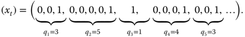
As in Section 9.1.1, let us first focus on the special case of a binary process ![]() . Perhaps the best-known approach for (quasi) continuously monitoring a binary process is by plotting run lengths
. Perhaps the best-known approach for (quasi) continuously monitoring a binary process is by plotting run lengths ![]() on an appropriately designed chart:
on an appropriately designed chart:

As an example,
The monitoring of such runs is a reasonable approach, especially for high-quality processes where ![]() is very small. Small
is very small. Small ![]() implies that long runs are observed, but if
implies that long runs are observed, but if ![]() increases (deterioration of quality), the runs become shorter (and vice versa). So the detection of a decrease in the run lengths is often particularly relevant. Having fixed a truly two-sided design
increases (deterioration of quality), the runs become shorter (and vice versa). So the detection of a decrease in the run lengths is often particularly relevant. Having fixed a truly two-sided design ![]() , we stop monitoring with the
, we stop monitoring with the ![]() th run if either
th run if either ![]() for the first time, or if already
for the first time, or if already ![]() zeros have been observed since the last run (because then,
zeros have been observed since the last run (because then, ![]() will necessarily become larger than
will necessarily become larger than ![]() , but we do not need to wait until the run is finished).
, but we do not need to wait until the run is finished).
Concerning performance evaluation, Remark 9.1.1.1 should be remembered. The ARL – that is, the average number of plotted runs until the first alarm – would be quite misleading, since a single run might comprise a rather large number of original observations. Therefore, the ATS is clearly preferable as a measure of chart performance.
If ![]() is i.i.d. (Bourke, 1991; Xie et al., 2000; Weiß, 2013c), then
is i.i.d. (Bourke, 1991; Xie et al., 2000; Weiß, 2013c), then ![]() is also i.i.d. according to the shifted geometric distribution (Example A.1.5). The ATS can be computed according to (Weiß, 2013c)
is also i.i.d. according to the shifted geometric distribution (Example A.1.5). The ATS can be computed according to (Weiß, 2013c)


Figure 9.5 ATS performance of runs chart against  ; see Example 9.2.1.1.
The monitoring of runs is straightforwardly extended to the Markov case; see Blatterman & Champ (1992) and Lai et al. (2000). The runs ![]() from a binary Markov chain
from a binary Markov chain ![]() according to Example 7.1.3 are still serially independent, but their distribution is no longer shifted geometric. While
according to Example 7.1.3 are still serially independent, but their distribution is no longer shifted geometric. While ![]() has to be treated separately, for
has to be treated separately, for ![]() with
with ![]() , we obviously have
, we obviously have

If ‘1’s are observed more frequently, the runs become quite short on average. In such a case, the CUSUM procedure proposed by Bourke (1991) to monitor the run length in ![]() is more appropriate. This geometric CUSUM control chart is essentially equivalent to the Bernoulli CUSUM control chart, which was proposed by Reynolds & Stoumbos (1999) for an i.i.d. binary process
is more appropriate. This geometric CUSUM control chart is essentially equivalent to the Bernoulli CUSUM control chart, which was proposed by Reynolds & Stoumbos (1999) for an i.i.d. binary process ![]() , and which was extended to the case of a binary Markov chain, as in Example 7.1.3, by Mousavi & Reynolds (2009). These charts are constructed in an analogous way to (8.15): the CUSUM chart is defined by accumulating the contributions to the log-likelihood ratio (log-LR) at times
, and which was extended to the case of a binary Markov chain, as in Example 7.1.3, by Mousavi & Reynolds (2009). These charts are constructed in an analogous way to (8.15): the CUSUM chart is defined by accumulating the contributions to the log-likelihood ratio (log-LR) at times ![]() . The contribution by the
. The contribution by the ![]() th observation equals
th observation equals

where ![]() refers to the relevant out-of-control parameter value of
refers to the relevant out-of-control parameter value of ![]() , while
, while ![]() represents the in-control value. In the Markov case (Example 7.1.3; see also Remark 8.3.2.2),
represents the in-control value. In the Markov case (Example 7.1.3; see also Remark 8.3.2.2), ![]() is computed as before, while
is computed as before, while

An upper-sided CUSUM chart (we restrict to this case, since usually increases in ![]() are to be detected) can now be constructed analogously to (8.13) by defining
are to be detected) can now be constructed analogously to (8.13) by defining
In the i.i.d. case, the CUSUM (9.7) might be rewritten in the form

Note that the plotted statistics of these CUSUM charts go along with the observations, so ![]() . To allow for an exact ARL computation with the MC approach (Section 8.2.2),
. To allow for an exact ARL computation with the MC approach (Section 8.2.2), ![]() can be required to take the form
can be required to take the form ![]() with an
with an ![]() (Reynolds & Stoumbos, 1999); a similar strategy is proposed by Mousavi & Reynolds (2009) for the case of
(Reynolds & Stoumbos, 1999); a similar strategy is proposed by Mousavi & Reynolds (2009) for the case of ![]() being a binary Markov chain. In this case (with
being a binary Markov chain. In this case (with ![]() being a multiple of
being a multiple of ![]() ), the resulting transition matrices
), the resulting transition matrices ![]() for the MC approach are sparse matrices (see Section 8.3.2), since only a few combinations
for the MC approach are sparse matrices (see Section 8.3.2), since only a few combinations ![]() are possible at all for
are possible at all for ![]() . We have
. We have

Note that a lower-sided CUSUM chart can be constructed in an analogous way to (9.8). For a log-LR CUSUM with respect to an underlying logit regression model (Section 7.4), see Höhle (2010).

Figure 9.7 CUSUM charts of Example 9.2.1.2:  against
  .
.
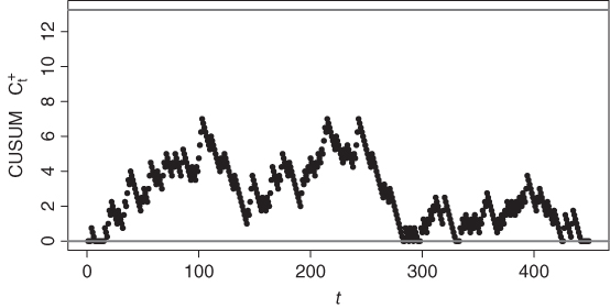
Figure 9.8 CUSUM chart  for fatty liver data; see Example 9.2.1.2.
We conclude by pointing out another approach for continuously monitoring a binary process: the EWMA chart discussed in Section 8.3.3, which was applied to binary processes by Yeh et al. (2008) and Weiß & Atzmüller (2010), among others.
9.2.2 Continuous Monitoring: Categorical Case
Generally, while it is quite natural to check for runs in a binary process, it is more difficult to define a run for the truly categorical case in a reasonable way. One possible solution was discussed in Weiß (2012), where one waits for a segment ![]() of length
of length ![]() , where
, where ![]() is taken from a specified subset
is taken from a specified subset ![]() . But as pointed out in Weiß (2012), waiting times for completely different types of patterns might also be relevant, depending on the actual application scenario. Because of this ambiguity, we shall not further consider the monitoring of runs in a categorical process here.
. But as pointed out in Weiß (2012), waiting times for completely different types of patterns might also be relevant, depending on the actual application scenario. Because of this ambiguity, we shall not further consider the monitoring of runs in a categorical process here.
Instead, we follow the path of Section 9.2.1 and consider CUSUM charts derived from the log-likelihood ratio approach. So let ![]() denote again the in-control value of the marginal distribution
denote again the in-control value of the marginal distribution ![]() , and let
, and let ![]() be the relevant out-of-control value. A CUSUM scheme for the case of an underlying i.i.d. process was proposed by Ryan et al. (2011). In this case, the contribution to the log-LR at time
be the relevant out-of-control value. A CUSUM scheme for the case of an underlying i.i.d. process was proposed by Ryan et al. (2011). In this case, the contribution to the log-LR at time ![]() ,
, ![]() , can be expressed as either
, can be expressed as either

where the latter version uses the binarization ![]() of
of ![]() . The log-LR approach also applies to serially dependent categorical processes. As an example, in analogy to the work by Mousavi & Reynolds (2009) concerning a binary Markov chain (see Section 9.2.1), we consider a categorical Markov chain. Then,
. The log-LR approach also applies to serially dependent categorical processes. As an example, in analogy to the work by Mousavi & Reynolds (2009) concerning a binary Markov chain (see Section 9.2.1), we consider a categorical Markov chain. Then, ![]() is computed as before, where
is computed as before, where

If we are concerned with the particular case of a DAR(1) process as in Examples 7.2.2 and 9.1.2.3, it then follows that

The log-LR-based CUSUM statistic at time ![]() is defined as before, by the recursion
is defined as before, by the recursion
An alarm is triggered once ![]() violates the upper control limit
violates the upper control limit ![]() for the first time. For a log-LR CUSUM with respect to an underlying logit regression model (Section 7.4), see Höhle (2010).
for the first time. For a log-LR CUSUM with respect to an underlying logit regression model (Section 7.4), see Höhle (2010).
An EWMA control chart for the monitoring of a categorical process is proposed by Ye et al. (2002).