3.1 Higher-order INARMA Models

The INAR(1) model, as introduced in Section 2.2, was developed as an integer-valued counterpart to the conventional AR(1) model, mainly by replacing the multiplication in the AR(1) recursion with the binomial thinning operator. This idea is not limited to the first-order autoregressive case, but can also be used to mimic higher-order ARMA models; see Appendix B. The resulting models are then referred to as INARMA models.

While both the INAR(1) and the INMA(1) recursion involve only one thinning operation, the higher-order models need more than one thinning operation at a time. As an example, the counterpart to the full MA(q) model, the INMA(q) model, is defined by a recursion of the form

3.2

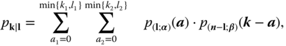
where the thinnings at time are performed independently of each other (in Example 3.1.1, we set ). Here, a time index has been added below the operator “” to emphasize the fact that these are the thinnings being executed at time . Now focussing on one particular innovation, say , it becomes clear that this innovation is altogether involved in thinnings, namely . Since the thinning operations are probabilistic (in contrast to the multiplication used for an MA(q) model), the joint distribution of these thinnings has to be considered – that is, the conditional distribution of given – thereby leading to different types of models of the same model order q.

Until now, a total of four different INMA(q) models have been proposed in the literature, each having slightly different interpretations and probabilistic properties; see Al-Osh & Alzaid (1988), McKenzie (1988), Brännäs & Hall (2001) and Weiß (2008b). To be more precise, the marginal properties are already fixed by definition (3.2), namely:

3.3

where . The joint distributions, however, differ between the different types of INMA(q) processes, as we shall see below. But first, let us look at an example: as for the INAR(1) model (Section 2.2.2), the Poisson distribution plays an important role.

To be able to define different types of INMA(q) models, we follow the approach in Weiß (2008b) and look at the individual counting series. Let be the counting series of the thinning applied to at time for a , with . These might be interpreted as indicators for the individuals being introduced to the considered system at time (“generation ”). If , then the th individual of generation is active at time , where each individual has “lifetime” q.

In view of the general definition (3.2), the -dimensional vectors (each corresponding to one specific individual) have to be i.i.d., but their components might be dependent, thus restricting the activation of an individual during its lifetime. The independence model by McKenzie (1988), for instance, assumes the components of to be mutually independent (so there are no further restrictions concerning the activation of an individual), while the sale model by Brännäs & Hall (2001) requires and defines the vector to be multinomially distributed according to see Example A.3.3. So the sale model assumes that each individual becomes active at most once during its lifetime; an example would be if the “individuals” are perishable goods being produced at day , and they become “active” when they are sold during their shelf-life. Weiß (2008b) analyzed the serial dependence structure of all these INMA(q) models; among other things, he showed that

3.4

So the autocovariance function for different INMA(q) models differs according to the last term. For example, for the independence model by McKenzie (1988), we have , while for the sale model because it is impossible that an individual becomes active twice.

Two types of INAR(p) models have been proposed by Alzaid & Al-Osh (1990) and Du & Li (1991), both being based on the recursion

3.5

where is assumed. Obviously, the conditional distribution of given now has to be specified. Du & Li (1991) assume conditional independence (by analogy to the INMA(q) independence model), while Alzaid & Al-Osh (1990) assume a conditional multinomial distribution (by analogy to the INMA(q) sale model):

see Example A.3.3. Further specialized INAR(p) models can be defined by refining Equation 3.5 by analogy to the INMA(q) case; that is, by considering the counting series of the thinning applied to (“generation ”) at time and by specifying the distribution of .

Let us now look at properties of INAR(p) models. The stationary marginal mean is always given by . For the DL-INAR(p) model, the variance satisfies

3.6

see Silva & Oliveira (2005) for higher-order joint moments. The ACF is obtained from the conventional AR(p) Yule–Walker equations (see (B.13)); that is,

3.7

as shown by Du & Li (1991). For the AA-INAR(p) model, in contrast, Alzaid & Al-Osh (1990) derived an ARMA-like autocorrelation structure, which seems to be the main reason why the DL-INAR(p) model is usually preferred in practice. But there are also reasons why the AA-INAR(p) model is attractive: if having Poisson innovations, its observations are also Poisson distributed and the whole process is time-reversible (Alzaid & Al-Osh, 1990; Schweer, 2015), which is analogous to the Gaussian AR(p) case. The DL-INAR(p) process, in contrast, is time-reversible only in trivial cases (Schweer, 2015), and equidispersed innovations generally do not imply equidispersed observations (Weiß, 2013a). Note that for , (3.6) simplifies to

The conditional mean and variance of the DL-INAR(p) process are given by

3.8

The transition probabilities of the DL-INAR(p) process, which is Markovian of order , can be computed by utilizing the fact that the conditional distribution is a convolution between p binomial distributions and the innovations' distribution (Drost et al., 2009); see (3.12) below for illustration. Mixing and weak dependence properties for the DL-INAR(p) process are discussed by Doukhan et al. (2012 2013) and a frequency-domain analysis is considered by Silva & Oliveira (2005).

In a nutshell, while the INAR(1) model, with its intuitive interpretation and its simple stochastic properties, is very attractive for applications, higher-order extensions are not straightforward. Therefore, in Chapter 4, we discuss an alternative concept for ARMA-like count process models.

To illustrate the potential of some of the extensions mentioned in Remark 3.1.7, let us look at simulated sample paths. The first two parts of Figure 3.4 show paths of non-stationary Poisson INAR(1) processes, where the thinning parameter is kept constant in time, but the innovations' mean varies according to , with representing the covariate information at time (Freeland & McCabe, 2004a). Such trend and seasonality are often observed in practice; corresponding real-data examples are presented in Examples 5.1.6 and 5.1.7. Figure 3.4c shows a sample path with a piecewise pattern, which was generated by a simple SET extension of the Poisson INAR(1) model with one threshold and delay 1; see Monteiro et al. (2012) for further background.

3.2 Alternative Thinning Concepts

The idea behind a thinning operation (and the related time series models) can be modified in diverse ways; see the surveys by Weiß (2008a) and Scotto et al. (2015). Such modified thinning concepts allow for different stochastic properties and alternative interpretation schemes. We shall pick out two of these alternative thinning concepts here, but many further approaches are described in Weiß (2008a) and Scotto et al. (2015).

In view of the BPIs according to Remark 2.1.1.2, the generalized thinning operation, as proposed by Latour (1998), appears reasonable:

3.14

where the random variables (counting series) are allowed to have the full range instead of only . Here, the are required to have mean and variance . Since now the may become larger than 1, the interpretation (2.4) as “survival indicators” is no longer appropriate, but they can be understood as describing a reproduction mechanism: as in Remark 2.1.1.2, might be the number of children being generated by the th individual of the population behind .

Using their generalized thinning operation (which includes binomial thinning as a special case), Latour (1998) extended the INAR(p) model (3.5) by Du & Li (1991) to the GINAR(p) model, which is defined as

3.15

where again is assumed. In (3.15), a time index for the thinning operations is omitted for the sake of readability, but it is understood that all thinnings are performed independently, as in the model by Du & Li (1991).

Although (3.15) has been generalized with respect to (3.5), as well as the Yule–Walker equations (3.7) still hold, while formula (3.6) for the variance has to be modified (Latour, 1998):

3.16

Setting , we would obtain (3.6) again.

A particular instance of generalized thinning, which has received considerable interest in the literature, is the negative binomial thinning operator “” of Ristić et al. (2009), for which the are geometrically distributed with parameter (hence ; see Example A.1.5). Therefore, is conditionally -distributed due to the additivity of the NB distribution (Example A.1.4). Ristić et al. (2009) use this operation to construct a first-order process having a geometric marginal distribution, and refer to it as the new geometric INAR(1) process, abbreviated as NGINAR(1). Also the Poisson INARCH models, discussed later in Section 4.1, might be understood as particular GINAR models using Poisson thinning (Rydberg & Shephard, 2000; Weiß, 2015a).

Another family of thinning operations assumes the counting series to be Bernoulli distributed, but now the thinning probability is allowed to be random itself. The resulting thinning operation is then called random coefficient (RC) thinning, and it has been applied in the context of count time series modeling by a number of authors, including Joe (1996) and Zheng et al. (2007). As a specific instance (Joe, 1996), we consider the case where follows the distribution with ; that is, where and . Then the conditional distribution of given is a beta-binomial distribution (see Example A.2.2), and the thinning operation is referred to as beta-binomial thinning accordingly.

A counterpart to the INAR(1) model from Definition 2.1.1.1 using a general random coefficient thinning operation “” (that is, where the distribution of on is only required to have mean and a certain variance , but is not further specified) was investigated by Zheng et al. (2007). Their RCINAR(1) model is defined by

3.17

While the (conditional) mean and ACF remain as in the INAR(1) case (Section 2.2.1), the effect of the additional uncertainty manifests itself in the (conditional) variance (Zheng et al., 2007):

3.18

Note that is a quadratic function of , and the observations are overdispersed even if the innovations are equidispersed.

Joe (1996) and Sutradhar (2008) considered that instance of the RCINAR(1) model where beta-binomial thinning “” is used. If and if , then the stationary marginal distribution of

3.19

omitting the time index at the thinning operation, is . So innovations and observations are from the same family of distributions, , and have a unique index of dispersion, , both being completely analogous to the case of a Poisson INAR(1) model (Section 2.2.2).

Zheng et al. (2006) extended the RCINAR(1) model to the pth-order RCINAR(p) model, analogous to the INAR(p) model of Du & Li (1991); that is, with thinnings being performed independently (Section 3.1).

3.3 The Binomial AR Model

In many applications, it is known that the observed count data cannot become arbitrarily large; their range has a natural upper bound that can never be exceeded. The models discussed up to now – the INAR(1) model from Definition 2.1.1.1 and all its extensions – can only be applied to count processes having an infinite range . As an example, if we want to guarantee that does not become larger than , then the range of at time would have to be restricted to , which would contradict the innovations' i.i.d. assumption. So different solutions are required for “finite-valued” counts.

One such solution for time series of counts supported on , with a fixed upper limit , is the binomial AR(1) model, which was proposed by McKenzie (1985) together with the INAR(1) model. It replaces the INAR(1)'s innovation term by an additional thinning, , such that this term cannot become larger than .

The condition on guarantees that the derived parameters satisfy ; that is, these parameters can indeed serve as thinning probabilities.

The binomial AR(1) model of Definition 3.3.1 is easy to interpret (Weiß, 2009a). Suppose that we have a system of mutually independent units, each being either in state “1” or state “0”. Let be the number of units being in state “1” at time . Then is the number of units still being in state “1” at time , with individual transition probability (“survival probability”). is the number of units, which moved from state “0” to state “1” at time , with individual transition probability (“revival probability”).

It is known that is a stationary, ergodic and -mixing finite Markov chain (also see Appendix B.2.2). Its marginal distribution is , and the (truly positive) 1-step-ahead transition probabilities are given by

3.21

see McKenzie (1985) and Weiß (2009a). Conditional mean and variance are both linear in , and given by

3.22

Closed-form expressions for the corresponding -step-ahead regression properties are obtained by replacing by (Weiß & Pollett, 2012). Also note that the eigenvalues of the transition matrix according to (3.21) are just given by (Weiß, 2009a). So the speed of convergence of is determined by the value of according to the Perron–Frobenius theorem (Remark B.2.2.1). The ACF of the binomial AR(1) model is of AR(1)-type, given by for (note that might become negative). Closed-form expressions for higher-order joint moments in such a process are provided by Weiß & Kim (2013); the binomial AR(1) process is also time-reversible (McKenzie, 1985).

A pth-order autoregressive version, which uses a probabilistic mixing approach analogous to the CINAR(p) model from Remark 3.1.5 and thus preserves the binomial marginal distribution, was proposed by Weiß (2009b). For the resulting binomial AR(p) model, defined by

3.23

completely analogous to (3.9), the special case of independent thinnings is again relevant. It leads to a pth-order Markov process, the ACF of which satisfies the Yule–Walker equations

3.24

The conditional mean and transition probabilities are given by

3.25

Higher-order (factorial) moments follow in an analogous way to (3.11),

3.26

The binomial AR(1) model and its pth-order extension have a binomial marginal distribution; in particular, their binomial index of dispersion according to (2.3) satisfies . To allow for time-dependent and finite-range counts with (extra-binomial variation), Weiß & Kim (2014) proposed replacing the binomial thinning operations in Definition 3.3.1 (or in (3.23), respectively) by beta-binomial ones (see Section 3.2). The resulting beta-binomial AR(1) model is characterized by the recursion

3.27

where both thinnings use a unique dispersion parameter . Many stochastic properties are analogous to those of the binomial AR(1) model, but the beta-binomial AR(1) model exhibits extra-binomial variation (Weiß & Kim, 2014):

3.28

The transition probabilities are obtained from (3.21) by replacing the involved binomial distributions by beta-binomial ones (Example A.2.2). They can be used to compute the stationary marginal distribution as well as any -step-ahead forecasting distribution exactly as described in Appendix B.2.1, since the beta-binomial AR(1) process is a finite Markov chain. The conditional mean is the same as in (3.22) (thus we also have the same ACF), while the conditional variance is now a quadratic function of (Weiß & Kim, 2014):

3.29

Extensions of the binomial AR(1) model using state-dependent parameters (also see Remark 3.1.7) have been proposed by Weiß & Pollett (2014), for example to describe binomial underdispersion, and by Möller (2016) for SET-type models.

3.4 Multivariate INARMA Models

In many applications, we do not observe a single feature over time, but instead a number of related features simultaneously, thus leading to a multivariate time series. If these multivariate observations are truly real-valued, then, for example, vector autoregressive moving-average (VARMA) models might be appropriate for describing the data; see Appendix B.4.2 for a brief summary. Here, we consider the count data case again; that is, a -variate time series with the range being (or a subset of it). For such multivariate count time series, a number of thinning-based models (designed as counterparts to the VARMA model) have been discussed in the literature; see Section 4 in Scotto et al. (2015) for a survey. These approaches mainly differ in the way of defining a multivariate type of thinning operation. The most widely discussed approach, which is defined in a close analogy to conventional matrix multiplication, is matrix-binomial thinning, which was introduced by Franke & Subba Rao (1993).

Let be a -dimensional count random vector; that is, having the range . Let be a matrix of thinning probabilities. Then Franke & Subba Rao (1993) define the th component of the -dimensional count random vector by

3.31

where the univariate binomial thinning operations (Section 2.2.1) are performed independently of each other. A generalized version of this operator, using univariate generalized thinnings (3.14) instead of binomial ones, was proposed by Latour (1997). We denote this operation by “”, with the th thinning “” satisfying and (for binomial thinning, we have ). It satisfies and

In an analogy to Definition B.4.2.1, a multivariate extension of the INAR(1) model (MINAR(1) model) according to Definition 2.1.1.1 is given by the recursion

3.32

where is an i.i.d. -dimensional count process with finite mean and covariance matrix ; see Franke & Subba Rao (1993), Latour (1997) and Pedeli & Karlis (2013a). Latour (1997) showed that (Condition (B.25) in Appendix B.4.2):

where denotes the identity matrix, still guarantees the existence of a unique stationary solution. The marginal mean is given by , and the autocovariance function is obtained from a slightly modified version of (B.30),

3.33

If the thinning matrix of the MINAR(1) model (3.32) is not a diagonal matrix, then the component processes are generally not univariate INAR(1) processes. Therefore, Pedeli & Karlis (2011 2013b) concentrate on the diagonal case of matrix-binomial thinning (thus also reducing the number of model parameters) such that the cross-correlation between and is solely caused by the innovations. Note that (3.33) simplifies in this case, because becomes :

3.34

where denotes the Kronecker delta. As particular instances of the MINAR(1) model with diagonal-matrix-binomial thinning, they consider the cases with stemming from a multivariate Poisson or negative binomial distribution (Examples A.3.1 and A.3.2). The corresponding component processes then follow the univariate Poisson INAR(1) (Section 2.2.2) or NB-INAR(1) model (Example 2.1.3.3), respectively. Note that Pedeli & Karlis (2011 2013b) use a slightly different parametrization for the MNB distribution from Example A.3.2, with obtained from the relations and for .

Finally, let us turn to the case of multivariate counts having a finite range; that is, a range of the form . At first glance, it appears to be possible to combine Definition 3.3.1 for a binomial AR(1) model with the concept of matrix-binomial thinning (3.31), and to define a model according to the recursive scheme . However, if the matrices are non-diagonal, it may happen that the upper limit is violated, since, for example, might become larger than . So we would have to restrict ourselves to diagonal thinning matrices to ensure the upper limit . But then, due to the absence of an innovations term, the component series would be independent of each other. So, in summary, a non-trivial multivariate binomial AR(1) model using matrix-binomial thinning is not possible.

For this reason, restricting to the bivariate case, Scotto et al. (2014) introduced another type of thinning operation, based on the bivariate binomial distribution of Type II (Example A.3.5). Let be a bivariate count random variable with range . The bivariate binomial thinning operation “” is defined by requiring the conditional distribution

3.35

where the thinning parameter has to satisfy the restrictions given in Example A.3.5. Note that in contrast to matrix-binomial thinning, bivariate binomial thinning (3.35) generates cross-correlation (if ) and preserves the upper bound at the same time. Furthermore, the marginals of just correspond to univariate binomial thinnings: .

Using this operation, Scotto et al. (2014) defined the bivariate binomial AR(1) model with upper limit by extending Definition 3.3.1 as follows: let for be separate sets of parameters according to Definition 3.3.1, derive accordingly. Choose such that and become valid BVB-parameters. Then the -AR(1) process is defined by the recursion

3.36

where the thinnings are again performed independently of each other. By construction, the components of this process are just univariate binomial AR(1) processes with parameters and , respectively, and these components are cross-correlated to each other (Scotto et al., 2014):

3.37

To numerically compute these and further properties of the model, it should be noted that constitutes a finite Markov chain (so (B.4) holds) with transition probabilities

3.38

where abbreviates the pmf of the distribution as given in Example A.3.5. Note that is even a primitive Markov chain and hence -mixing with a uniquely determined stationary marginal distribution. Further properties and a data example are provided by Scotto et al. (2014).