7.1 Parsimoniously Parametrized Markov Models

Perhaps the most obvious approach to model a categorical process with state space is to use a (homogeneous) pth-order Markov model; see (B.1) for the definition:

The idea of having a limited memory is often plausible in practice, and the Markov assumption is also advantageous, say for parameter estimation (see Remark B.2.1.2) or for forecasting. Concerning the latter application, it is important to note that a pth-order Markov process can always be transformed into a first-order one (for , we speak of a Markov chain; see Appendix B.2) by considering the vector-valued process with . And for a Markov chain with transition matrix , in turn, -step-ahead transition probabilities are obtained as the entries of the matrix . So, to summarize, -step-ahead conditional distributions of the form are calculated with relatively little effort for a pth-order Markov process.

Then, point forecasts are computed as a mode of this conditional distribution, or, for an ordinal process, as the median. In the ordinal case, it is obvious how to define a prediction region on level : for a two-sided region, the limits are defined based on the - and the -quantile of the conditional distribution, while one uses the - or -quantile, respectively, in case of a one-sided region (“best/worst-case scenario”). If is very small, however, it may be that one ends up with a trivial region (say, the full range ). The same problem may occur in the nominal case, but here, in addition, a reasonable definition of a prediction region is more difficult because of the lack of a natural ordering. Commonly, one defines a prediction set for to consist of the most frequent states in (most frequent with respect to the -step-ahead conditional distribution) such that the required level is ensured.

The computation of the serial dependence measures (6.3), (6.4) for a Markov chain with transition matrix and stationary marginal distribution , as in Example 7.1.1, is done by first computing the matrices of bivariate joint probabilities via .

While a full Markov model might be a feasible approach if p is very small, higher orders p will cause a practical problem: a general pth-order Markov process (that is, where the conditional probabilities are not further restricted by parametric assumptions) has a huge number of model parameters, , which increases exponentially in p. This problem becomes visible in Figure 7.3, where the possible paths in the past for increasing p are illustrated. Each path (out of such paths) requires parameters to be specified to obtain the conditional distribution , thus leading to altogether parameters. For the EEG sleep state data from Example 6.1.1, for instance, we have states such that a first-order Markov model would already require 30 parameters to be estimated (from only observations available).

To make Markov models more useful in practice, the number of parameters has to be reduced. One suggestion in this direction is due to Bühlmann & Wyner (1999): the variable-length Markov model (VLMM). Here, the “embedding Markov model” possibly has a rather large order p, but then several branches of the tree in Figure 7.3 are “cut” by assuming identical conditional distributions; that is, by assuming shortened tuples with such that

7.1

for all and all . Hence, if the last observations have been equal to , the remaining past is negligible. So the order of the embedding Markov model determines the maximal length of the required memory, but depending on the observed past, a shorter memory may also suffice, which explains the name “variable-length” Markov model. While this kind of parameter reduction is reasonable at a first glance, the number of possible VLMMs is very large, so the model choice is non-trivial. Algorithms for constructing VLMMs have been proposed by Ron et al. (1996).

Another proposal to reduce the number of parameters of the full Markov model aims at introducing parametric relations between the conditional probabilities: the pth-order mixture transition distribution (MTD(p)) model of Raftery (1985). The idea is to start with a (full) Markov chain with transition matrix (Appendix B.2), and to define the pth-order conditional probabilities as a mixture of these transition probabilities:

7.2

Here, is required. A common further restriction is to assume all , but it would even be possible to allow some to be negative (Raftery, 1985).

While the general pth-order Markov model has parameters, this number is now reduced to ; that is, we have the number of parameters for a Markov chain (the ones from ) plus only one additional parameter for each increment of p. Since the conditional probabilities are just some kind of weighted mean of transition probabilities from , Raftery (1985) showed that the stationary marginal distribution for positive is simply obtained as the solution of

7.3

see also (B.4). Furthermore, Raftery (1985) showed that the bivariate probabilities satisfy a set of Yule–Walker-type equations. Denoting for , and , then

7.4

For , for instance, we immediately obtain that , and the remaining s are computed via (7.4). In this way, (7.4) can be used to compute serial dependence measures such as Cramer's from (6.3) or Cohen's from (6.4), although simple closed-form results will usually not be available due to the general form of . Note that because of (7.3), Equation 7.4 can also be rewritten in a centered version as

Approaches for parameter estimation are discussed by Raftery & Tavaré (1994). For a survey of results for MTD models, see Berchtold & Raftery (2001).

A further reduction in the number of parameters is obtained by assuming parametric relations for . Jacobs & Lewis (1978c) and Pegram (1980) suggest defining with such that

7.5

Jacobs & Lewis (1978c) require and refer to these models as the discrete autoregressive models of order p (DAR(p)), while Pegram (1980) even allows some to be negative (see above). This model has only parameters. We shall provide a more detailed discussion of it in Section 7.2 when considering the extension to a full discrete ARMA model. Also, the discussion of another type of parsimoniously parametrized Markov model, namely the autoregressive logit model, is postponed until later; see Example 7.4.4.

With increasing p, not only the number of parameters of a binary Markov model increases rapidly (); in general, we also do not have an AR(p)-like autocorrelation structure anymore. An exception is the binary version of the MTD(p) model. If is assumed to be parametrized as in (7.6) – that is, – then it immediately follows that (7.5) holds. This implies an AR(p)-like autocorrelation structure; see Section 7.2 below.

A closely related approach to the binary MTD(p) and DAR(p) models is the binary AR(p) model of Kanter (1975), which was extended to a full binary ARMA(p, q) model by McKenzie (1981) and Weiß (2009d). The model recursion looks somewhat artificial, as it uses addition modulo 2. On the other hand, this definition also allows for negative autocorrelations; see the cited references for further details.

7.2 Discrete ARMA Models

Based on preliminary works (Jacobs & Lewis, 1978a–1978c) on discrete counterparts to the ARMA(1, q) and AR(p) model, respectively, Jacobs & Lewis (1983) introduced two types of discrete counterparts to the full ARMA(p, q) model. In particular the second of these models, referred to as the NDARMA model by Jacobs & Lewis (1983), is quite attractive, since its definition and serial dependence structure are very close to those of a conventional ARMA model; see also our discussion of the count data version of this model in Section 5.3. Let us pick up Definition 5.3.1 and adapt it to the categorical case (Weiß & Göb, 2008).

Note that the NDARMA(p, q) model has only parameters. Although its recursion is written down in an “ARMA” style, does nothing but choose the state of either or … or . So is generated as a random choice from (a random mixture). But as we shall see in (7.9), the ARMA-like notation is indeed adequate and reasonable for NDARMA processes.

With the same argument as in Section 5.3, it follows that and have the same stationary marginal distribution; that is, for all . It is useful to know that an NDARMA model can always be represented by a -dimensional finite Markov chain with a primitive transition matrix (Jacobs & Lewis, 1983; Weiß, 2013b). Using this Markov representation, Weiß (2013b) showed that an NDARMA process is -mixing with exponentially decreasing weights (see Definition B.1.5) such that the central limit theorem (CLT) in Billingsley (1999, p. 200) is applicable. Conditional distributions of an NDARMA process are determined by

7.8

which reduces to an expression like the one in (7.5) for the DAR(p) case (). Only in the latter case, we have Markov dependence (of order p), while an NDARMA(p, q) process with is not Markovian, although it can be represented as a -dimensional Markov chain.

Let us now investigate the serial dependence structure of an NDARMA(p, q) process using the concepts described in Section 6.3. Only positive dependence is possible (implying that NDARMA processes tend to show long runs of their states); that is, , and it even holds that (Weiß & Göb, 2008). These properties can be utilized to identify if an NDARMA model might be appropriate for a set of time series data (by looking at the sample versions ). For example, the serial dependence measures for the wood pewee time series shown in Figure 6.4 clearly deviate from NDARMA behavior, with negative dependencies and strong deviation between and .

Since both measures lead to identical results anyway, let us focus on in the following. itself is obtained from a set of Yule–Walker-type equations (Weiß & Göb, 2008):

7.9

where the satisfy

which implies for , and . Note the analogy to (5.22) for the autocorrelation function in the count data case. The relation between and the bivariate distributions with lag is given by

7.10

see Weiß & Göb (2008). The equations (7.9) can now be applied in an analogous way to the use of the original Yule–Walker equations for an ARMA process; see Appendix B.3. For a DMA(q) model (), we have . Hence, such that vanishes after lag ; see (B.11) for the corresponding MA(q) result. So the model order q can be estimated using or , as described in Appendix B.3.

For a DAR(p) model (), in turn, we have , which corresponds exactly to the AR(p) result (B.13). Hence, defining the partial Cohen's (or partial Cramer's ) with exactly the same relation as in Theorem B.3.4 (just replacing by or ), we obtain a tool for identifying the autoregressive order p: for lags . These results also apply to the binary MTD(p) model; see Section 7.1, which was shown to have an DAR(p) dependence structure, and where according to Example 6.3.1.

Now let us look at the sample measures of dispersion from Section 6.2 and the sample measures of serial dependence from Section 6.3. There, we presented the asymptotic properties of these measures if applied to i.i.d. categorical processes. Now let us analyze what changes if these measures are applied to an underlying NDARMA process.

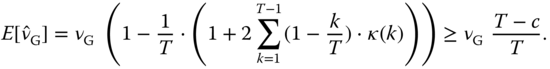
The asymptotic results for the Gini index (6.1) and the entropy (6.2) are easily adapted. As shown by Weiß (2013b), they are still asymptotically normally distributed, and the i.i.d. variance just has to be inflated by the factor

7.12

While in the i.i.d. case, it is given by for a DAR(1) model, as an example. So altogether, we have

7.13

At least for the sample Gini index, an exact bias correction is possible. As shown by Weiß (2013b),

7.14

The latter formula provides a simple way to obtain an approximate bias correction, and it is exact in the i.i.d. case.

For the sample serial dependence measures from Section 6.3, asymptotic normality can also be established, and explicit expressions for the asymptotic variances can be derived. But these expressions are much more complex than in the i.i.d. case, so we refer the reader to Weiß (2013b) for further details.

Let us now look at applications of discrete ARMA models. An application of count time series to video traffic count data was sketched in Example 5.3.2. For categorical time series, Chang et al. (1984) and Delleur et al. (1989) used discrete ARMA models for modeling daily precipitation. While Chang et al. (1984) used a three-state model (that is, ) representing either dry days, days with medium or with strong precipitation, Delleur et al. (1989) used a two-state model (that is, ) to just distinguish between wet and dry days. If the rainfall quantity also has to be considered, Delleur et al. (1989) propose using a state-dependent exponential distribution, analogous to the corresponding approach with HMMs (Sections 5.2 and 7.3). Another field of application of discrete ARMA models is DNA sequence data; see, for example, Dehnert et al. (2003). Returning to this application, let us consider the DNA sequence corresponding to the bovine leukemia virus.

7.3 Hidden-Markov Models

Another important type of model for categorical processes with a non-Markovian serial dependence structure is the hidden-Markov model (HMM), which we are already familiar with from the count data case; see Section 5.2 as well as the book by Zucchini & MacDonald (2009) and the survey article by Ephraim & Merhav (2002). HMMs refer to a bivariate process , in which the hidden states (latent states) constitute a homogeneous Markov chain (Appendix B.2) with range and , and where the observable random variables (now also categorical with state space ) are generated conditionally independently, given the state process; see Figure 5.7 for an illustration of the data-generating mechanism.

As mentioned in Section 5.2, we may interpret a HMM as a “probabilistic function of a Markov chain” (Baum & Petrie (1966); see also Remark 7.3.3). While we shall again concentrate on HMMs for stationary processes, these models can also be used for non-stationary processes by, for example, including covariate information (Remark 5.2.6). HMMs for categorical processes have been applied in many contexts: in biological sequence analysis (Churchill, 1989; Krogh et al., 1994) and especially in fields related to natural languages:

• speech recognition (Rabiner, 1989): transforming spoken into written text
• text recognition (Makhoul et al., 1994; Natarajan et al., 2001): handwriting recognition or optical character recognition
• part-of-speech tagging (Cutting et al., 1992; Thede & Harper, 1999): where each word in a text is assigned its correct part of speech.

As described in Section 5.2, an HMM for is defined based on three assumptions:

• the observation equation (5.8):
• the state equation (5.9):
• the Markov assumption with state transition probabilities (5.11):

As before, we denote the hidden states' transition matrix by . The initial distribution of is assumed to be determined by the stationarity assumption; that is, , where satisfies the invariance equation (see (B.4)). In contrast to Section 5.2, the time-homogeneous state-dependent distributions – that is, for all – are categorical distributions, each having parameters. So altogether, we have parameters for the hidden states, plus parameters related to the observations.

Most of the stochastic properties discussed in Section 5.2 directly carry over to the categorical case (certainly except those referring to moments, since the latter do not exist for categorical random variables). For instance, defining again the diagonal matrices for , the marginal pmf and the bivariate probabilities are given by (5.13); that is, by

7.15

Furthermore, maximum likelihood (ML) estimation is still possible, as described in Remark 5.2.3, the forecast distributions (5.19) and (5.20) remain valid, and both decoding schemes from Remark 5.2.4 are also applicable in the categorical case.

As the main difference, the serial dependence structure of the HMM's observations can no longer be described in terms of the ACF, and measures such as Cramer's (6.3) or Cohen's (6.4) have to be computed using (7.15). Measures of categorical dispersion (Section 6.2), such as the Gini index (6.1) or entropy (6.2), are also available in this way.

Picking up Remark 7.2.3, it is obvious by model construction that any binarization of the HMM's observation process , with for a , follows an HMM again, now with state-dependent probabilities and . For such a binary HMM, in turn, moments and hence the ACF will be well-defined, where the relationship between ACF and has already been investigated; see Example 6.3.2.

7.4 Regression Models

In Section 5.1, we introduced regression models for time series of counts, the main advantage of which is their ability to easily incorporate covariate information, the latter being represented by the (possibly deterministic) vector-valued covariate process . In our discussion, we focussed on generalized linear models (GLMs), where the observations’ conditional mean is linked to a linear expression of the “available information”. The available information is not necessarily limited to the covariate information, but it may also include past observations of the process, as in the case of the conditional regression models according to Definition 5.1.1. If, however, only the current covariate is required for “explaining” the current observation, then we referred to such a situation as a marginal regression model (5.5) (Fahrmeir & Tutz, 2001). In the sequel, we shall see that the regression approach can also be adapted to the case of the observations process being categorical. A much more detailed discussion of such categorical regression models together with several real-data examples is provided in Chapters 2 and 3 of the book by Kedem & Fokianos (2002).

Before turning to the general categorical case, let us first look at the special situation, where is a binary process with the state space being coded as (see Example 6.3.2); that is, where the are Bernoulli random variables (Example A.2.1). The parameter of the Bernoulli distribution is its “success probability”, which is also equal to its mean. Hence, it lends itself to proceed in the same way as in Section 5.1; that is, to define a GLM with respect to this mean parameter. So Definition 5.1.1 now reads as follows.

The definition (5.5) of a marginal regression model is adapted accordingly. Note that is expressed equivalently as ; this allows for a simplified notation of the (partial) likelihood function (Remark 5.1.5), since now equals . A detailed discussion of likelihood estimation for binary regression models is provided by Slud & Kedem (1994).

While in the count data case, we had to ensure that always produces a positive value, here, we even have to ensure that the value of is in the interval . If one wants to avoid severe restrictions concerning the parameter range for , it is recommended to use response functions with range ; for example, a (strictly monotonic increasing) cdf. The most common choice is the cdf of the standard logistic distribution, leading to a logit model.

Possible alternatives to the logit approach are the probit model (based on the cdf of the standard normal distribution), the log–log model (cdf of standard maximum extreme value distribution), or the complementary log–log model (cdf of standard minimum extreme value distribution); see Section 2.2 in Kedem & Fokianos (2002) for further details.

To extend the methods described before to the general categorical case – that is, where has the state space – it is helpful to look at the binarization of , defined by if , with being the unit vectors (see Example A.3.3). If is distributed according to (unit simplex, see Remark A.3.4), then is multinomially distributed according to , and its th component follows the Bernoulli distribution . The basic idea in the sequel is to apply the above binary approaches (especially the logit approach) to these components .

Because of the sum constraint , it is reasonable to concentrate on the reduced vectors (then ), the distribution of which is denoted by according to Example A.3.3. To further simplify the notation, we define the open -part unit simplex

then satisfies , and we just write .

Following Fahrmeir & Kaufmann (1987), Kedem & Fokianos (2002) and Fokianos & Kedem (2003), we now extend Definition 7.4.1 to a conditional categorical regression model.

Analogous to the binary case, the probabilities are expressed in a simple way, namely as (the component of expresses ). These probabilities are required for (partial) likelihood computation. Likelihood estimation for categorical regression models is discussed by Fahrmeir & Kaufmann (1987) and Fokianos & Kedem (2003) as well as in the book by Kedem & Fokianos (2002).

To illustrate Definition 7.4.3, let us consider a particular instance of a categorical GLM: the categorical logit model as discussed by Kedem & Fokianos (2002) and Fokianos & Kedem (2003).

A particular example of the categorical logit model described in Example 7.4.4 is a th-order autoregressive model (analogous to (7.16); see also Kedem & Fokianos (2002) and Fokianos & Kedem (2003)), where is composed of ; that is, of dimension . Hence, the total number of model parameters is given by , with the components’ parameter vectors being of dimension . So the th-order autoregressive logit model can be understood as a parsimoniously parametrized th-order Markov model; see also Section 7.1. Partitioning the components of as with the consisting of parameters, we can rewrite the autoregressive logit model’s recursion as

7.19

A non-Markovian categorical regression model with an additional feedback component, analogous to equation (7.17), was developed by Moysiadis & Fokianos (2014).

We conclude this section by pointing out that the regression approach can also be used for ordinal time series; see Kedem & Fokianos (2002) and Fokianos & Kedem (2003). To simplify the presentation, we first discuss a marginal regression model, but the model is easily extended to a conditional regression model.

The ordinal regression approach of Example 7.4.6 is easily modified to obtain an autoregressive model. As for model (7.19), we skip one component of the binarization of . But in view of the thresholds (7.20), this time, it is advantageous to define following (Example A.3.3). Combining approaches (7.19) and (7.22), we define an ordinal autoregressive logit model as (Fokianos & Kedem, 2003):

7.23

Note that the -dimensional parameter vectors do not depend on (certainly, this would also be possible), so that the model has only parameters.

For further information on ordinal regression models, consult Kedem & Fokianos (2002) and Fokianos & Kedem (2003).