4.1 Poisson Autoregression

Due to the multiplication problem discussed in Section 2.1 , the ARMA models of Definition B.3.5 are not applicable to the count data case. The models presented in Chapters 2 and 3 circumvented this problem by replacing the multiplications with a type of thinning operation, that ensures that these modified model recursions always produce integer values. The INGARCH models to be presented in this chapter use another solution to the multiplication problem: a linear regression of the conditional means . To construct an AR(1)-like model, for instance, the AR(1) recursion is transferred to the level of conditional means as . Then the count at time is generated by using, say, a conditional Poisson distribution – that is, – thus guaranteeing that the outcomes are always integer values. This approach is not only related to linear regression; it also shares analogies with the definition of an ARCH(1) model (Definition B.4.1.1 ), where the autoregression is defined at the level of conditional variances: . Such ARCH models are extended beyond pure autoregression by also including past conditional variances in the model recursion; see the GARCH equation (B.20). For example, the GARCH() model is determined by . Picking up this idea, an INGARCH() model is defined by also including a feedback term, now with respect to the previous conditional mean: .

The full INGARCH model was introduced by Rydberg & Shephard (2000), Heinen (2003) and Ferland et al. (2006). The name indicates that, as mentioned before, this model can be understood as an integer-valued counterpart to the conventional GARCH model, but also see the discussion in Remark 4.1.2 below. Conditioned on the past observations, the INGARCH model assumes an ARMA-like recursion for the conditional mean. Depending on the choice of the conditional distribution family, different INGARCH models are obtained. The basic INGARCH model, which is discussed in this section, assumes a conditional Poisson distribution.

If , the model of Definition 4.1.1 is referred to as the INARCH(p) model.

Although having the equidispersed Poisson distribution as a conditional distribution, the INGARCH model is well suited for overdispersed counts, since it satisfies

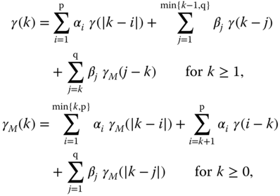
provided that these moments exist. In fact, Ferland et al. (2006) showed that for , the INGARCH process exists and is strictly stationary, with finite first- and second-order moments. In this case, the mean equals

4.1

and variance and autocovariances are determined by a set of Yule–Walker-like equations (Weiß, 2009c):

4.2

where and . Note the analogy to equations (B.18) for the conventional ARMA model (Appendix B.3 ), and note the difference to the ARCH case (Appendix B.4.1 ), where the non-squared observations are uncorrelated.

Further results concerning likelihood estimation, especially on the asymptotic properties of the resulting ML estimators, are provided by Ferland et al. (2006), Fokianos et al. (2009) and Cui & Wu (2016).

It should be mentioned that the slow decay of the SACF of the transactions counts from Example 4.1.5 is not necessarily caused by a long memory, but might also be explained by, for example, change points in the process (Kirch & Kamgaing, 2016, 10.5.2.1). Generally, it is well known that transactions data often exhibit an intraday pattern because of higher trading activity at the beginning and at the end of a trading day; see, for example, Wood et al. (1985). But here, for illustration, we continue with the INGARCH(1, 1) modeling.

An important subfamily of the INGARCH models from Definition 4.1.1 is the class of purely autoregressive (Poisson) INARCH(p) models, where and

4.3

Such INARCH models were discussed by Rydberg & Shephard (2000) and Weiß (2009c) in some detail. The INARCH(p) model constitutes a pth-order Markov model, thus being a competitor to the DL-INAR(p) model (3.5). The Poisson INARCH(p) model can also be understood as a particular GINAR(p) model, see the discussion in Section 3.2 . It has simple Poisson transition probabilities,

4.4

which is attractive for CML estimation according to (B.6). It also has a linear conditional mean and variance, both given by (also see (3.8) for the DL-INAR(p) model). In particular, equations (4.2) simplify to

4.5

that is, we have the typical AR(p) autocorrelation structure (see (B.13)). As a consequence, the model order p can be identified by inspecting the (S)PACF.

Comparing with the discussion in Section 3.1 , it becomes obvious that the INGARCH approach is easier to use when handling a higher-order ARMA-like autocorrelation structure than the INARMA approach; see also Remark 4.1.3. On the other hand, closed-form expressions for the stationary marginal distribution or for -step ahead forecasting distributions are difficult to find, even in the simplest case of an INARCH(1) model.

While the 1-step-ahead conditional properties of the INARCH(1) model are very simple, there is no closed-form formula for the stationary marginal distribution, or for the -step-ahead conditional properties with . To obtain these, at least numerically, the MC approximation of Remarks 2.1.3.4 and 2.6.3 has to be adopted.

4.2 Further Types of INGARCH Models

The standard INGARCH model with its conditional Poisson distribution exhibits unconditional overdispersion, but the degree of overdispersion is determined by the actual autocorrelation structure (say, for the Poisson INARCH(1) model from Example 4.1.6). As a consequence, this model was not able to describe the strong volatility of the transactions counts in Example 4.1.5. To overcome this limitation, Xu et al. (2012) proposed the family of dispersed INARCH models (DINARCH), which again assume a linear relationship for the conditional mean (see (4.3)), but include an additional (constant) scaling factor for the conditional variance:

4.7

So the characteristic feature is a time-invariant conditional dispersion index, being equal to . Obviously, the Poisson INARCH model is an instance of the DINARCH model with .

For the case (see Example 4.1.6), the unconditional mean and variance are given by

4.8

that is, allows control of the (unconditional) degree of dispersion independently of (Xu et al., 2012).

A brief overview of the different INGARCH models is provided in Table 4.3.

Model	Conditional distribution	Conditional dispersion index
Poi. INGARCH		1
NBXu-INGARCH	with
NBZhu-INGARCH	with
GP-INGARCH	with
ZIP-INGARCH	with

Both types of NB-INGARCH model (as well as the GP-INGARCH model to be discussed in the next example) are instances of the CP-INGARCH model (see Example A.1.2 about the compound Poisson distribution) introduced by Gonçalves et al. (2015). It is given by

4.9

where denotes the pgf of the compounding distribution (assumed to be normalized to for uniqueness), which is generally allowed to depend on time through past observations. If is constant in time, then the above condition still guarantees the existence of a strictly stationary and ergodic solution for the CP-INGARCH model, having finite first- and second-order moments (Gonçalves et al., 2015). Further restricting to the case , the resulting CP-INARCH model becomes an instance of the DINARCH model, where .

Note that Zhu (2012a) also allows to become negative (conditional underdispersion), but this case has to be considered with caution in view of the problems discussed below (Example A.1.6 ).

The INGARCH approach also allows generation of zero inflation.

Finally, let us have a look at the case of counts having the finite range with some fixed upper limit (see also the discussion in Section 3.3). None of the above models can be used in such a situation, since the respective conditional distribution has an unbounded range.

As for the other INARCH(1) models, there are no closed-form expressions available for the stationary marginal distribution or the -step-ahead conditional distributions with . But due to the finite range, and in complete analogy to the case of the beta-binomial AR(1) model (see the discussion in Section 3.3), these can be exactly computed numerically by utilizing the Markov property; see Appendix B.2.1 for details.