CHAPTER 4
Little’s Law
What is the reason that we reduce inventory? It is to make the finances easier.
For example, what if 500,000,000 yen of work in process and inventory was reduced and this 500,000,000 yen was in the accountant’s safe? The accountant could invest this money … and we could make a profit of several percent from this … But when this money is on the gemba in the form of materials, we now have to borrow money.
Little’s Law links the throughput rate, inventory, and flow time (i.e., the time a specific unit needs to flow through the process). It explains that for a given throughput rate, a manager can only decrease the amount of time it takes for a unit to go through the process from the start to the end by decreasing the inventory level. Also, without a decrease in the inventory level, average flow time can only be reduced by increasing the throughput rate, that is, capacity.
All processes that are stable—that is, the input rate equals the output rate in the long term—can best be described using the three measures identified in Little’s Law. These are the work-in-process (WIP) inventory, the throughput rate, and the process flow time. The WIP is the inventory within the process.
For example, if you were in charge of cooking hamburgers, the throughput rate of the hamburger cooking process would be the rate at which hamburgers would be completed by the process. So if you prepare 1 hamburger every 15 minutes, the throughput rate for completed hamburgers would be 1 hamburger every 10 minutes or 6 hamburgers/hour. The process flow time is the total time from the start of processing of an item to the completion of the same item. To cook hamburgers you measure the flow time starting from the time you take the beef from the refrigerator until you place the top of the bun onto the hamburger and place this sandwich onto the plate. While the hamburger is being made, it is considered WIP inventory. The amount of WIP would be measured by counting the number of hamburgers within the process.
When the process is stable, the relationship between the average WIP inventory, the average throughput rate, and the average flow time is given by Little’s Law as shown in Equation 4.1. The average amount of WIP inventory in the line (I) is directly proportional to the product of the average throughput rate (R) multiplied by the average flow time (T).
|
(4.1) |
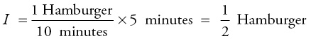
If we know two of the three variables in Little’s Law, we can calculate the third variable. For example, in the hamburger example, if the throughput rate is 1 hamburger every 10 minutes and if the process flow time is 5 minutes (i.e., the time from the hamburger starting as a raw beef hamburger patty until it is a perfectly cooked medium rare hamburger placed in a prepared bun on a plate), then the WIP inventory (I) is calculated as:
This example is interesting because it implies that the process is actually idle 50 percent of the time. So if we measured the inventory instead of calculating it, we might count the number of hamburgers in process every 5 minutes. If we did this we might get data similar to that in Table 4.1.
In this example, we counted the number of hamburgers at eight different times, and there was 1 hamburger in the process four of the times and no hamburgers the other four times, so there was an average of 0.5 hamburgers.
But who cares about hamburgers!!
A more interesting problem that occurs to all of us on a daily basis is how long we have to stand in line to place an order at Starbucks. When we are desperate for a cup of coffee in the morning, a wait can seem interminable!! For example, you are at the back of the line at Starbucks, and there are eight people in line in front of you. You observe that people are being served at the rate of 1 customer/minute. Quickly calculating that the time until you order your own coffee (i.e., your flow time in the line) is equal to the number in line (the WIP inventory, I ) (8 customers in front of you) divided by the throughput rate as:
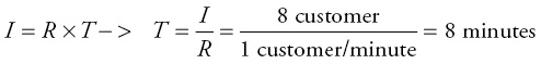
Table 4.1 Observed inventory (hamburger) in process
| Time | Number of hamburgers |
| 0 | 1 |
| 5 | 1 |
| 10 | 0 |
| 15 | 0 |
| 20 | 1 |
| 25 | 1 |
| 30 | 0 |
| 35 | 0 |
| Average | 4/8 = 0.5 |
Imagine a common service system. The customer arrives, stands in line to wait for their turn, and then is served by whatever the service process is. When customers or items have to wait for processing or for service, the first activity is to stand in line. The second activity is the actual service process. It is important not to combine them. They happen separately from each other and need to be distinctly shown. In the example in Figure 4.1, the manager measured either the number waiting to be served or the time to do the activity. The manager then calculated the third variable for that activity. The calculated variable is underlined in the flow diagram in Figure 4.1 for ease of reference. The first activity was to stand in line. The manager measured the average line as 1 customer being the observed throughput rate 0.5 customer/minute. The waiting time can then be calculated as:
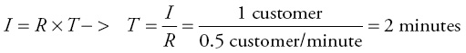
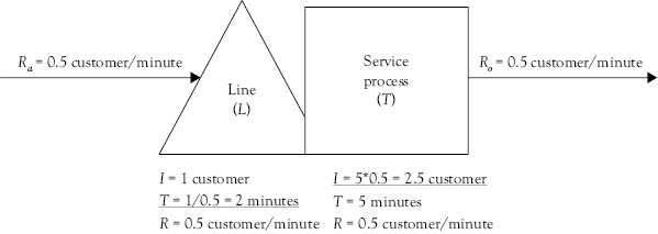
Figure 4.1 Flow diagram of “stand in line” activity
A flow chart for the Eis-Sahne Ice Cream shop, with the times of the activities entered, is shown in Figure 4.1. The manager of the shop measured the average arrival and departure rate at the shop and found that 1 customer arrived every 5 minutes (Ra = 1 customer/5 minutes). Over the long run (e.g., 2 hours) both the arrival rate and departure rate were the same (i.e., Ra = Ro), so the process was stable. For the second activity, “ Customer Places Order,” the manager measured the amount of time to do this as 0.5 minute and calculated the number of people in service as 0.1 customer (I = 0.5 * 1/5 = 0.1 customer), which is underlined in the flow diagram in Figure 4.2. All the activities in the Eis-Sahne process are shown in Figure 4.2, and for each activity, the measured data was entered. Variables that were calculated are underlined.
In Figure 4.2, it is simple to understand the individual calculation below each activity; however, it is also easy to become confused about what the numbers below each activity mean. By setting the arrival rate equal to the departure rate, which means that the throughput of each activity is the same on average, we are saying that the system is stable (i.e., Ra = Ro). Only when the system is stable can the manager rely on the activity time or the number of people standing there (i.e., the WIP inventory) and use Little’s Law to calculate the third variable. It is also sometimes confusing to talk about people as if they were inventory. Customers are obviously not parts or other things, which is how we usually think of inventory. But since we are concerned with the flow of customers through the system, the customers act as if they are inventory.
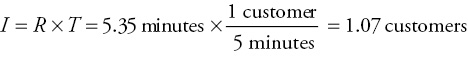
Given that we have calculated the previous individual activity times correctly, we can calculate the average flow time of a customer from getting in line to exiting with their ice cream (i.e., the system flow time) by summing the activity times on the path the customer follows. In the example in Figure 4.2, the system flow time is:
![]()
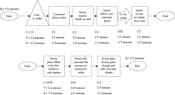
Figure 4.2 Flow diagram of Eis-Sahne Ice Cream Shop
To determine the average inventory of people in line or being served, the manager just adds up the average inventories for each stage in the process. In the example, this is:
![]()
which means that, on average, slightly more than 1 customer is being served at a time. This could also be calculated using Little’s Law for the entire process.
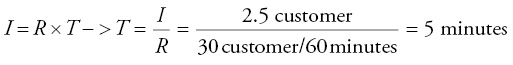
Example: A coffee shop, BeansRUs or BRU, serves 30 custom drinks an hour. The BRU manager has measured the average number of customers waiting for their specialty drink as I = 2.5. Using Little’s Law, this means that the average time a customer waits for a specialty drink is
But what lessons are learned about lean work design by counting the people standing in line at a coffee shop?
Little’s Law shows the relationship of inventory, throughput rate, and flow time to each other. They are not independent of each other.
One of the most important criteria for a customer to choose your service or product, besides quality and cost, is the capability to deliver fast. One possible response to the customers’ preference for fast delivery is to produce in advance and when customer demand arrives, simply give the customer a product from stock. Producing to stock has risks, though. For example, the products produced in advance could become obsolete before they are sold. A “smarter” solution is to reduce the time it takes to produce the product that is, its flow time. This allows a company to be more responsive to customer demand, and as stated by Ohno in the quote at the beginning of the chapter, the company can make more money for example, as it needs to carry less inventory.
Little’s Law clearly shows that the flow time or lead time of a process can be decreased by increasing the throughput rate or reducing the WIP inventory. Typically, companies want to increase their sales and not decrease them; so one of the key objectives of lean work design is to reduce and stabilize the amount of WIP inventory in the process.
One technique that lean companies use to limit the WIP inventory is to create a WIP Cap, which means that once a limit on the number of jobs in process is reached, no additional jobs will be released into the system until the preceding jobs are completed. To explain the rationale behind the use of a WIP Cap, the importance of capacity will be examined.
Capacity
Capacity is an important concept that is related to the throughput rate. In operations management, capacity is defined as the “maximum rate of output for a process, measured in units of output per unit of time” (Hill 2007). In other words, the capacity of a process is the maximum throughput rate (Rmax) that it is possible to achieve.
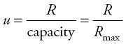
Capacity utilization (u) is the actual throughput rate of a process divided by the capacity of the process.
For example, if we have a grill that can process 1 burger at a time and the processing of each burger takes 5 minutes, then we have a maximum throughput rate of 1 burger/5 minutes or a maximum throughput rate of 12 burgers/hour (i.e., 1 burger/5 minutes times 60 minutes/hour). So the capacity is 12 burgers/hour. If we actually only produce 6 burgers/hour, then we have a capacity utilization of
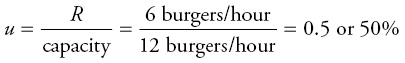
By definition, the actual throughput rate cannot exceed the maximum throughput rate. So, in the preceding example, if the maximum throughput rate is 12 burgers/hour, then we will not be able to prepare 14 burgers during 1 hour. Further, this means that by definition the capacity utilization can never exceed 1.0 that is, 100 percent.
Example: At the BRU coffee shop, 50 customers arrived between 8:00 a.m. and 8:30 a.m. The capacity of BRU is 110 customers an hour. So, between 8:00 a.m. and 8:30 a.m., the arrival rate was 100 customers/hour (i.e., twice 50 customers/hour, since 50 arrived in 30 minutes). This divided by the capacity of 110 customers/hour gives an utilization u of 100/110 = 90.9 percent.
Sometimes, the arrival rate is higher than the long-term capacity of a process. If the manager does not take action, the process will become unstable. In other words, both WIP inventory and flow time will skyrocket. In this situation, managers can either remove some of the demand or obtain more capacity. Obtaining more capacity will reduce the utilization. For example, a manager could assign another worker to the job or the manager could allow overtime, which is one form of capacity increase.
Finally, the capacity minus the throughput rate is the capacity buffer. This is an important concept since it defines the so-called bottleneck of a process.
Most processes use multiple resources to complete the process. All of the resources in the process are unlikely to be utilized to the same extent, in particular, if there is a mix of products produced by the process. Differences in resource utilization within a process occur because each step in a process requires different amounts of time to perform the work and it is very difficult to balance the work across all of the resources. Most processes have a bottleneck resource, which is the one with the smallest capacity buffer—that is, the capacity minus the throughput rate. The bottleneck resource is the resource that limits the throughput of the process.
The neck of a bottle controls how quickly the contents of the bottle can be poured out of the bottle (see Figure 4.3). The body of the bottle has a larger capacity buffer than the bottleneck as illustrated by comparing their respective diameters. The capacity buffer of the bottleneck (i.e., the diameter) limits the rate at which the bottle contents can be poured out. In general, “… a bottleneck is any resource that has capacity less than the demand placed on it.” (Fredendall and Hill 2001; Hill 2007, p. 35).
Little’s Law does not directly consider the capacity of the resource. But, it is helpful to the manager to know the capacity of each resource. This can be done by putting the information into a spreadsheet such as in Table 4.2. In this example, there are four units of resource A. A is the bottleneck, as is seen by comparing its capacity to that of resource B.
In Table 4.2, A is the bottleneck, with a capacity of 0.8 unit/minute or 48 units/hour. If only 0.7 unit/minute of work are arriving, then it has the capacity to do more work than is currently being released to it (i.e., 0.8 unit/minute capacity >0.7 unit/minute being released). Whether this capacity buffer (or excess capacity) might be needed to protect the system from variance (which is discussed in the next chapter), or may be wasted, is up to the manager to investigate. Resource B has more capacity than Resource A since it is a nonbottleneck. Resource B has 1.4 – 0.8 unit/minute of capacity buffer.
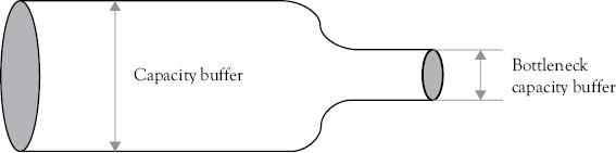
Figure 4.3 Flow rate out of a bottle
Table 4.2 Capacity calculation
| Resource | Resource workload | Unit/time (1/workload) | Number of units of resource | Capacity of resource units/minute | Capacity of resource units/hour |
| A | 5.0 minutes | 1/5 = 0.2 unit/minute | 4 | 0.8 | 48 |
| B | 0.7 minutes | 1/0.7 = 1.4 unit/minute | 1 | 1.4 | 84 |
The capacity of a process is the capacity of its bottleneck resource. This is an important statement. It allows the manager to make another simple observation. If one resource is the bottleneck, then the other resources are nonbottleneck resources. The bottleneck resource will be the resource with the highest capacity utilization. The other resources, that is, the nonbottleneck resources, have lower capacity utilizations than the bottleneck resource (Goldratt and Cox 2004, p. 144). This simple distinction between bottleneck and nonbottleneck resources simplifies the control of the process and focuses the management’s attention on the bottleneck. This view of a process has been popularized by Goldratt in a series of books, but most importantly in a book titled The Goal.
WIP Limit (WIP Cap)
Little’s Law clearly explains the relationship between inventory and flow time. When a manager can estimate the size of the queues a job will encounter during its process, the manager can estimate the total flow time by using Little’s Law. To reduce this flow time, the manager has to reduce the number of jobs waiting in queues or reduce the processing times. The cheapest, fastest flow time improvement comes from reducing the number of jobs waiting in queues (i.e., the work-in-process inventory). The fastest way to do this is to place a limit on the amount of work that can be in the system. Since work cannot be done faster than the bottleneck process rate, it is feasible to limit the amount of work in a system to that required to keep the bottleneck fully utilized. Setting a WIP Cap limits the amount of inventory in a system, which limits the amount of waiting that occurs in the system. Indeed, Hopp and Spearman (2004) consider the WIP Cap to be fundamental to a pull system and define a pull production system as “… one that explicitly limits the amount of WIP that can be in the system” (Hopp and Spearman 2004, p. 142). But this means that the products may have to wait in front of the system. As we learned in the example to Figure 4.1, it is important not to combine the system and the inventory that may be queuing in front of the system. Therefore, it is important to establish appropriate limits for the system for which a WIP Cap is applied.
In the two-stage process illustrated in Figure 4.4, Service Process A is the bottleneck since its capacity is 0.7 customer/minute.
When customers arrive at a faster rate than that and are released into the system immediately upon arrival, the queue in front of Service Process A will become larger. In this example, the queue would grow at the rate of 1.0 arrivals per minute minus 0.7 customer processed, that is, at the rate of 0.3 customer/minute. As can be seen from Figure 4.5, at the end of an hour the queue will increase by 60 minutes multiplied by 0.3 customer/minute or 18 customers!!!
Figure 4.6 depicts the same system as in Figure 4.4 but with a WIP Cap. By placing a WIP Cap on the system, which means not releasing work whenever the total amount of work in the system exceeds a limit, the work in the system remains the same. However, there is a queue or line of unreleased work that is growing at the rate of 0.3 customer/minute (1.0 − 0.7 = 0.3 customer/minute). In other words, the WIP Cap shifts the queue away from the system into a so called pre-shop queue. From the customer’s view point, the wait in the pre-shop queue is not more desirable than waiting within the system, but by controlling where customer orders wait, managers are able to control the process in a considerably easier manner and to predict the flow time of units through the system much more accurately.

Figure 4.4 Two stage process without release

Figure 4.5 Inventory build up
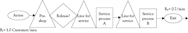
Figure 4.6 Two stage process with release
For the pre-shop queue to be effective, there has to be a period where orders are less than capacity so that the inventory in the pre-shop queue decreases. The pre-shop queue also allows the manager to quickly estimate the waiting time for a job when it arrives at the system. If this is shared with the customer, customers who do not want to wait can go elsewhere. This informs the management about the benefits of purchasing additional capacity, since customers who leave are lost sales.
In the preceding example, by limiting the release of orders in some fashion using a rule such as CONWIP (Hopp and Spearman 2004), which means Constant Work In Process, the number of customers actually undergoing the process remains the same. With a release rule or WIP Cap in place, the manager controls the amount of waiting time in the system. If the manager, in the preceding example, reduces the WIP Cap so there are fewer customers on the shop floor, then while the processing times remain the same, the waiting times decrease. For example if the average inventory in the Service A queue decreases to 0.5, then its waiting time decreases to 0.71 minute. But, note that at the same time the waiting time in the pre-shop pool increases.
Example: A company that does heat treating of partially processed steel parts has found that its customers want an accurate prediction of lead times. To achieve this and to help balance their capacity and workload requirements, they have started to use a WIP Cap by establishing an order release rule that holds jobs in the pre-shop order queue whenever the number of jobs waiting in front of the bottleneck (which is the heat treatment process) exceeds a certain number. They have found that, for two weeks a month, the average arrival rate of jobs is eight a day, but for the last two weeks of a month, the average arrival rate is 12 per day. Their capacity is 10 per day. By putting in a WIP Cap of 10, their pre-shop pool will increase at 2 jobs per day for the 10 working days during the 2-week high demand period or up to 20 jobs. When demand drops during the next 10 working days, the pre-shop pool level will drop to 0, but the shop will keep operating at the same rate. When orders arrive, the shop manager can accurately predict lead times, since the time in the pre-shop pool will be predictable.
Transfer Versus Production Batches
When a process produces in batches, the batch size itself creates waiting time. For example, if the production batch size is 2, then even if the resource is empty when the job arrives, there is waiting time. The first piece in the job starts on time, but the second piece in the job waits until the first job is complete before it starts. In this example, the second job waits 5 minutes, so the average waiting time with a batch size of 2 is 2.5 minutes (i.e., (0 + 5) minute/2). With a batch size of 3, the third job waits 10 minutes, so the average waiting time of each job is 5 minutes (i.e., [0 + 5 + 10] minutes/3). With a batch size of 4 the average waiting time is 7.5 minutes (i.e., [0 + 5 + 10 + 15] minutes/4). This illustrates that as the batch size grows, the waiting time due to the size of the batch also quickly increases. In this example with a batch size of 30, the average waiting time of a job is 72.5 minutes.
While a customer may order a larger batch, it can be processed faster if it is transferred through the shop in smaller transfer batches. That is, because there are fewer jobs in the transfer batch, there will be less waiting due to the batch size.
However, if there are setup times in the process, switching from one large batch to smaller transfer batches can consume capacity as the capacity is used to set up the work stations. In his book, The Goal, Goldratt felt that, in most facilities, this was not a problem because the nonbottlenecks had so much more capacity than the bottleneck. Goldratt recommended that the smaller transfer batches be accumulated at the bottleneck into one large production batch that would again become smaller transfer batches after it was processed on the bottleneck.
Example: Consider the process in Table 4.3. It has four steps, each of which uses a different resource. The jobs arrive in batches of 100, and the processing time at process A, which is the bottleneck is 2 minutes a job. The processing time is 1 minute a job at the remaining three steps. With a batch size of 100, it is 1,000 minutes before the first unit is finished, which is also when the last unit is finished. With a batch size of 10, the first unit is finished in 100 minutes. It is important to note that the setup times are not considered here. The setup times can create significant waiting times when they are large compared to the batch size. Also, while the first units with a batch size of 50 finish at time 500, the last unit may finish at time 1,000 just as when the batch size was 100, unless there are enough resources to process multiple batches at the same time.
Summary
Little’s Law (I = R × T) shows the relationship between the amount of inventory (I), the throughput rate (R), and the flow time (T). This is important to the lean manager, because when the throughput rate is constant, a manager who directs improvement resources on reducing flow time will have to reduce inventory. This will also reduce the costs of the inventory.
Table 4.3 How batch size affects flow time
| Sequence —> | |||||
| A | B | C | D | Time first unit finishes | |
| Processing time per unit | 2 | 1 | 1 | 1 | |
| Batch size 100 | |||||
| Total batch processing time | 200 | 100 | 100 | 100 | |
| Batch waiting time | 200 | 100 | 100 | 100 | |
| Total time to complete process | 400 | 200 | 200 | 200 | 1,000 |
| Batch size 50 | |||||
| Total batch processing time | 100 | 50 | 50 | 50 | |
| Batch waiting time | 100 | 50 | 50 | 50 | |
| Total time to complete process | 200 | 100 | 100 | 100 | 500 |
| Batch size 10 | |||||
| Total batch processing time | 20 | 10 | 10 | 10 | |
| Batch waiting time | 20 | 10 | 10 | 10 | |
| Total time to complete process | 40 | 20 | 20 | 20 | 100 |
It is critical for the manager to recognize where the bottleneck in the process is, since it is the bottleneck resource that dictates the throughput rate of the process. The capacity of the process is the capacity of the bottleneck. So, by recognizing the bottleneck and working to maximize throughput at the bottleneck, the manager is able to maximize the throughput rate of the process.
In situations where demand can exceed capacity, it is useful to establish a WIP Cap, or an order release process, so that not too many jobs get onto the shop floor. Jobs that are not released wait in a pre-shop pool until they are released. This keeps the level of work on the shop floor leveled and makes it possible for the manager to accurately predict the completion times of jobs.
Finally, splitting orders that have multiple units in them into smaller batches of units accelerates the time to the completion of the first units in a batch because it reduces the waiting time at each activity in the job sequence. However, if setup times at the resources are high, the waiting times of each batch may also increased.
References
Fredendall, L.D., and E. Hill. 2001. Basics of Supply Chain Management, APICS Series on Resource Management, Boca Raton, LA: St. Lucie Press.
Goldratt, E.M., and J. Cox. 2004. The Goal: A process of Ongoing Improvement. 3rd ed. Great Barrington, MA: North River Press.
Hill, A.V. 2007. The Encyclopedia of Operations Management, Eden Prairie, NM: Clamshell Beach Press.
Hopp, W.J., and M.L. Spearman. 2004. “To Pull or Not to Pull: What Is the Question?” Manufacturing & Service Operations Management 6, no. 2, pp. 133–48.
Ohno, T. 2013. Taiichi Ohno’s Workplace Management, Special 100th Birthday Edition. English Translation, 2009 by Jon Miller, New York, NY: McGraw-Hill Company.