CHAPTER 5
The Effects of Variance in the System
Reduction of variability is the key to achieving stability. Variability comes in two forms:
Self-inflicted variability—that which you control
External variability, which is primarily related to the customers, but also to suppliers and to the variation that is inherent to the product itself …
Variance is defined by the American Heritage College Dictionary as “a difference between what is expected and what actually occurs.” The previous quote illustrates that there are multiple sources of variance in a process. This implies that there are multiple methods to manage the variation and to eliminate the variation in the system. What an operations manager has to understand, when designing a process, is that variance in the system always reduces the performance of the system.
As you learned from the preceding Chapter 3, a process is a series of operations bringing about a result. These operations are often interrelated, and so there are dependent events in the process. This means that one operation (or a series of operations) must take place before the succeeding operation can occur. So variation in these earlier processes can consequently create variation in the succeeding events. For example, standing in the line at Starbucks, you have to wait until all customers in front of you are served. Thus, your waiting time is dependent on a series of operations (serving the customers in front of you), which have to take place before it is your turn to be served. If one customer in the line takes longer to serve than the average, you will have to wait longer to be served.
To see this, you could count the number in line when you went to order a coffee. If you made a histogram of the number in line over a period of days (see Figure 5.1), you would see that although the average number of customers in line may be 4, that only happened 8 out of the 45 times you measured the length of the waiting line. That means that individual customers have very different waiting line experiences. While the average customer experiences a waiting line of four people, the individual customer experience may be that there was no line or that the line was extremely long.
Looking at only the average value for a process using Little’s Law neglects the amount of variance that exists in the process. While we often know the average value it will take to complete an operation, this completion time is subject to statistical fluctuation or variation. For example, in the Kaffee Shop line, the average time to serve an individual customer may be 1 minute. However, this could be the average of one customer who took 5.5 minutes to serve, and 9 customers who were served in only 0.5 minute each. Or, it could be the average of one customer who took 1.5 minutes to serve, 1 customer who took 0.5 minute to serve and 8 customers who were served in 1 minute each. Both have an average service time of 1 minute but the standard deviation in the first example is 1.4 minutes and in the second example it is 0.24 minutes. While on average each of the 10 customers was served in 1 minute, the variance in the service times and the position of a customer in the line determined their waiting experience. If you were the first in line but in front of the customer who took 5.5 minutes to order, your waiting times would be short. However, if you were the customer who was waiting behind the customer who took 5.5 minutes to order, you would experience a longer waiting time.
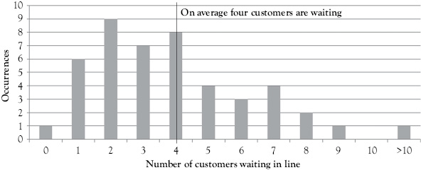
Figure 5.1 Histogram of customers waiting to order
A major problem with variance is that it propagates if operations depend on each other. This is illustrated in the following example.
Example: Tom, Bob, and Mary are to analyze the ice-cream market to determine customer preferences and present a report in six days. They decide to divide the work between themselves. Tom is to gather the data from the market, Bob will take the data from Tom and analyze it, and Mary will take Bob’s analysis and prepare the presentation. Tom, Bob, and Mary scheduled two days for each of their steps. However, it turns out that the data is harder to get than expected. Tom needs three days instead of two days. Bob tried to do his analysis faster to make up for Tom’s delay, but Bob took an entire two days to do the analysis. So, Mary did not receive Bob’s analysis until a day later than planned. So, Mary has only one day in which to complete two days of work.
If the deadline that Mary faces is a “hard” deadline for the presentation, then she has to work over time. This is illustrated in the Gantt chart in Table 5.1 showing the actual versus the expected performance. The sequence dependence in the process means that Mary could not start work early and that the delay that started with Tom is passed from Tom to Mary.
Assignable Versus Common Variability
Following Liker and Meier (2006) variability comes in two forms: (1) self-inflicted variability, which can be controlled; and (2) external variability. This categorization of variability is similar to the difference between common and assignable variability introduced by Shewhart (1931) and Deming (1986). Shewhart (1931) argued that each controlled capability is variable. A capability is said to be under control when, through the use of past experience, one can predict, at least within limits, how its target condition may be expected to vary in the future. Prediction within limits means that the probability that the observed measure for the target condition will be within the given limits can be stated at least approximately. It follows that a controlled process is a constant system of chance causes. However, it was found that there are causes of variability that do not belong to a constant system. It was further found that these causes can be assigned to special causes, and assignable (or special) causes of variation can be found and eliminated.
Table 5.1 Analysis ice-cream market—estimated versus actual
| Days in process | |||||||||
| Resource | Activity | 1 | 2 | 3 | 4 | 5 | 6 | 7 | |
| Tom | Gather market data | Estimated | |||||||
| Actual | |||||||||
| Bob | Analyze market data | Estimated | |||||||
| Actual | |||||||||
| Mary | Prepare presentation | Estimated | |||||||
| Actual | |||||||||
The measures to reduce variability are determined by the type of variability. Based on the aforementioned, variability can be classified into three categories as follows:
Assignable variability can be found and eliminated through improvement bringing the process under control. If a process is under control, a company will reach its operating frontier.
Common variability of the infrastructure can only be reduced by infrastructural change.
Common variability of the physical asset can only be reduced by radical technological upgrades or replacements.
Interaction of Variance and Utilization
In the previous examples, a fundamental concept that was not explicitly explained was utilization. The process always has trouble if variance in demand affects the bottleneck. If demand on the bottleneck resource is less than expected, then the bottleneck is starved for work. If demand is greater than expected, the bottleneck resource has more work than it can do. So, the bottleneck is an important control point for the manager of a process.
Kingman (1961) quantified this relationship between variance and utilization for one work station in the following equation.
|
(5.1) |
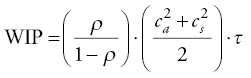
where
ρ = utilization
ca2 = coefficient of variation of arrivals (demand variance)
cs2 = coefficient of variation of service time (process variance)
τ = is the average flow time
WIP is the amount of inventory in line in front of the work station. The coefficient of variation is the standard deviation divided by the average. It is used because it normalizes the standard deviation. Dividing the sum of the two squared coefficients of variation together, we get the average squared coefficient of variation.
Note that all customers or jobs have to be served by the same capacity resource—thus operations are dependent. Further, Equation 5.1 consists of three terms: utilization, statistical fluctuation or variance, and the mean flow time. This means that the flow time (i.e., service time) increases as a multiple of the utilization level and the variance level. As aforediscussed, when the variance is high, the utilization level must be much lower to provide the same level of service. As the level of variance is decreased, the size of the capacity buffer can be reduced because there is less likelihood of delays due to variance in the system. So a key principle of lean work design is to establish a process that minimizes deviation from a target value, and a design that also allows deviation from target value to be quickly identified and corrected.
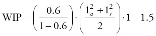
For example, if the processing time at the resource is 1.0 time units and the resource utilization is 50 percent with a coefficient of variation of arrivals, ca2, of 1 and coefficient of variation of processing times, cs2, of 1, then:
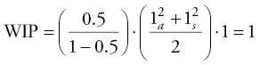
This means that even with only 50 percent utilization of this resource, the variance in the system (both the variance in arrivals and the variance in processing times) will cause an average of 1 unit or 1 person to be in line waiting to be processed. If the arrivals are from outside of the system then this variation may not be in our control. For example if the arrival variation is a measure of customer arrivals we may not have control. However, the variance in processing times may be within our control and, as described in the quotation at the beginning of the chapter, may be a self-inflicted variance.
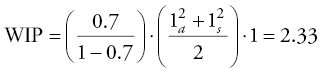
If the variance in the preceding example remains the same, but the utilization increases from 50 percent to 60 percent, the WIP is then:
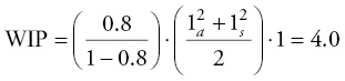
So there was a 50 percent increase in the number in line, while there was only a 10 percent increase in the utilization level. If the utilization increases further to 70 percent, the WIP is:
Again if the utilization increases another 10 percent to 80 percent, the WIP is:
As the utilization increases another 10 percent to 90 percent, the WIP is:
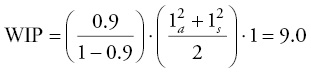
Table 5.2 Effect on WIP of interaction of server utilization and variation with processing time, T = 1
| Utilization level | Coefficient of variation in arrivals = 1.0 Processing time = 1.0 | Coefficient of variation in arrivals = 0.5 Processing time = 1.0 | Coefficient of variation in arrivals = 0.5 Processing time = 0.5 | Coefficient of variation in arrivals = 0.25 Processing time=0.25 |
| 0.5 | 1.0 | 0.6 | 0.3 | 0.1 |
| 0.6 | 1.5 | 0.9 | 0.4 | 0.1 |
| 0.7 | 2.3 | 1.5 | 0.6 | 0.1 |
| 0.8 | 4.0 | 2.5 | 1.0 | 0.3 |
| 0.9 | 9.0 | 5.6 | 2.3 | 0.6 |
| 0.95 | 19.0 | 11.9 | 4.8 | 1.2 |
So, there is an exponential increase in the WIP as the utilization increases. But this effect is even worse than it looks at the first sight since the WIP calculated is the average. Since even for a 90 percent utilization the waiting time is zero in 10 percent of the cases, the increase in waiting times occurs in the form of extreme waiting times. In other words, the histogram in Figure 5.1 shows a much longer tail on the right hand side.
Table 5.2 shows the corresponding decreases in the amount of WIP as the coefficient of variation decreases for any given utilization level. For example, at the 0.5 or 50 percent utilization level, the WIP decreases from 1.0 to 0.6 as the arrival coefficient of variation is decreased and to 0.3 when the processing time coefficient of variation is also decreased to 0.5. When both coefficients of variations are decreased to 0.25, the WIP for 50 percent utilization is decreased to 0.1. As the utilization increases, the WIP increases for each setting of the coefficients of variation in arrivals and processing time.
This relationship is illustrated in Figure 5.2. Figure 5.2 is a graph of the data in Table 5.2. This shows that the increase of WIP is much larger as the utilization increases when the combined coefficient of variation is larger. For example, in Figure 5.2, when the coefficient of variation of arrivals is 1.0 and the coefficient of variation of processing times is 1.0, the WIP is much higher at a 95 percent level than the WIP for 95 percent utilization with both the coefficients of variation of arrivals and processing time at 0.25. This indicates that a resource with low coefficient of variation in arrivals and processing times can perform better than those systems with higher variance especially at higher levels of utilization. Notice that at 95 percent utilization WIP is only 1.2 with the coefficients of variation of arrivals and processing times at 0.25, but with the coefficients of variation of arrivals and processing times at 1.0, the WIP is 1.5 at the 60 percent utilization level. This underlines the importance of considering and, if possible, reducing or avoiding variance in a lean work design.
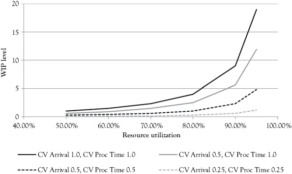
Figure 5.2 Effect on WIP of interaction of server utilization variation with processing time, T = 1
Protecting Throughput from Variance
Often, ensuring system throughput means ensuring the bottleneck throughput. The key point for a process manager to remember is that the capacity of the bottleneck resource restricts the entire system’s performance. As the bottleneck capacity utilization comes closer to 100 percent, there is less capacity left to overcome statistical fluctuations of preceding resources. Without a capacity buffer, any delays prior to the bottleneck resource create delays at the bottleneck, and if the bottleneck does not have the capacity to overcome the delays, then the process throughput is reduced. The nonbottleneck resources can have protective capacity, which is the amount of capacity they have in addition to the capacity of the bottleneck. The bottleneck can have safety capacity, which is the amount of capacity the bottleneck has that is in excess of demand. This is illustrated in Figure 5.3. As the safety capacity decreases (which means that utilization is increasing), then the only capacity buffer in the system is the protective capacity at the nonbottlenecks.
When designing the system, the manager must make a decision about how much safety capacity and how much protective capacity to have. One heuristic is that the safety capacity at the bottleneck is to protect the throughput from variance in the customer demand. The protective capacity is used to protect the system from variance inside the process. One simple approach is to use the nonbottleneck protective capacity in front of the bottleneck to create an inventory in front of the bottleneck. This allows the bottleneck to continue working without starvation from the lack of work if there is a delay in another part of the system. Protective capacity after the bottleneck is typically less effective. In fact, it cannot be used to ensure throughput at the bottleneck, but can be used only to speed up a process, which is delayed at the bottleneck, for example, to meet due dates.
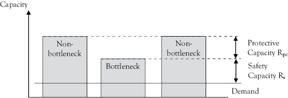
Figure 5.3 Protective capacity versus safety capacity
Another technique to improve process throughput is to have flexible resources. In this way, more capacity can be added to the bottleneck when it is needed. For example, at some coffee shops when the line gets long, a second server may come and start taking orders from people several steps away from the first server. They might say something such as: “Good morning, can I start preparing your drink in advance?” Once they have the order they will start preparing the order, so it is already at the cash register when the customer reaches the front of the line. Or another technique to solve the problem of sequence dependence is to put all of those who have simple orders, such as only coffee, into a separate queue. This is often seen at grocery stores where one register may be reserved for small orders of “10 Items or Less.”
In the coffee shop example, the managers are solving the problem by bringing extra capacity from a process that is currently not the bottleneck to assist the bottleneck process. So, the workers who start taking preorders and getting orders ready are doing tasks that the bottleneck was doing so that now the bottleneck has to do less work per customer. This is illustrated in Figure 5.4. The flexibility of the nonbottleneck resource increases the capacity of the bottleneck as shown by comparing the “Before” to the “After” picture.
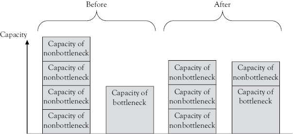
Figure 5.4 Adjusting bottleneck capacity
References
Deming, E.W. 1986. Out of the Crisis. 2nd ed. Cambridge, MA: Massachusetts Institute of Technology.
Kingman, J.F.C. 1961. “The Single Server Queue in Heavy Traffic.” Proceedings of the Cambridge Philosophical Society 57, no. 4, pp. 902–4.
Liker, J.K., and D. Meier. 2006. The Toyota Way Fieldbook: A Practical Guide for Implementing Toyota’s 4Ps. New York, NY: McGraw-Hill.
Shewhart, W.A. 1931. Economic Control of Quality of Manufactured Product. 50th Anniversary Commemorative Reissue, American Society for Quality Control, Chelsea, MI.