CHAPTER 6
Buffer Management
For parts that are going through bottlenecks, queue is the dominant portion [of their time in the plant]. The part is stuck in front of the bottleneck for a long time. For parts that are only going through non-bottlenecks, wait is dominant, because they are waiting in front of assembly for parts that are coming from the bottlenecks. Which means that in each case, the bottlenecks are what dictate this elapsed time. Which, in turn, means the bottlenecks dictate inventory as well as throughput.
Given that every system has variance and that variance negatively affects the performance of the system, all work designs need to address how to limit, control, or buffer the variance to protect throughput. As illustrated in the previous quote, the majority of the time work spends inside a system is usually not processing time. It is time queuing for work to be done, or it is time spent waiting for another part to be prepared. While the previous chapter focused on variance and provided examples of variance reduction, this chapter focuses on how to buffer variance to effectively protect system throughput.
The buffers that protect a system from variance are directly related to each other and to throughput using Little’s Law. There are three types of buffers in any system—inventory, lead time, and capacity (Hopp and Spearman 2004). The inventory buffer is any inventory that is used to protect the system throughput from variance in either the demand or the process. The safety capacity buffer is extra capacity (i.e., capacity greater than average demand) that is used to protect throughput from variations in demand or in the process. The lead time buffer is additional time in excess of the expected time to produce the product or service.
The first important take away from the recognition that variance must be buffered is—if we can minimize variance, we have less need to use buffers. So, an important consideration of lean work design is how the process design itself can minimize variance in the process. A second take away is that variance is due not only to the internal process but also to external demand. Customers may not want to order in a stable pattern. But, reducing the variance in either the demand or the process reduces costs by allowing for smaller buffers. While variance reduction is one of the most important principles in lean work design, not all variance can be avoided since it may be what the customer buys (e.g., customized orders made-to-order).
One of the most important buffers in any system is the capacity buffer. As Figure 5.3 in Chapter 5 illustrated, there are two types of capacity buffers and they have to be managed differently. The safety capacity buffer (Rs) is the additional capacity at the bottleneck that exceeds the average demand (on the bottleneck). An important first point is that safety capacity is only at the bottleneck process. A second important point is that to have safety capacity, the bottleneck cannot be scheduled at 100 percent of its capacity. Meanwhile the nonbottlenecks have more capacity than the bottleneck. That portion of their capacity that exceeds the bottleneck’s capacity is their protective capacity. This means that the protective capacity (Rpc) is different from safety capacity and is that capacity at the nonbottlenecks that exceeds the bottleneck capacity. This protective capacity allows the nonbottlenecks to protect production at the bottleneck. It is by managing the utilization of these capacities that the manager determines how much time work spends in queue.
The time in queue is controlled by the manager limiting the production of the nonbottleneck resources to what is essential to keeping the bottleneck working at its scheduled rate. The bottleneck is scheduled to work at the rate that the customer is demanding a service or product, so the nonbottleneck has to be viewed as a support resource. The non bottleneck can produce inventory in advance of the bottleneck as an inventory buffer to keep the bottleneck working in case there is a disruption in the production process leading up to the bottleneck, but this inventory buffer in front of the bottleneck has to be controlled so that the queuing does not become excessive. This is illustrated in Figure 6.1.
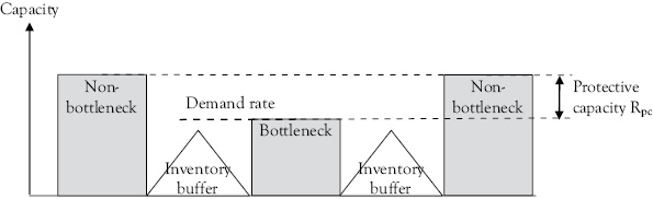
Figure 6.1 Unbalanced flow line with protective capacity and inventory buffers before and after the bottleneck
An important point observed from Figure 6.1 is that by using the protective capacity of the nonbottlenecks to protect the bottleneck from system variance, the inventory buffer can be kept relatively small. The bottleneck is still protected from the negative effects of system variance, but there is not an excessively long queueing time.
The queue that follows the bottleneck is an inventory buffer (Ibuffer) that also protects the bottleneck by ensuring that there is someplace to put the output that the bottleneck processed. This prevents the bottleneck from being blocked if there are delays downstream (i.e., at the succeeding stations) from it. To ensure the queue does not grow excessively, it has to be monitored and managed.
Example: A hospital X-ray facility asks the Medical-Surgical floor nurses to bring patients who need X-rays to their lab 10 minutes before their scheduled times for their tests. This keeps a small buffer of patients who are waiting and ensures that production of the X-ray tests is not starved because no patients are waiting. However, if the X-ray process itself slows down for any of multiple reasons and no one informs the Medical-Surgical floor nurses that the procedures are delayed, then the queue of patients waiting for tests will start to grow very long. This congestion creates long queuing times that soon exceed the time required to undergo the X-ray tests, just as in the quote at the start of the chapter.
Actual processes always have variance. Managers need to use the system tools to manage the system response to this variance. By default if management does not control the system, there will be longer flow times, higher utilization and higher inventory. The point is that if managers do not control where the buffers are placed within the system, the buffers will emerge as an outcome of the interaction of the demand and the resource performance. A lean work design includes decisions about:
How the system is to be protected from variance; and
How to prevent variance.
First, a simple example about variance and buffers to protect the system from variance will be used to explain how to incorporate buffers into the work design.
Example: You have to complete a homework assignment whose deadline is in two days. In this class you have found during the semester that it takes an average of 1 hour to complete a homework assignment. You know that you have 5 hours of study capacity each day and that tomorrow you need only 2 hours to study for a test the day after tomorrow in a different class and another 2 hours to read a case and prepare an analysis for a third class. You decide to wait until tomorrow to complete the homework assignment. This means that you have decided to reduce the lead time buffer from one day to zero days (i.e., currently your lead time is two days for the homework assignment, but you will not start it until tomorrow, and it will take one day to do). This decision to put off the homework assignment until tomorrow does not increase your finished goods inventory buffer, since nothing will be completed. You also decided to have no capacity buffer, since you have completely scheduled all of your capacity. On the next day, when you start the homework assignment, you discover that it will take more time than the 1 hour you scheduled for it. Since you want to study for the test and complete the case analysis, you decide to work all night to get the work done (i.e., you obtain more capacity). While this decision increases your capacity in the short term, it also reduces your capacity in the next days because of the sleep deprivation, which will have to be made up.
As in the preceding example, depending on our decisions the buffers are interchangeable. We could have started the homework assignment a day earlier and used the lead time buffer. If we had completed the assignment the day before, we would have created an inventory buffer, since the homework would be there in the buffer for us to be handed over to the professor on the due date. Also, when we registered for classes, we could have created a larger capacity buffer by taking fewer classes.
Managers can use the insights that all systems have variability buffers that consist of some combination of inventory, capacity, and time to improve the operations of all of their processes. The key is to understand that part of their work design requirements is to eliminate variability if possible or, if not possible, to have the correct mix of variability buffers in place. In the previous example, while the homework assignments take an average of 1 hour each, some are longer and some are shorter. Since the average time to complete an assignment was 1 hour, there was a 50 percent possibility that any individual assignment will take longer than the average to complete it. Managers determine the target level of each buffer in line with the target capabilities of the process. For example, if the target is to produce a certain product within a certain time, this target determines how capacity has to be assigned, the level of inventory, and the size of the lead time buffer. In the preceding example, if I wanted to get a good night’s sleep each night and do well in all my classes, I could decide to never fully schedule all of my study capacity, so that I always had at least a 1-hour safety capacity buffer. I could also decide to complete all home works at least one day in advance to create a one-day lead time buffer. If I did this, I would then create a finished goods inventory buffer of completed home works.
The previous examples are to illustrate that managers can establish targets for the system buffers and measure how close the buffers are to their target level. The targets become standards against which the system can be measured. The ability of the system to operate at these target levels determines the capability of the system, where capability is the ability to perform specific tasks. This is illustrated in Figure 6.2.
The critical task of the manager is to ensure that through these decisions the organization remains competitive. So, buffer management consists of three interdependent steps (see Figure 6.2). Managers need to determine the level and type of buffer required. This is a clear statement by the manager of how they intend to compete. Is it important that they have customer service times that are equal to or less than their competition? Or is it more important that they have the lowest costs? Capacity costs money. So often the trade-off is between longer customer waiting times and lower costs.
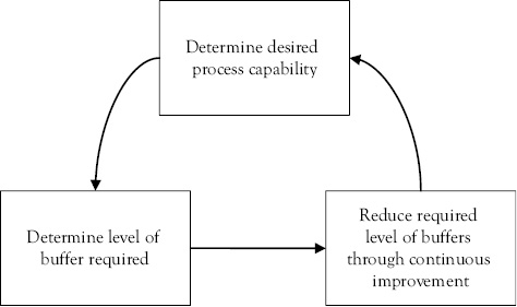
Figure 6.2 Buffer management
Example: A supermarket manager determined that the customers the store wants to attract are willing to pay a small premium for convenience. So, the manager may set a target queue size of three customers waiting in line at a cash register. This would be a smaller queue than the nearest competitors. The manager then gives instructions to the cashiers that anytime their queue exceeds three customers they should request assistance. At that point the assistant store manager will come and immediately open another line for the customers.
By doing this, the manager is using the assistant store manager as safety capacity for the cashier process. The store managers can track the number of times the assistant manager has been called to help the cashiers, and how long the assistant managers works at the cash register once they arrive. This gives the store manager information about the utilization of the buffers and the correct cashier capacity to maintain the desired queue size of customers. The targets that the manager selects for the buffer sizes are those that keep it competitive or allow it to have a competitive advantage.
By tracking and adjusting the buffer sizes, the manager is continually adjusting to the competitors’ actions and the system outputs.
This has been expressed in a different way by Goldratt and Cox (2004) in their book The Goal, in what Goldratt and Cox call the Theory of Constraints. Goldratt views the primary objective of the manger as ensuring throughput, where throughput is the rate at which a system accomplishes work, that is, generates money through sales, or the rate at which money comes in. The focus on the rate at which sales are obtained has the important characteristic of focusing the managers’ attention on how to support sales by adding value in the most effective way possible.
To ensure throughput targets are met or exceeded, management has to set the level of buffers at the appropriate level. Once throughput is ensured the manager can then find ways to minimize inventory and operational expenses as long as the changes do not negatively affect throughput. So, managers must not only increase throughput, they should, preferably, do it while reducing inventory and decreasing operating expenses. In Goldratt’s terms, inventory is all the money that the system has invested in purchasing things, which it intends to sell (this is the money that is captured within the system). Operational expense is all the money the system spends in order to turn inventory into throughput.
Example: The manager of Eis-Sahne has decided that on a hot Friday night, there will be demand for 20 ice-cream cones an hour and that on average each of these will take 5 minutes to prepare and give to the customer. The manager has decided to have a clerk who is separate from the creamistas (i.e., the persons who prepare ice-cream cones for customers) and who will take the order and receive the money. It only takes the clerk 2 minutes on average to take the order and the money. This means that the protective capacity of this clerk is 20 minutes an hour (i.e., 60 − 2 * 20 = 20 minutes). Also, the manager has created the creamistas a safety capacity of 2 * 60 − 5 * 20 = 20 minutes. The safety capacity is the difference between the average demand placed on the creamistas and their capacity, since they constitute the bottleneck. If the manager places a sign at the beginning of the line that says once you enter your order you will get your ice cream cone in 10 minutes whether you wait quietly or shout loudly, the manager has provided an average lead time buffer of 5 minutes (i.e., 10 − 5 minutes creamistas processing time = 5 minutes).
In this system, the average throughput will be the average sales less the average cost of the ice cream and cones. If the average sales price is $5.00 and the average cost of the ice cream and cone is $2.00, the average throughput of a sale is $3.00. This means that the average throughput an hour is $3.00 * 20 cones/hour = $60.00 an hour.
The objective of work design is to balance the throughput—or the flow of work through the system—with the demand from the market. The definition of bottleneck makes it clear that the bottleneck flow should be aligned with this demand (Goldratt and Cox 2004, p. 145). Thus if bottlenecks exist, one can even use them to control the flow through the system and align this flow with the market. Once a constraint is identified, lean work design seeks to reduce variance to the constraint and to buffer the constraint. The manager can also use lean work design to overcome the constraint by redesigning the process to reduce the buffers and reduce the costs (i.e., inventory and operational expenses).
It is the manager’s job to continuously improve the work design. That means that the manager has to continuously tweak the work design so that it serves the customer better, and so that the buffers and their costs are continuously reduced. The ensuing quotation serves to illustrate this point.
At the gathering, various people talked about the good old days. About half-way through the meal, I overheard Mr. Ohno say to his neighbor, Mr Takimura ….
“All right, Takimura! Go ahead and keep a little stock around. After all, the crucial thing is for the company to make money.”
Knowing that Mr Ohno viewed stock as his archenemy, I was shocked to hear him tell someone that it was all right to keep inventory at hand. My surprise, however, merely added to the impact of his true intentions as revealed in his next sentence:
“However, don’t think that it is all right to keep stock around forever!”
All too often, we tolerate stock as long as we are making money and, in no time at all, come to accept inventory as a fact of life. What impressed me in Mr. Ohno’s words, by contrast, was his aggressive attitude toward making fundamental improvements:
“Current conditions may make it necessary to keep stocks around right now; but keeping them is inherently wasteful, and you will have to find ways to make money without carrying inventory at some point.” (Shingo 1989, p. 140)
Example: The new manager of the hospital X-ray unit decides that the patient and their insurance company is their customer and, in an effort to increase patient satisfaction with their services, starts to measure the number of patients waiting for their services. They discover that the average number of patients waiting for their services is six. Given that their average throughput is 5 patients an hour, this means that the average patient waits in the queue for 1.2 hours (T = I/R = 6 patients/5 patients/hour), which seems excessive since these are sick patients waiting together in a queue. The manager discovers that while the average X-ray processing time is 12 minutes, there is a standard deviation of 3 minutes for each X-ray service. This means that the X-ray machine, which is the bottleneck, is scheduled so that there is no safety capacity. Upon further investigation the manager discovered that the X-ray technicians often worked through their breaks and through their lunch period to keep the number of patients in line to a minimum. This meant that the X-ray technicians were adding capacity to the process.
The first intervention the new manager did was to have the registration clerk notify the nursing floors not to send more patients when the number of patients in line was three or more. This action reduced the patient queuing time and reduced physical congestion in the unit.
The second intervention the new manager did was to examine what was causing the 3 minute standard deviation in the X-ray service. As they studied the process, the technicians and manager discovered they could reduce the average time to 11 minutes and reduce the standard deviation to 2 minutes. This provided some safety capacity (60 − 5 patients/hour * 11 minutes/patient = 5 minutes safety capacity an hour). This was still not adequate safety capacity given the service standard deviation of 2 minutes, since the standard deviation an hour was 4.5 (s = 2√5) leaving almost no safety capacity (i.e., only 0.5 minutes).
The third intervention the new manager did was to promise not to schedule the X-ray service at 100 percent utilization, so that if further improvement could be found to decrease the processing time, the staff would benefit from having an improved buffer. The staff and the manager continued to work on their process and were able to reduce the service time to 10.5 minutes and reduce the standard deviation to 1.5 minutes. This resulted in a safety capacity of 7.5 minutes (60 − 5 * 10.5), which was slightly larger than the standard deviation of 3.35 minutes an hour).
The point of the preceding example is that the manager needs to intervene repeatedly to accomplish the goal of having a system that responds to the customers’ needs while keeping operating expenses within control. The manager needs to be able to measure the effects of the interventions on both the variance and the buffers. Finally, the manager controls the size of the buffers through decisions about arrival rates and interventions in the process of doing the work.
References
Goldratt, E.M., and J. Cox. 2004. The Goal: A Process of Ongoing Improvement. 3rd revised ed. Great Barrington, MA: North River Press.
Hopp, W.J., and M.L. Spearman. 2004. “To Pull or Not to Pull: What Is the Question?” Manufacturing & Service Operations Management 6, no. 2, pp. 133–48.
Shingo, S. 1989. A Study of the Toyota Production System from and Industrial Engineering Viewpoint. 1st revised ed. Cambridge, MA: Productivity Press.