
12
Dynamic Programming for Stereo Matching
So far, we have discussed the following concepts: vision simulator (Chapter 4), stereo matching (Chapter 6), and DP machine (Chapter 9). As one of our final goals, in this chapter, we explain how to design a DP machine for stereo matching (Baker and Binford 1981; Ohta and Kanade 1985).
There are various types of stereo DP machines. One possible source of diversity is the reference system: left, right, or center. The various types of DP machines may have some parts of their code in common, but they may also have some dissimilar code that is reference-system-dependent. A good design contains as much code as possible in common, keeping the number of reference-system-dependent parts as small as possible. Another possible source of diversity is the number of processors: single processor or array processor. In a single processor system, all the computation is carried out within the same processor. The processor is actually a large FSM, driven only by a clock and a reset signal, together with RAMs storing the left and right images and the disparity map. On the other hand, in an array processor system, all computation is carried out via a network of identical processors. In this case, there must be a plan for supplying the images to the network, retrieving the disparity maps, and executing each processor in various states. Yet another possible source of diversity is the use of lines: one line or a set of lines. A minimal system may use only a pair of image lines for stereo matching. A more advanced system may use a set of image lines from both left and right images to compute neighborhood operations.
In this chapter, we explain how to design a DP machine for stereo matching, for the left and right reference systems, a single processor, and neighborhood computation. The reference systems can be selected by the Verilog compiler directives, making the three systems into the same Verilog HDL code. We review the stereo matching algorithm, hypothesize a DP machine, and design Verilog codes.
12.1 Search Space
We start again with the space in which the solution exists. The space consists of the points, {(x, d)|x ∈ [0, N − 1], d ∈ [0, D − 1]} for the left right reference and {(x, d)|x ∈ [0, 2N − 1], d ∈ [0, D − 1]} for the center reference system (Figure 12.1). The first property of the disparity is that it depends on the reference system and thus must be explained in a general setting.
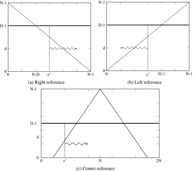
Figure 12.1 The (x, d) space: left/right and center reference systems
The second property is that the solution space must be further confined to the trapezoidal region within the rectangular space. This is because only points in this region can be observed by both images. Outside of this region, all the points are indeterminate, due to lack of observation. Consequently, when we consider the space as a graph, we call the observable nodes matching nodes and the unobservable nodes occlusion nodes. In the center reference system, occlusion nodes exist even inside the trapezoidal region. Both types of nodes are alternately distributed in this region. The identity of a node can be easily verified by observing whether x + d is even or odd. (It depends on where the node origin is defined. For an x ∈ [0, 2N] system, it is odd and for an x ∈ [0, 2N − 2] system, it is even.) If the domain is defined as x ∈ [0, 2N], x + d is odd. The corresponding coordinates in the images are xr = (x − d − 1)/2 and xl = (x + d − 1)/2. If the domain is x ∈ [0, 2N − 2], x + d is odd. The corresponding image points are xr = (x − d)/2 and xl = (x + d)/2 (refer to Equation (6.80)). In designing the circuit, we need to know where the matching nodes are. If we represent such regions by Rr, Rl, and Rc, they are given by
In order to find a feasible solution in the solution space, we can embed all the paths that we are looking for. In this manner, the search space can be defined over the solution space. To make the method clearer, we can represent the search method by a graph, G = (V, E), which consists of nodes and edges (Figure 12.2). The nodes are the lattice points in Figure 12.1 and the edges are the feasible path of the desired object boundary. This graph is specific in that the edges are connected between adjacent nodes only, although there could be many other connections. This particular graph is very limited but also efficient in DP realization.
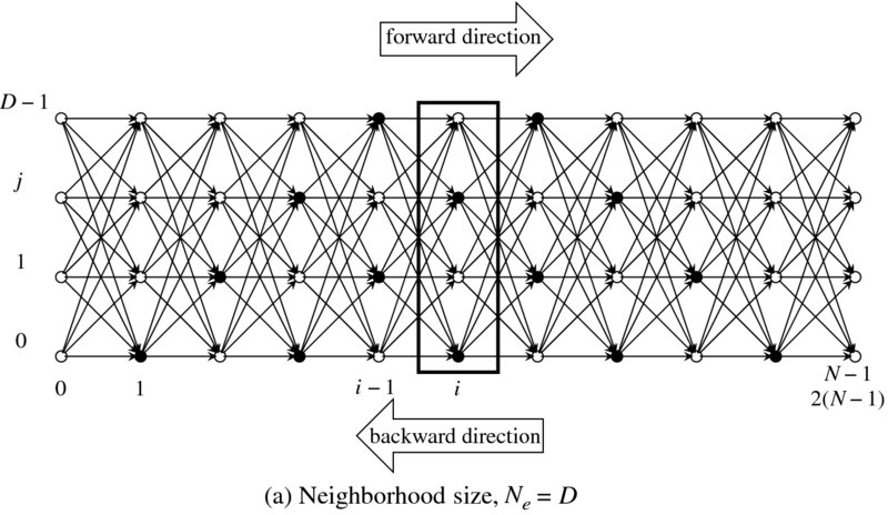
Figure 12.2 A graph for the search spaces. The size is either D × N or 2D × (N − 1)
The graph consists of DN nodes for left right references and 2D(N − 1) nodes for center reference. Some nodes are in the trapezoid; these are called matching nodes, and some others, called occlusion nodes, are not. This graph shows the center reference as an example. The strategy is to compute column by column, as the nodes in a column are represented by a block in the figure.
From the previous two figures, we obtain the local connections, as shown in Figure 12.3. On the left a connection in the right or left reference system is shown. Any pair of nodes connected by the edge are assigned uniquely in different positions in the right or left image planes: (x − 1) and x. The figure on the right side is the possible paths in the center reference system. If the coordinates are mapped to the image plane, the nodes (xc − 1, d − 1) and (xc, d) are mapped to the same position in the right image plane (see Equation (6.80)). They are actually (x, d − 1) and (x, d) in the left right reference, a path that is prohibited in the search path. Similarly, the nodes (xc − 1, d + 1) and (xc, d) are actually the same point in the left image plane. They are the points, (x, d − 1) and (x, d), which must be avoided in building the search path. The search space of the center reference is the one skewed from the left right reference system. That is, (x, d − 1) and (x, d) are mapped to either (xc − 1, d − 1) and (xc, d) or (xc − 1, d + 1) and (xc, d) in the graph. We must expect the result of the center reference system to be very unreliable compared to that of the left right system.
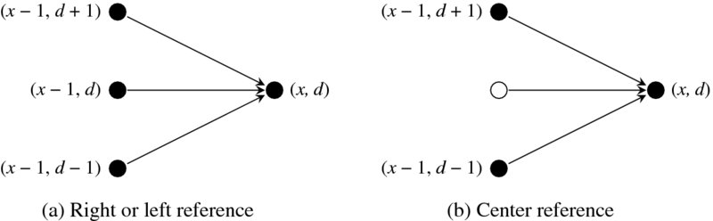
Figure 12.3 Two cases of connections: (a) x + d = odd (b) x + d = even
12.2 Line Processing
From a computational point of view, a pair of conjugate images can be processed in one of three ways: line, strip, or plane (or frame). In the first method, the image is scanned in raster manner and processed for disparity computation between the line intervals. In the second method, the line is expanded to a block of lines, which shifts downwards in an overlapped or skipped manner. Finally, in the third method, the entire image plane is processed as a body. Before going any further, let us first define this concept.
For the image plane, ![]() , the three schemes can be illustrated as depicted in Figure 12.4. Figure 12.4(a) depicts the three images, Il( ·, y), Ir( ·, y), and disparity d( ·, y). The computation uses the images on the epipolar lines, producing disparity on the same line:
, the three schemes can be illustrated as depicted in Figure 12.4. Figure 12.4(a) depicts the three images, Il( ·, y), Ir( ·, y), and disparity d( ·, y). The computation uses the images on the epipolar lines, producing disparity on the same line:
Here, T( · ) represents the disparity computation operations. The computation progresses downwards line by line. In Figure 12.4(b), the line is expanded to a set of lines, {Il( ·, y′)|y′ ∈ [y − (L − 1)/2, y + (L − 1)/2]} and {Ir( ·, y′)|y′ ∈ [y − (L − 1)/2, y + (L − 1)/2]}, and disparity d( ·, y). In this case, the disparity computation becomes
Using more than one line potentially facilitates neighborhood computation. To make the strip symmetric on both sides of the centerline, the number of lines in a strip, L, must be an odd number. If L = 1, the strip becomes a line. If L = M, the image frame itself is signified.
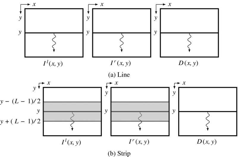
Figure 12.4 Computing line and strip: left image (Il), right image (Ir), and disparity map D
Because the computation progresses downwards, the disparities of the previous lines are available to the current line and thus recursive computation is made possible:
Using the previous disparity may help in deciding the disparity of the present line.
In light of this, in designing the DP machine, we have to consider the computation structure (multiple lines, neighborhood computation, and recursive computation) and leave the details to the actual algorithm design.
12.3 Computational Space
As discussed in Chapter 6, the stereo images can be referenced in terms of the three coordinates system: left, right, and center reference. To design appropriate DP machines, we have to know the search space of these systems in detail.
Figure 12.5 shows the space observed by two cameras. The space containing the observed sites (black dots) is the epiplane, and the horizontal axis is the epipolar line. The apex of the inverted triangle is the nearest point with disparity N − 1, while the base of the triangle and beyond are the farthest points with disparity zero. This space can be viewed from many directions, such as the right image axis, the left image axis, and the center between the two images, as illustrated. As a result, we can derive spaces (xr, d), (xl, d), and (xc, d), respectively called right reference, left reference, and center reference system.
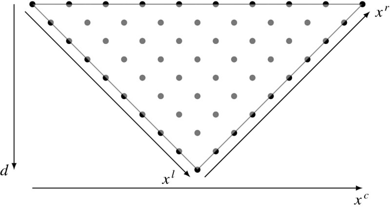
Figure 12.5 An epiplane plane and three coordinates: right, left, and center reference images (the disparity is shown as an inverse of the depth)
In the right reference system, the image on the right is used as the reference in computing the distance:
where d denotes disparity and xl denote the coordinates in the left image. Similarly, in the left reference system, the image on the left is used as the reference in computing the disparity:
where xr are the coordinates in the right image plane. Note the difference in the sign placed before the disparity. Notice the difference in the sign attached before the disparity. In the center reference system (Jeong and Oh 2000; Jeong and Park 2004; Jeong and Yuns 2000; Jeong et al. 2002), the corresponding points are
where xc are the coordinates in the center reference system. After the disparity is obtained, it can be mapped to the coordinates in the left or right image planes, according to Equation (6.80),
We will sometimes call the mapped coordinates, respectively, center left reference and center right reference, for convenience. The places where the occlusion nodes exist are the other positions that do not satisfy this condition. Those positions can be used for smoothing purposes, as we shall see.
Collectively, we can define a space (x, d), consisting of the coordinates and disparity, and examine possible computations there. We can derive the three spaces shown in Figure 12.6 from Figure 12.5. In the three spaces, the horizontal and vertical axes are labeled with pixel numbers and disparity values, respectively. At a glance, it can be seen that the space is separated into two parts, represented by black and white nodes. The difference between the two types of nodes is that the nodes below the diagonal are observed by both cameras, while the nodes above the diagonal are observed by only one camera. In the center reference system, the observable and unobservable nodes are alternately arranged even inside the triangle. We call the observable and unobservable nodes, matching nodes and occlusion nodes, for convenience. In the right reference system, the occlusion nodes exist only in the image on the right. Similarly, in the left reference system, the occlusion nodes exist only in the image on the left. In the center reference system, the occlusion nodes exist alternately in both images.
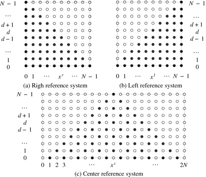
Figure 12.6 The search space: (xr, dr), (xl, dl), and (xc, dc): black and white dots represent, respectively, matching and occlusion nodes
The space occupied by the left and right reference systems consists of N × N nodes, where the number of matching and occlusion nodes is N(N + 1)/2 and N(N − 1)/2, respectively. In the center reference system, the nodes, (2N + 1)N, consist of N(N + 1)/2 matching nodes and N(3N + 1)/2 occlusion nodes. If the disparity range is limited to D < N, the space becomes the set of N × D and D(2N + 1) nodes, respectively. In designing the DP machine, the size of the space is a major factor because it correlates to the amount of space it consumes in the chip. Reducing D may therefore improve the space requirement significantly.
The given problem is to divide the space into two separate subspaces, above and below, so that the borderline becomes a disparity. The constraints are that the borderline must pass through the matching nodes – starting and ending nodes. The purpose of the DP algorithm (Aho et al. 1974; Bertsekas 2007; Cormen et al. 2001; Knuth 1997) is to find an optimal path along the x-axis. There are constraints associated with the optimal path. One constraint is that the path must travel through the matching nodes. The other constraint is the starting and ending nodes. In the right reference system, both ends must be (0, ·) and (N − 1, 0). In the left reference system, the two points must be (N − 1, ·) and (0, 0). In the center reference system, the extreme points must be (0, 0) and (2N, 0). Whether the path may go through the occlusion nodes is undetermined because there is no information on those nodes. The algorithm has the responsibility of deciding whether to include the occlusion nodes. The occlusion nodes may help to provide a smoother path but may also lead to wrong interpretation.
In both the left and right reference systems, it is expected that the matching result will become less reliable as the path progresses because the number of matching candidates will become smaller along the path. As a result, in the right reference system, the disparity is uncertain on the right side of the image. Likewise, in the left reference system, the disparity on the left end of the image is naturally uncertain. How the uncertainties are resolved depends on the algorithms, for example, by using the two types of disparity results. In the center reference system, there is no such bias depending on the direction of computation, except that the role of the starting and ending nodes can be changed, resulting in different disparity maps.
Finally, the left and right reference systems are not suitable for array design, although it is possible to use them. The data flow and the internal operations are very complicated. On the other hand, the center reference system is especially efficient when implemented in network arrays. In this chapter, we focus on single processor design, not array processor design, for the three reference systems.
12.4 Energy Equations
The next step is to define the energy function, defined on the search space, (x, d). In Chapter 6, we derived the energy equations for the three coordinate systems. To design the DP machines, we simplify the energy equations by including only the basic features and excluding higher order smoothness and occlusion constraints. However, more advanced energy functions can be applied to the DP machine by modifying the Verilog functions in later applications.
Consider a pair of epipolar lines, Il( ·, y) and Ir( ·, y). The corresponding energy equation in the right reference system is
where ρ( · ) is the local distance measure and μ( · ) is the smoothness constraint. Similarly, in the left reference system, the corresponding energy equation is
Here, the negative sign is used to retain the disparity nonnegative number. Finally, the center reference system has the energy equation
The major backbone of the DP machine is based on these underlying simplified energy equations. Higher-order terms and nonlinear time varying terms, which may appear in more specific algorithms, are all disregarded. Our purpose is to design a DP machine that is general in many ways – energy equation, DP algorithm, and architecture-so that more advanced terms can be easily imported later. Incorporating the advanced algorithms introduced in Chapter 6 is a challenging task. Even the distance measure for the local cost and smoothness will be defined in simplified forms.
12.5 DP Algorithm
Finding the optimal path that minimizes the energy equation can be conveniently explained with the connections between nodes in the search space, (x, d). For two nodes, (x − 1, d′) and (x, d), the connection has the configuration shown in Figure 12.7.
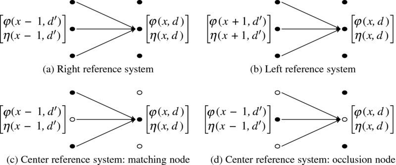
Figure 12.7 Paths from (x − 1, d′) to (x, d) in the three reference systems (only two neighbor nodes are shown)
As a part of the search space, (x, d), the horizontal axis denotes the computation direction and the vertical axis denotes the disparity levels. The direction in the left reference system is opposite to that of the right reference system. However, in the center reference system it does not matter because the search space is symmetric. In the center reference system, occlusion nodes are also included in the feasible paths for possible improvement of smoothness.
The concept is as follows. According to the previous computation, all the nodes, (x − 1, ·), already contain the cost, φ(x − 1, d′), and the pointer, η(x − 1, d′). In the current computation, (x, d) is resolved for the costs and pointers. For this purpose, (x, d) observes all the nodes in the previous column, (x − 1, ·), to choose the smallest cost and keep the node as a parent. In addition to the parent costs, some smoothness measure must be applied to the transition between the two nodes. The scope of parent search and the distance are often the major factors taken into consideration for smoothness. In the right and left reference systems, the transition is between two matching nodes, whereas in the center reference system it is between two types of nodes. There are four possible transitions: matching to matching, matching to occlusion, occlusion to matching, and occlusion to occlusion. In order to assign a suitable penalty to these transitions, we need to have some physical understanding of the geometry. Another observation is that the search range of the parent nodes can be limited to a small neighborhood. Smaller neighborhoods result in smoother disparities, even around object boundaries. Conversely, larger neighborhoods may result in noisy disparity distributions, although the disparities around object boundaries can be sharper.
From a computational point of view, choosing an optimal parent is a sequential operation, but the nodes, (x, ·), are all concurrent because they do not refer to each other for any costs or pointers. In the DP machine, we can realize this computation in either of two ways: the loop operation may need less space but run slower. The parallel realization is the opposite of the serial realization. It depends upon the conditions of the given resources. We will design the DP machine using many loops, which can be parallelized easily if required.
The DP algorithms must be defined separately for the three reference systems. For the right reference system in the space {(x, d)|x ∈ [0, N − 1], d ∈ [0, D − 1], the DP algorithm is as follows:
Algorithm 12.1 (DP algorithm for the right reference system) Given (Il( ·, y), Ir( ·, y)), determine {d(N − 1), …, d(0)}.
- Initialization: φ(0, d) = ρ(0, d), η(0, d) = 0, for d ∈ [0, D − 1].
- Forward pass: for x = 0, 1, …, N − 1 and d ∈ [0, D − 1],

- Finalization:
 .
. - Backward pass: for x = N − 2, …, 0,
The finalization is in fact trivial because the starting point is fixed, d(N − 1) = 0. However, this condition may be somewhat relaxed in a more advanced algorithm where other nodes (N − 1, ·) may be allowed as candidates for the starting node. The direction of computation is from x = 0 to x = N − 1 for the forward pass and from x = N − 1 to x = 0 for the backward pass. However, designing this algorithm in Verilog is not straightforward. The effect of the finite D, assignment of occlusion nodes with costs and pointers, signed and unsigned numbers, and overflow and word length, must all be taken into consideration.
The left reference system has a similar algorithm, but the coordinates are reversed.
Algorithm 12.2 (DP algorithm for the left reference system) Given (Il( ·, y), Ir( ·, y)), determine {d(0), …, d(N − 1)}.
- Initialization: φ(N − 1, d) = ρ(N − 1, d), η(N − 1, d) = 0, for d ∈ [0, D − 1].
- Forward pass: for x = N − 1, …, 1, 0 and d ∈ [0, D − 1],
- Finalization:

- Backward pass: for x = 1, …, N − 1,
The computation starts from x = N − 1 and arrives at x = 0 in the forward pass. Next, in the backward pass, the computation starts from x = 0 and ends at x = N − 1.
We have two options for combining the two algorithms. The first option is to keep the coordinates, xl and xr, in defining the costs and pointers. In this case, the computation proceeds in the direction of increasing xr (or decreasing xl), building the pointer array, ordered in the direction of increasing xr (or decreasing xl). The concept is intuitive but the shape of the search space and the pointer array are different in two coordinates system. The other choice is to define coordinates that increase in the direction of the forward pass. In this case, the structure of the pointer array is the same in both systems. We will use the latter option to design the DP machine.
Among the three coordinate systems, the algorithm structure of the center reference system is somewhat different from that of the others. Let us define the indicator functions: If x is even, ex = 1, otherwise, ex = 0. An odd indicator, ox, is therefore, ox = 1 − ex.
Algorithm 12.3 (DP algorithm for the center reference system) Given (Il( ·, y), Ir( ·, y)), determine {(x, d(x))|i ∈ [0, 2N], d ∈ [0, D − 1]}.
- Initialization: ρ(0, 0) = ρ(2N, 0) = 0, ρ(x, d) = ∞ for x − d ≤ 0 or x + d ≥ 2N.
- Forward pass: for x = 0, …, 2N, d ∈ [0, D − 1],
- for matching node (x + d = odd),
- for occlusion node (x + d = even),
- for matching node (x + d = odd),
- Finalization: d(2N) = 0.
- Backward pass: for k ∈ [0, D − 1],
- Map the disparity map:
In the initialization, nodes outside of the triangular zone in the (x, d) space are assigned very large numbers, which may prevent the optimal path from being in that region. The exceptions are nodes (0, 0) and (2N, 0), the start and end nodes of the optimal path. In the forward pass, node updating is carried according to the matching and occlusion nodes. There are four cases: matching to matching, matching to occlusion, occlusion to matching, and occlusion to occlusion. Different penalties can be assigned to the various different types of transitions. Parameters α and β denote the penalties for the occlusion nodes. The algorithm considers only three types of transitions. The backtracking is the same as that used in the right and left reference systems. As the pointers are retrieved, they must be mapped to the coordinates in the left or right image planes.
In order to allow for expansion to more advanced algorithms if needed, only the basic form of the DP algorithm is considered here. For example, more advanced algorithms may use features such as occlusion, neighborhood operations, and previous results.
12.6 Architecture
The concept of DP in Algorithm 9.1 is applied to stereo matching, as summarized in Algorithm 12.1. Let us design a circuit that implements this algorithm. One approach is to use a large state machine that computes everything from reading, processing, and writing. Let us use the processor that was developed as a component of the LVSIM – although we will modify it a great deal to accommodate stereo matching (see Chapter 4). The other parts in the simulator are all the same and thus need not to be repeated. Conceptually, the processor computes an image, line by line from top to bottom, and then outputs the result before the next raster line enters. In this section, we expand this structure more to facilitate the management of neighborhood operations and recursive computation.
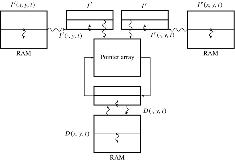
Figure 12.8 The concept of the Verilog DP machine
The major components of the DP machine are depicted in Figure 12.8. Three buffers function as the major data structure storing the intermediate data. Two buffers, called image buffers, store two rows of the images, left and right, that are read from the two external RAMs. The third buffer, called the disparity buffer, stores the previous disparity result read from the external RAM. The processor reads the images and the previous disparity results, computes the new disparities, and stores them in the disparity buffer. This computation progresses downwards in the image plane. For possible neighborhood operation, we expand the buffer to a set of rows, that is a strip. The buffers are actually FIFOs, in which the images enter the bottom and exit the top of the buffers. The three buffers are updated in synchrony. The objective is to update the contents of the center buffer with the corresponding images.
The machine computes the following mathematical equations:
where Il( ·, y) and Ir( ·, y) are the image rows, D( ·, y) is the desired disparity, and F( · ) is the main engine that computes the stereo matching algorithm. In addition to Il( ·, y) and Ir( ·, y), the computational structure allows us to use all the other components in the buffer, as a neighborhood. Further, the disparity buffer contains disparities, computed previously, in the current frame as well as the previous frame. The computational resources facilitate neighborhood and recursive operations, in addition to the primary algorithm, DP.
12.7 Overall Scheme
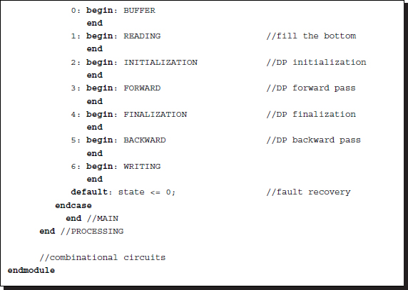
We design the system as a large state machine, with small sub-states within the big states. The required states are the buffer shift, reading, initialization, forward pass, finalization, backward pass, and writing states. Three states are associated with input and output, and four states with the DP algorithm. The states and their connections are illustrated by the state diagram depicted in Figure 12.9. The cycle starts from the buffer shift state. The three buffers, left image, right image, and disparity buffers, shift upwards, providing an empty line at the bottom. In the next state, the empty spaces are filled with the data from the external RAMs. Although the data at the bottom of the buffer are new, the data processed are those located along the center of the buffer. This arrangement is utilized in order to accommodate the possibility of neighborhood processing. The pixels along the buffer center can be grouped with their neighborhoods. The next state is DP computation, as specified in Algorithm 12.1. In the initialization state, the costs of the starting nodes are computed. The next state is the forward pass state, in which the costs and pointers are recursively computed and the pointers are written to the pointer matrix. When the forward pass ends at the final pixel position, the finalization process starts. Among the final nodes, the node with the minimum cost must be determined. In the three reference systems, this stage is trivial because the node with the minimum cost is already known. The backward pass process then starts, reading the pointers from the pointer matrix. When the process reaches the first pixel, it starts reading the next lines of images. For real-time processing, the computation in a loop must be completed within the raster scan interval.
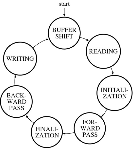
Figure 12.9 The state diagram of the DP machine
The DP machine must be designed for the three reference systems we have studied: left, right, and center reference systems. Designing separate machines may be very inefficient because they may have a great many parts in common, which will need to be modified later for specific applications. In Algorithms 12.1–12.3, the basic structures are all the same and thus must be retained in the code in the same way. Including common and difference codes in one package can be done using the Verilog compiler directives, `ifdef (Figure 12.10). With the header keys, LRC and LEFT, we can specify one of four modes: left, right, center left, and center right. In the left and right modes, the left and right image planes are the reference coordinate planes. In the center reference mode, the disparity obtained must be mapped to an actual plane, either the left or the right image plane, as derived in Equation (12.8). This requirement produces two more modes. In fact, there could be two additional modes in each of the center left and center right modes. In one mode, the computation proceeds from (0, 0) to (2N, 0) in the forward pass and returns in the backward pass. The other mode is the opposite – it proceeds from (2N, 0) to (0, 0) then reverses itself. The pointers retrieved in the two different ways are also different.
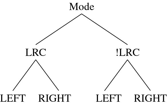
Figure 12.10 The three modes: left, right, and center (LRC) reference modes
Let us consider the overall framework of the DP machine. It has four main parts: header, variable declarations, procedural, and combinational.
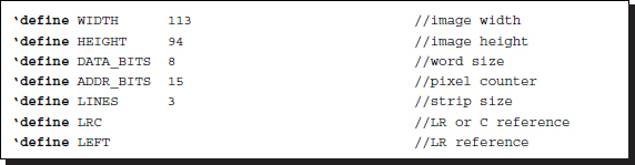
Listing 12.1 The Verilog DP machine: framework (1/7)
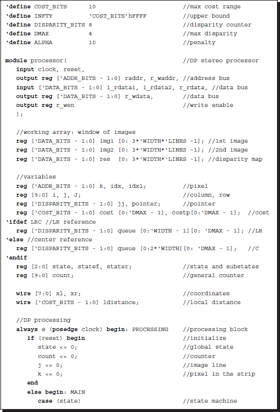
The header part assumes an image pair M × N in size, three channels, with each channel represented by a byte, and the total number of pixels specified. The three buffers are sub-images that have one or more lines of images. The parameters also define the reference systems – left, right, center left, and center right modes – using the keys LRC and LEFT. In addition, some constant numbers are defined, which we discuss below.
Inside the module keyword, ports are provided for interfacing with the three RAMs, a clock, and a reset signal. Two of the RAMs are for left and right images from cameras; the other is for the disparity result. In the variable declarations, the three buffers are defined as two-dimensional arrays. Three-dimensional arrays may be more natural for representing images but are more complicated to design. A two-dimensional array needs only one counter to access the contents, while a three-dimensional array needs two counters. The pitfall is that we have to consider the pixel coordinates in terms of the array order, which is rather complicated but advantageous for hardware implementation.
The procedural block consists of six states, as explained in the state diagram. The most important data structure is the queue that contains the pointers along the shortest paths. This table is filled during the forward pass and read from during the backward pass. It is an array of DMAX × N cells, where DMAX < N denotes the maximum disparity. The filled configuration follows that of the search space in the left, right, and center reference systems. If DMAX < N, the triangular region becomes trapezoid; the meaningful pointers are written inside this region. Outside the region, the pointers are meaningless and must be avoided by assigning high costs to them. The pointer array is huge, consisting of N × DMAX log DMAX elements, and thus the major bottleneck to the implementation. The final part is a combinational circuit that continuously monitors variables in the procedural block and computes required quantities, such as smoothness weight and local distance. This part largely depends on the applications and algorithms.
In the template, the combinational circuits are the same for all the reference systems. They also have parts in common inside the procedural block: reading and writing. The remaining parts are mixtures of common and dissimilar parts. In the following sections, we discuss in detail each of the components comprising the DP template.
12.8 FIFO Buffer
The first state of the DP machine is the buffer shift state. In this state, all three buffers shift one line upwards and leave the last line empty. The purpose of the FIFO buffer is to store the raster line and keep it stable during the disparity computation. Without the buffer, the same data would have to be read from the external RAMs, possibly many times, because the disparity computation may use the same pixel many times. The buffer could be just one line of image, but it is expanded to a set of lines in order to accommodate the possibility of neighborhood computation. Wider neighborhoods require more lines, but we typically use a four-neighborhood system, which means three lines of images. The basic goal is to use the centerlines from each of the three buffers to compute the disparity and store the result in the disparity buffer. If the local distance measure uses neighborhoods, then the image lines above and below the centerlines are also used. Each pixel also signifies three RGB channels, even for the disparity buffer.
To design such a buffer, we may use a circular buffer or just an ordinary buffer. In a circular buffer, the insertion point changes every time a raster line is to be written. In a shift buffer, the insertion point is fixed. We will use the shift register method (Figure 12.11).
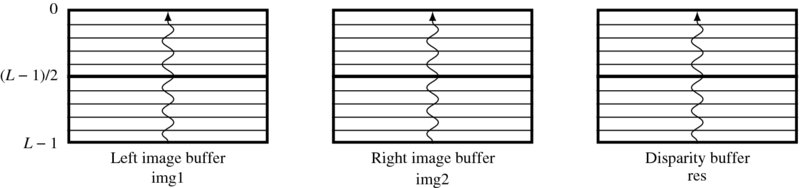
Figure 12.11 The operation of the three buffers: left image (Il), right image (Ir), and disparity (D)
As depicted in Figure 12.11, let us represent the three buffers by img1, img2, and res. The size of each buffer is L × 3N bytes, where L is the number of image lines and N is the image width. To make the coordinates symmetric above and below the centerline, L must be odd. The disparity computation is applied to the centerline, (L − 1)/2. The machine computes the following operations:
Here, T( · ) denotes disparity computation. In the array, the lines are numbered as [0, L − 1]. In this manner, the centerline is always the (L − 1)/2-th line, thus the neighborhood coordinates must be considered around it.
The pixel may appear in the image plane, buffer, and array and the exact coordinates must be calculated (Figure 12.12). The image plane is defined as {(x, y)|x ∈ [0, N − 1], y ∈ [0, M − 1]}. The buffer space is defined as {(a, b, c)|a ∈ [ − (L − 1)/2, (L − 1)/2], b ∈ [0, N − 1], c ∈ [0, 2]}. The corresponding array is {i|i ∈ [0, 3LN]}. If the origins are defined in each space as shown, a pixel appears at (x, y), representing column and row in the image plane – (a, b, c) in the buffer, representing row, column, and channel – and as (i) element in the array. A point (a, b, c) is mapped to i in the following way:
If the bottom of the buffer is written with the y′ image line, a point (a, b, c) is mapped to (x, y) in the following manner:
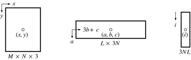
Figure 12.12 Three types of coordinates: image plane, buffer, and array
The transformation from buffer to array occurs often, so a dedicated function must be defined:
function ['ADDR_BITS - 1:0] id;
   input signed [9:0] row, column, channel;
begin
   id = 3*('WIDTH*((('LINES-1)>>1)+ row) +column) + channel;
end
endfunction
The shift operation of the buffer is as follows.
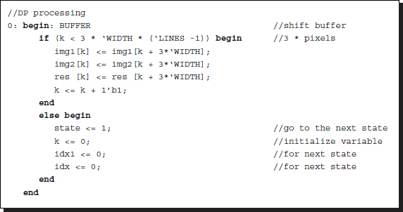
Listing 12.2 The Verilog DP machine: buffer (2/7)
This is the first state in the main code. The three buffers are updated concurrently. Because the buffer is represented by a two-dimensional array, only one counter is used here, at the cost of more involved coordinates. Two contiguous lines are separated by the distance, 3N, and thus shifting this amount is equivalent to shifting a row. Once the shift operation has been completed, the process moves to the next state, possibly by resetting variables. This stage uses 9NL space for three buffers and 3N(L − 1) time for shift operations.
12.9 Reading and Writing
The next state is provided for filling the bottom of the buffer. We are now involved with three external RAMs and three internal buffers. The three pieces of data must be read from the RAMs and written to the buffers, concurrently:
where Il, Ir, and D are the quantities in the external RAMs, respectively representing left, right, and disparity map.
The action used when writing is opposite to that used when reading. However, in this case, only the disparity buffer is stored. Because the most recent result is the centerline, it must be copied to the external RAM:
where J is the exact memory address defined by Equation (12.14).
The Verilog HDL code is as follows.
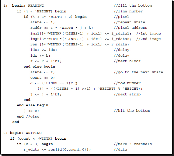
Listing 12.3 The Verilog DP machine: reading and writing (3/7)
Only one line must be read and the reading pauses until the large state loop is complete. Therefore, the line number and the center of the buffer must be kept in memory throughout the loop. This is explained in the buffer section. We have to be careful of delays that may be introduced between a piece of data and its corresponding address. This can be solved by using some auxiliary variables to store the previous addresses. The range of the loop must also be extended so that the address queue is emptied. Otherwise, the data in the last part of the loop may be lost.
In writing the state, the disparity buffer is written to the external RAM. Note that the disparity buffer is copied three times to make the three channels the same. The three RAM channels contain the same disparity map. This arrangement is necessary in order to provide grey level BMP files.
12.10 Initialization
The main part, Algorithm 12.1, starts at the initialization stage. The purpose of this stage is to provide two quantities: initial costs and pointers. For an M × N image, we consider the nodes defined in {(i, j)|i ∈ [0, N − 1], j ∈ [0, D − 1]}, where D is the maximum disparity, D ≤ N. For the right reference system, the costs are defined between Ir(0) and {Il(j)|j ∈ [0, D − 1]}. Therefore, the initial costs become
The three channels are treated separately. For the left reference system, the formula is somewhat different. The distance is defined between Il(0) and {Ir(j)|j ∈ [0, D − 1]}:
For the center reference system, the initial costs are
This condition holds whether the DP starts from (0, 0) or (2N, 0). A large number is necessary to mark all occlusion nodes apart from the starting node. The pointers can be anything, considering that the nodes have no parents at this point.
At this stage, the first column of the pointer matrix is filled, that is, {η(0, j)|j ∈ [0, D − 1]}. We use absolute distance measure for the three channels, but other measures can also be used.
The Verilog codes are as follows.
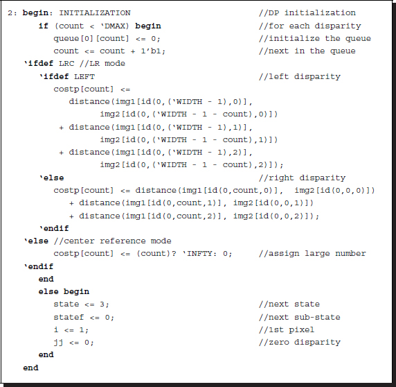
Listing 12.4 The Verilog DP machine: initialization (4/7)
Here, the distance measure is a function, which we will define later. In the distance measure, the coordinates of the buffer elements are rather complicated, due to the use of the Verilog array. The process is similar to that of delineating the two-dimensional image plane into a one-dimensional array. In calculating such coordinates, we have to take the image width and channels into account. Functions may simplify the coordinate transformation from the one-dimensional array to the two-dimensional array, and vice versa.
At the end of this process, there is a transition to the next state. The next state has both state and sub-states that must be clearly specified. In addition, variables, which will be used in the next state must be set to appropriate values. In this manner, we may reuse the same variables many times in different states, saving space but not the connections.
12.11 Forward Pass
The forward pass in Algorithm 12.1 comprises the core of DP. The key operation in this pass is the computation of cost and pointer for all the nodes. It provides a big table that stores the pointers. In the right reference system, the nodes are the elements in the space, {(xr, d)|xr ∈ [0, N − 1], d ∈ [0, D − 1]}. As a preliminary condition, the costs and pointers of the nodes, {(0, d)|d ∈ [0, D − 1]}, must have been determined in the previous initialization stage. The remaining nodes are subsequently visited and computed, recursively (Figure 12.13). In the figure, the horizontal axis signifies the number of pixels, while the vertical axis signifies the disparity. The maximum disparity level is denoted with thick lines. The arrows indicate the computing direction of the nodes in a column, and this is represented by a vertical line. In Figure 12.13(a), the search space is divided into two parts, inside and outside of the trapezoid. Inside the trapezoid, all the nodes are mapped to a pair of corresponding images. Outside the trapezoid, all the nodes are mapped only to the right image. In computing costs and pointers, the matching and occlusion nodes must be dealt with differently. The computation proceeds along the computing costs and pointers. The computation proceeds along the xr axis. The costs and pointers of the nodes at a point on the computing costs and pointers. The computation proceeds along the xr axis are computed using the costs and pointers of the nodes at the computing costs and pointers. The computation proceeds along the xr − 1 axis. The nodes on the same axis are all independent, allowing for possible parallel computation. For the occlusion nodes, the costs must be very large to prevent the optimal path from infiltrating this forbidden region. The pointers, which will never be used, may be arbitrary in this region. The result is the pointer array P = {η(x, d)|x ∈ [0, N − 1], d ∈ [0, D − 1]}, where x = xr.
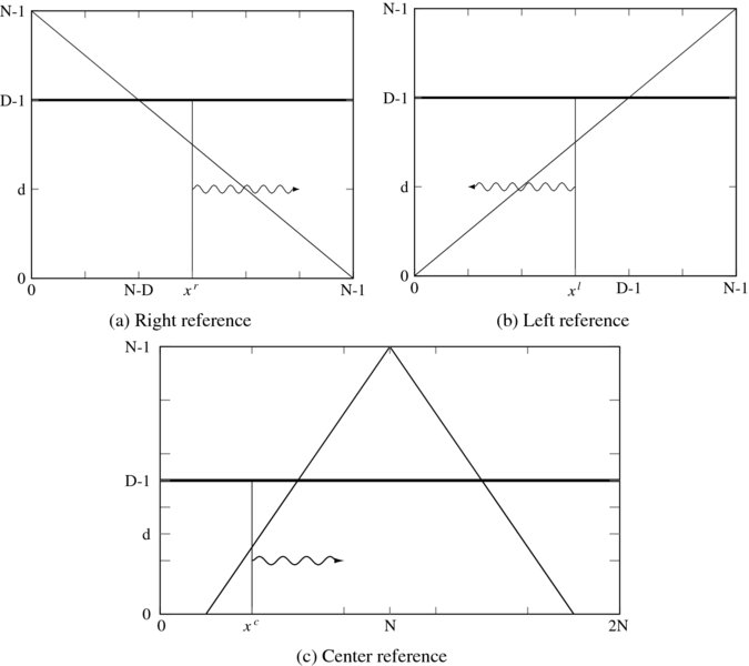
Figure 12.13 The (x, d) space: left/right and center reference systems
The left reference system has a similar interpretation. In Figure 12.13(b), the search space is S = {(xl, d)|xl ∈ [0, N − 1], d ∈ [0, D − 1]}. The shape of the trapezoid and the search direction are all opposite to those of the right reference system. The pointer array is also indexed in accordance with the direction of the forward path: P = {η(x, d)|x ∈ [0, N − 1], d ∈ [0, D − 1]}, where x = N − 1 − xl. This makes the pointer table the same type for both reference systems.
The forward pass operation for the center reference system is shown in Figure 12.13(c). The search space is S = {(xc, d)|xc ∈ [0, 2N], d ∈ [0, D − 1]} in this case. The shape of the search space is symmetric, and so the search direction can be either forward or backward, but the result obtained may be different. For the forward direction, the pointer table becomes P = {(xc, d)|xc ∈ [0, 2N], d ∈ [0, D − 1]}. The difficulty of this system is that the region inside the trapezoid also contains both matching and occlusion nodes (Figure 12.6(c)), which must be treated differently.
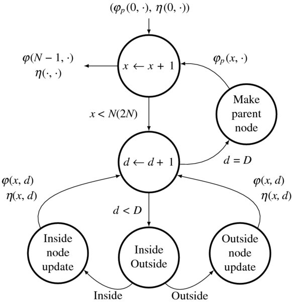
Figure 12.14 The computation of the forward pass: φ(x, d) and η(x, d) (the value in the parenthesis is for the center reference system)
In designing the forward pass, we first describe the algorithm with a state diagram (Figure 12.14). The diagram is common to both the right and left reference systems. The process starts at the initialization state, with φ(0, ·) and η(0, ·). The first state represents the big loop that computes in the direction of the column, x = 0, 1, …, N − 1. The second state represents the sub-loop that computes the rows, d = 0, 1, …, N − 1. In each of the rows in a given column, the node-pointer update is different, depending on whether the node is a matching or an occlusion node. For a matching node, the costs and the pointers are updated according to the DP equation. For an occlusion node, the cost must be given as an arbitrarily large number, which prevents the backtracking from passing the region over the diagonal. However, this assignment is not sufficient to prevent the optimal path infiltrating this forbidden region. A small addition to the large number may cause an overflow, resulting in a wrong number. For this reason, the positions inside and outside of the trapezoid must be considered in the node update.
For the center reference system, there are two differences in the flow graph. First, the column is limited to x ≤ 2N. Second, the nodes inside the trapezoid are not all matching nodes. The mixed matching and occlusion nodes inside the trapezoid must be dealt with differently.
Once all the nodes in a column are determined, the costs associated with the nodes present must be stored as the parent nodes, so that in the next column, the current column can be used as parent nodes. This series of computations completes one column and thus must proceed to the next column. When all the columns have been visited, the forward pass is complete, having φ(N − 1, ·) and η(N − 1, ·).
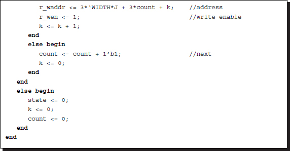
The concept in the diagram can be represented as the following Verilog code:
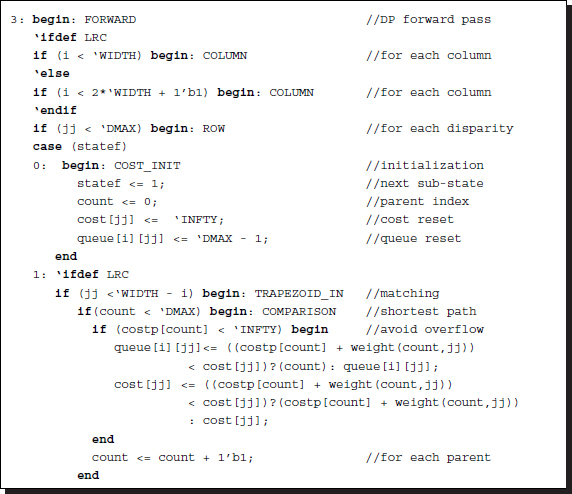
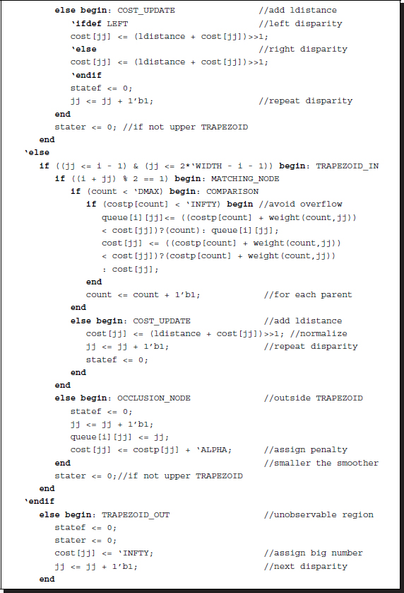
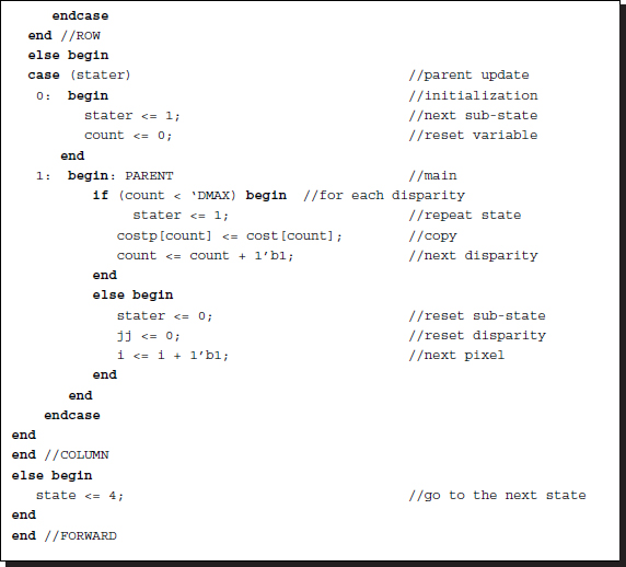
Listing 12.5 The Verilog DP machine: forward pass (5/7)
The forward pass consists of two loops (j and jj) as explained in the diagram. The internal loop (jj) is further divided into two parts: ROW_1 and ROW_2. The first part, ROW_1, is for updating node costs and pointers. The other part, ROW_2, is for collecting all the nodes and making them parent nodes. The two parts must be separated, otherwise the updated parents may be used too early in the current loop.
The node updating, ROW_1, also consists of two sub-parts: TRAPEZOID_IN and TRAPEZOID_OUT. One part is for updating the nodes inside the trapezoid; the other part is for updating the nodes outside the trapezoid. The state of the matching nodes inside the trapezoid also contains a loop, for comparing the costs of the possible parent nodes. In the center reference mode, the nodes inside the trapezoid are further divided into matching and occlusion nodes. All the conditions – matching to matching, occlusion to matching, matching to occlusion, and occlusion to occlusion – must be considered. In this code, the transition from occlusion to occlusion is excluded.
Note that, in computing local costs, there are transformations from buffer to image plane. Some parts of the code can be parallelized, whereas some other parts cannot be parallelized. The blocks, COST_INIT, COST_UPDATE, TRAPEZOID_OUT, and PARENT are possible candidates for parallelization. The block, TRAPEZOID_IN, however, is inherently serial. Note also that in COST_UPDATE, the cost update is significantly different among the reference systems and thus must be chosen appropriately by the compiler directives, `ifdef, `else, and `endif.
12.12 Backward Pass
In Algorithm 12.1, the finalization is the computation stage that follows the forward pass and appears before the backward pass. The purpose of this stage is to choose a starting point for the backward pass. The starting point must be a node whose cost is minimal among the nodes in the final column. In the three reference systems, this starting point is fixed to the last point of the triangle, making this stage almost trivial. For the left and right reference systems, the starting point is η(N − 1, 0), because the configuration of their pointer matrix is the same. However, the center reference system may start from either η(2N, 0) or η(0, 0).
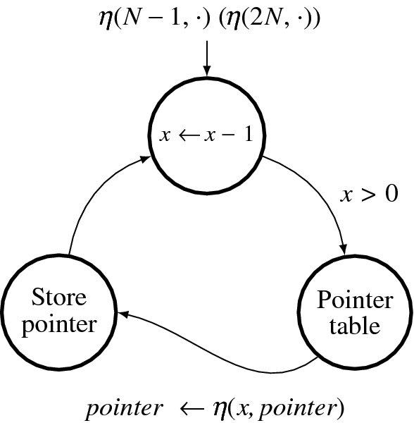
Figure 12.15 The backward pass (The expression in the parenthesis is for the center reference system. Others are for the left and right reference systems.)
The backward pass (illustrated in Figure 12.15) starts when the finalization state is complete. Starting from the end of the image pixel for the right reference system (reverse for the left reference system), the pointers in the pointer array are read in succession. For each reading, the pointer is written as a result on the disparity map. This concept is represented in the Verilog HDL as follows:
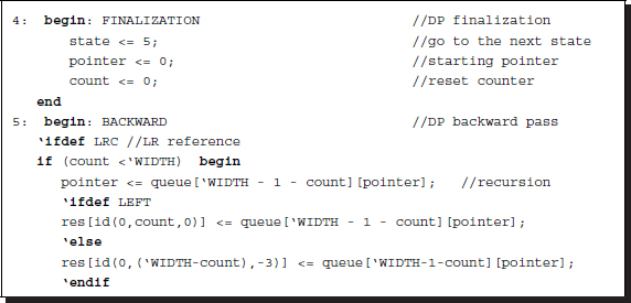
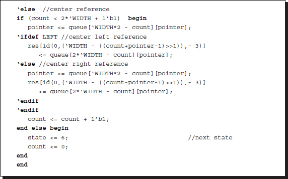
Listing 12.6 The Verilog DP machine: backward pass (6/7)
The disparity result is written to the first channel only. The two other channels are not used, but are instead reserved for other possible algorithms. Note that there are coordinate transformations from the buffer space to the image space. A combinational circuit is provided for monitoring the variables and providing the appropriate coordinate values.
In this code, the disparity map is exactly the same size as the image, including the three channels. The coordinates of the center reference system are also transformed to either the left or the right image plane. The disparity buffer and RAM can more than store the disparity. Usually D ≪ N, and so the three channels can more than represent the disparity range D, log 2D ≪ 24. This makes it possible to use the disparity buffer and RAM otherwise, that is to store information other than the disparity, such as features and other temporary results. We leave this possibility up to the actual applications that use the DP machine.
12.13 Combinational Circuits
The remaining parts are the combinational circuits and functions, which finish in the current simulation time. There are three parts: coordinates transform, weight computation, and local cost computation. The coordinates transform is for computing an array index from the given buffer coordinates, according to Equation (12.14). This can be easily realized by the Verilog function.
The cost computation needs two distance measures: smoothness measure and local distance measure. The smoothness measure is defined as an absolute of the two arguments:
The local distance measure uses the same absolute measure:
However, in the actual code, it becomes somewhat complicated because of the boundary effect, neighborhood computation, and the size of the strip. The use of neighborhoods can also be adopted in many different ways. Instead of the sum of individual differences, average features or edges may be used.
All three effects are considered in the following listing:
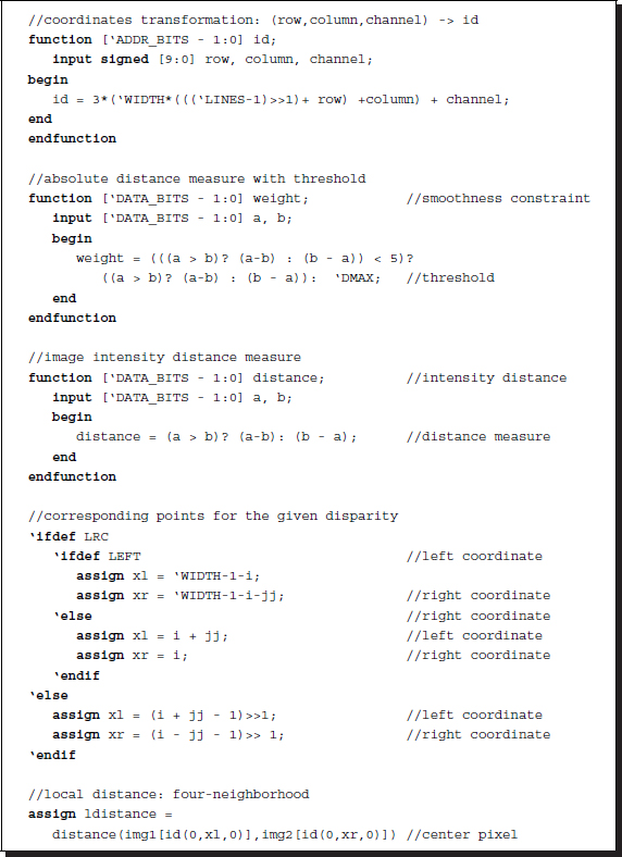
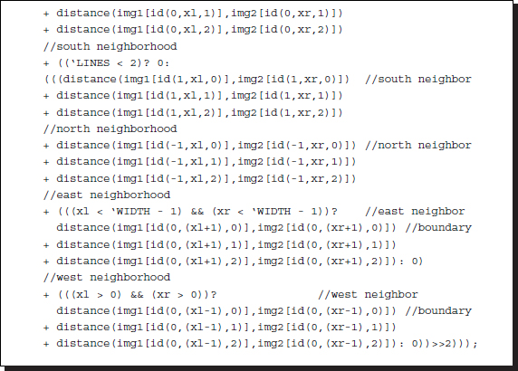
Listing 12.7 The Verilog DP machine: functions (7/7)
This template contains a local distance measure that uses four pixels from four-neighborhoods, together with the center pixel. To turn on the neighborhood computation, the buffer must contain at least three lines. Pixels beyond the boundary are assigned boundary values. However, mirror images or other types of boundary definitions may be adopted in this function. Moreover, even though the neighborhood is defined as a four-neighborhood system, it can be expanded to become a larger neighborhood system. All the neighborhood definitions are possible because the buffer has a general design for storing a strip instead of a single raster line. For better performance, the distance measure can be expanded to other measures such as Pott's model, edges, and features, instead of simple intensity values.
12.14 Simulation
We tested the code for both simulation and synthesis. There were numerous warning signals because we emphasized readability over optimization. However, before actual implementation, the code must be cleaned and optimized by rectifying as many of the warnings as possible.
The test images used were a pair of 225 × 188 images. The test images allowed us to test various versions of the DP machine. The first possibility was the reference modes: left reference, right reference, center reference right, and center reference left. The center reference has two modes, depending on where the disparity map is projected: left image or right image plane. In terms of the distance measures, there are numerous variations. The point operation and the neighborhood operations, in particular, must be compared for performance.
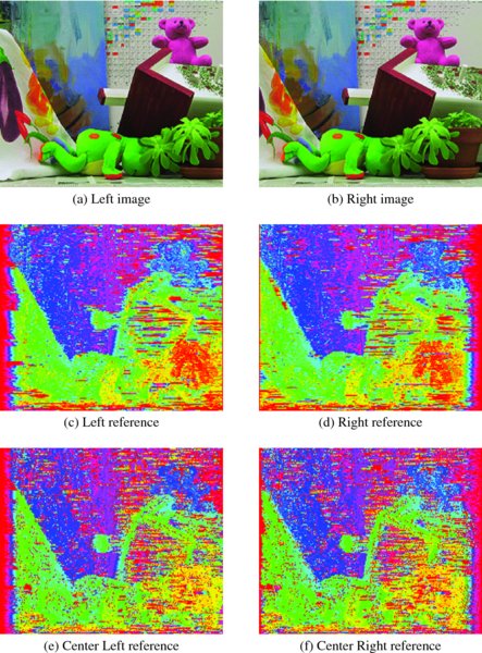
Figure 12.16 Disparity maps: point operations
The first sets of tests were point operations in the DP machine (Figure 12.16). Figures 12.16(a) and 12.16(b) are a pair of stereo images that have 225 × 188 pixels in three channels. The other images are the disparity maps obtained by the DP machine. The performance depends on the parameters and distance measures. As a first attempt, the disparity level, D, was restricted to 32, in order to observe the range of the disparity. The smoothness parameter was also limited to 5. The penalty from matching node to occlusion node was set to 10. In addition, the buffers contained only one line of images, which automatically turned off the local neighborhood operations, retaining only point operations. The original disparity map was a single channel gray map. For better rendering, the disparity map was made to three channels, histogram equalized, and color-coded. The result was a color map, with each level represented by a different color.
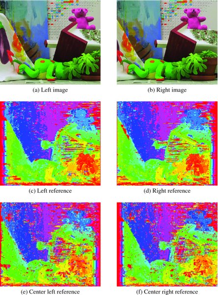
Figure 12.17 Disparity maps: four-neighborhood operations
Figure 12.17 depicts the simulation results. Three lines are used to compute local distance in a four-neighborhood system. The images in the second row (Figures 12.17(c) and 12.17(d)) are the disparity maps for the left and right reference systems, respectively. Of note is the fact that the left side is poor in the left reference and vice versa in the right reference. The disparity maps for the center reference are in the third row (Figures 12.17(e) and 12.17(f)). The disparity map is mapped to the left and right image planes.
A comparison of the two sets of simulations, that is point operation and neighborhood operation, easily shows the difference between them. The neighborhood operation provides a better disparity map but uses more combinational circuits and functions.
Because the purpose of designing the DP machine is to provide a standard template, it is generally configured with three buffers, which contain multiple lines, allowing possible neighborhood operations. Equally important, the reference systems are all counted in the design, which can be turned on and off by the header parameters. A simple condition on the transition between nodes is used in the center reference system. The size of the images and the level of disparities are defined by the parameters. As a result, advanced algorithms can be imported into this DP machine.
Problems
- 12.1 [Line processing] In a real-time system, the disparity for a line must be computed between the intervals of two successive lines. For an M × N pixel with a 30 fps video stream, what is the time interval between successive raster lines? How much time is allowed for each pixel?
- 12.2 [Computational space] In the right and left reference systems, if the disparity range is limited to D ≤ N, how many matching nodes and occlusion nodes are there?
- 12.3 [Computational space] In the center reference system, if the disparity range is limited to D ≤ N, how many matching nodes and occlusion nodes are there?
- 12.4 [Architecture] The three buffers are updated by shifting upwards and filling the bottom. What else could be done instead of shifting?
- 12.5 [Overall scheme] The DP machine was designed with a large state machine. How can you design it otherwise?
- 12.6 [FIFO buffer] The buffer is designed with the Verilog array. How can it be implemented using a Verilog multidimensional array? What are the advantages and disadvantages of the two methods?
- 12.7 [Reading and writing] In representing a line in the buffer, what is the equivalent representation for res[0,0,k], where
 ?
? - 12.8 [Forward pass] In the forward pass, the previous column is searched for all nodes, with the expectation that the occlusion nodes have a high cost. How can if (costp[count] < 'INFTY) be replaced otherwise?
- 12.9 [Forward pass] In choosing the smallest parent, the occlusion nodes are already assigned very high costs in the previous loop, and thus, adding a smoothness penalty does not allow them to be the parents. According to this observation, the conditions in the previous problem are not necessary. What is the problem in this method for treating all the nodes in the column the same way?
- 12.10 [Combinational circuits] What is the critical path that determines the fastest clock period?
References
- Aho A, Hopcroft J and Ullman J 1974 The Design and Analysis of Computer Algorithms. Addison-Wesley.
- Baker H and Binford T 1981 Depth from intensity and edge based stereo Proc. Seventh Int'l Joint Conf. Artificial Intelligence, pp. 631–636.
- Bertsekas DP 2007 Dynamic Programming and Optimal Control vol. 1,2. Athena Scientific.
- Cormen T, Rivest CLR and Stein C 2001 Introduction to Algorithms second edn. The MIT Press.
- Jeong H and Oh Y 2000 Trellis-based parallel stereo matching Proceedings of the IEEE International Conference on Acoustics, Speech, and Signal Processing, Istanbul, Turkey.
- Jeong H and Park S 2004 Generalized trellis stereo matching with systolic array Lecture Notes in Computer Science, vol. 3358, pp. 263–267.
- Jeong H and Yuns O 2000 Fast stereo matching using constraints in discrete space. IEICE Transactions on Information and Systems 83(7), 1592–1600.
- Jeong H, Oh Y, Park J, Koo B and Lee SW 2002 Vision-based adaptive and recursive tracking of unpaved roads. Pattern Recognition Letters 23(1), 73–82.
- Knuth D 1997 The Art of Computer Programming. Addison-Wesley.
- Ohta Y and Kanade T 1985 Stereo by intra- and inter-scanline search using dynamic programming. IEEE Trans. Pattern Anal. Mach. Intell. 7(2), 139–154.