
13
Systolic Array for Stereo Matching
In this chapter, following the single processor designed in Chapter 12, we design a systolic machine for stereo matching. Although the two machines are structurally different, they are both based on the line processing method (i.e. LVSIM) introduced in Chapter 4, which processes a frame line by line (or strip by strip), using small internal buffers. The systolic array introduced in Chapter 4 is a linear array consisting of many identical processors connected in a neighborhood fashion. This type of architecture is especially effective for VLSI implementation because it has many advantages, such as a regular structure, identical processors, neighborhood connections, and simple control.
This chapter first deals with the search space, because the problem is to find the path that incurs the least cost. We derive a systolic array, which is an efficient machine for such problems, in a systematic manner, following (Jeong 1984; Kung and Leiserson 1980; Leiserson and Saxe 1991). Using huge broadcasting, we spatially and temporally transform a simple circuit that matches the left and right image streams for disparity computation into the form of systolic arrays. The result is eight fundamental circuits that can be classified into two types: forward backward (FB), in which the two signal streams flow in opposite directions, and backward backward (BB), in which the two signals flow in the same direction. The multitude of circuits arises from the dualism or degree of freedom originating from the data direction, the head and tail, and the left right reference, resulting in the eight fundamental circuits.
We start designing FB and BB circuits, separately, as representative circuits, in Verilog HDL. The major components of the circuits are the systolic array, where actual computation is executed, and a control unit that drives the array. Although they look like datapath methods, both systems work in perfect synchrony with a common system clock, without any intervening handshake messages except for a starting signal, resulting in a very fast machine.
13.1 Search Space
For a pair of epipolar lines (Il( ·, y), Ir( ·, y)), the purpose of stereo matching is to find the disparity that exists in the space {(x, d)|x ∈ [0, N − 1], d ∈ [0, D − 1]}, for the left right reference systems, and {(x, d)|x ∈ [0, 2N − 2], d ∈ [0, D − 1]}, for the center reference system. The three types of spaces are shown in Figure 13.1. The measurable region is the trapezoids, a subset inside the rectangular region, formed by cutting the triangles. Areas out of this region are not observed by both cameras and are thus are indeterminate in nature. An object surface must appear as a line connecting (0, d) and (N − 1, 0) in the right reference, (0, 0) and (N − 1, d) in the left reference, and (1, 0) and (2N − 2, 0) in the center reference. For the three reference systems, the regions inside the trapezoid are defined by
Note that in the center reference, only the nodes that satisfy xc + d = even can be projected onto both images. In computing disparity, we use this equation as constraints on the search region.
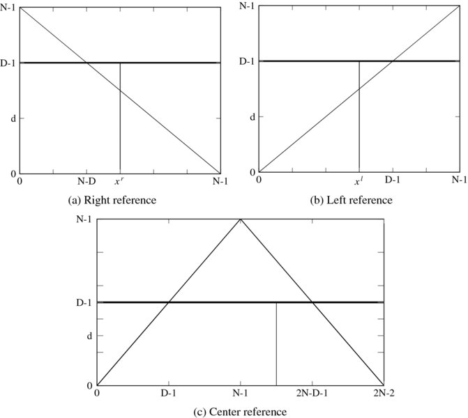
Figure 13.1 The (x, d) space: left, right, and center reference systems
In Chapter 12, we designed a DP machine that searches the solution space, column by column, as indicated by the vertical line. However, in this chapter, we present other methods for scanning the space, leading to the systolic array. We start the derivation of the array from a purely computational point of view below.
13.2 Systolic Transformation
We consider an array, {PE(d)|d ∈ [0, D − 1]}, where the processing elements are connected only between neighbors. In Chapter 3, we encountered a linear systolic array that computes convolution. In that system, the signal and the weights were the inputs, and the output was a weighted summation. The timing relationship between filter weights, the input signal, and the output was the key to the design of that array. Although seemingly different, the linear convolution and the disparity computation are, in fact, the same concept. The disparity is the result of the spatial relationship between two images. If the images are supplied by streams, the spatial relationship becomes the timing relationship. This transformation is possible by tilting the vertical scan line, as shall soon be seen.
Let us derive such an array in a more systematic way. The general idea is to begin with a simple circuit that we can easily understand; then we will modify the simple circuit to a more desirable form, following some intermediate stages. The techniques used in this approach consist of topological and timing transformation (Jeong 1984).
Before beginning, let us establish some data representation conventions. First, the image streams consist of the right and left images, Ir(t) and Il(t), where t ∈ [0, N − 1]. In the array circuit, the timing relationship between the two streams is the most important factor and we therefore consider only the sequence order. The order of the stream might be head first, I = 0, 1, …, N1, or tail first, I = N1, N2, …, 0, where Nx is an abbreviation for N − x. Second, the disparity is a nonnegative integer, satisfying
That is, in the right reference, the corresponding point in the left image is on the right of that in the right image. Conversely, in the left reference, the corresponding point in the right image is on the left of that in the left image. This property is essential in deriving the pipelined array with the two image streams, where the processing elements are numbered with disparities.
Let us first start with the right reference system. One of the simplest forms is a circuit in which the right image is broadcast to all the nodes and the left image is shifted into the nodes in a pipelined manner (Figure 13.2(a)). The numbered nodes denote the processing elements PE(d) with d ∈ [0, D − 1], where D = 3. The other two nodes are the hosts supplying the right and left images, as specified by the node labels. In this case, the image stream advances in head-first order. There are two things to note about the circuit. First, while the left image enters the array in its original order, the right image enters late, in the amount of D − 1 clocks. This delay is indicated by introducing ‘don't care’ in front of the right image stream. Note that this delay keeps the two streams synchronized correctly, in such a way that at PE(d), the right signal xr always encounters the left signal xl = xr + d.
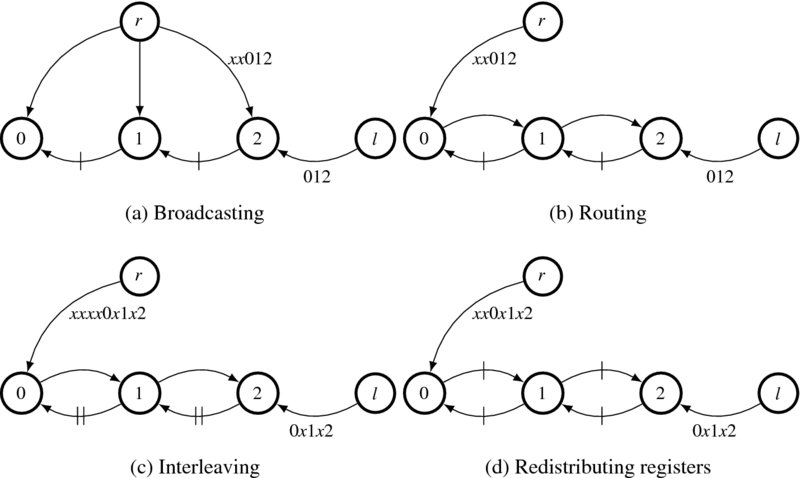
Figure 13.2 Deriving a systolic array, in which two image streams, Ir: xx012 and Il: 012, flow in the opposite direction (the edges are pipelined, and the leading ‘x’ denotes ‘don't care’)
Second, every edge between two nodes is blocked by a clocked register, although the edges from the two sources are free from this constraint. This small circuit with D = 3 operates as follows. After two clock periods, the two signals meet at the three nodes in pairs, PE(0): (Ir(0), Il(0)), PE(1): (Ir(0), Il(1)), and PE(2): (Ir(0), Il(2)). The relationship subsequently holds at all times, PE(0): (Ir(t), Il(t)), PE(1): (Ir(t), Il(t + 1)), and PE(2): (Ir(t), Il(t + 2)). Each node has only to compute the two incoming data streams for its disparity computation. In this dynamical system, the spatial relationship (xr, xr + d), is changed to the time relationship (t, t + d).
To describe the node behavior quantitatively, we use the notations Ii(d) and Io(d), respectively, for the input and output to a node PE(d). Consequently, node PE(d) performs the following.
where T( · ) denotes the operations for forward pass and y(d), the intermediate result.
This structure is very inefficient due to the broadcasting, which may be a major barrier to chip implementation. To remedy this situation, we have to modify the circuit topology so that the connection becomes regular and locally connected. Figure 13.2(b) depicts one way, among many, of delineating the topology (Jeong 1984). (There are numerous different ways. See the problems at the end of this chapter.) The three broadcasting edges from the right image source are reduced to one, while passing through all the nodes. To be an equivalent circuit, the node functions must be changed in such a way that an additional dummy input and output port that is internally connected to pass the input data to the output, is added to the node:
where the port Iro is added. This kind of node modification is trivial, and perfectly feasible.
The circuit topology is now regular, but the long combinational path still exists. We have to block all such paths with registers. However, we cannot arbitrarily insert registers or change the number of registers in the circuit because the timing relationship between data may be harmed. We have to consider using a pipelining technique, after examining the circuit topology. The point to note is that the circuit consists of three loops, each pipelined with a register. We need one more register to block the combinational path in the loop. One way to increase the number of registers without violating the circuit function is interleaving (or k-slow, in systolic terms). The penalty is that the circuit works at every other clock, slowed down twice, although the interleaved data can be used otherwise. (See the problems at the end of this chapter.) In Figure 13.2(c), the number of registers is doubled at all edges. Furthermore, the data streams, including the leading delays, are also interleaved. Check that the interleaved ‘don't care’ data, apart from preserving correct synchronization of the data streams, do not affect the computation on the normal data.
The next step is to redistribute the registers so that all the edges are pipelined. This task can be done by employing the retiming technique (Kung and Leiserson 1980). In Figure 13.2(d), the registers are redistributed correctly. In fact, the two leading ‘don't cares,’ which are equivalent to two register delays, are carried along the paths. The result is that the leading ‘don't cares’ are reduced by two and the registers along the broadcasting path are increased by two. Consequently, the critical path is reduced to the node delay, making the system very fast.
Incidentally, obtaining systolic arrays by topological and timing transformation has been studied in detail (Jeong 1984; Leiserson and Saxe 1991). Starting from a basic circuit, we can derive many functionally equivalent alternative arrays. The concept involves a combination of timing, spatial regularity, and duality. The circuit can be represented by an incidence matrix, whose elements represent vertex and edge registers. The topological and timing transformation can be represented by similarity transformations. In this chapter, we simply encapsulate the concept in an algorithm.
Algorithm 13.1 (Systolic transformation) Consider an array, {PE(k)|k ∈ [0, K − 1]}, having K nodes, all connected between neighbors only. The input streams are x(t) and y(t) for t ∈ [0, T − 1].
- Start from a basic circuit that has a large fan-out and a large fan-in. The node performs
where T( · ) is the internal operation and y is the intermediate result. The input streams are augmented by leading ‘don't cares,’ if necessary, to meet synchronization needs.

- Remove the fan-in and fan-out edges by routing them in one of many directions through the nodes. The node becomes

- If a loop consists of E edges and R registers, multiply all the edges by a constant ‘c’ so that
 and interleave the signals, including the leading delays, by c − 1 ‘don't cares’.
 - Redistribute the registers so that all the edges are blocked by at least one register.
- For dual circuits, repeat the process from the beginning.
In this formula, the broadcasting is generalized to the fan-in and fan-out, which are convenient for representing computation but inconvenient for circuit implementation. For the dual circuit, the following factors must be considered: the direction of routing, the signal directions, and the possibility of moving the three signals – input data and the result. It is potentially possible to make all the data move around the circuit, as evidenced by the circuits in Figure 3.10 in Chapter 3. With this concept as our basis, we will further derive the dual circuits.

Figure 13.3 Deriving a systolic array, in which two image streams flow in the same direction
13.3 Fundamental Systolic Arrays
Thus far, we have derived one type of systolic array, in which the image streams move in opposite directions. Intuitively, there must be another type of systolic array, one in which the two data streams move in the same direction. Let us derive this type of array using Algorithm 13.1. (Figure 13.3.) The starting graph is the same as before. In the second stage, however, the right image is routed in another direction and, as a result, the two streams flow in the same direction. In this circuit, there is no loop involved, so no interleaving is necessary. Consequently, pipelining can be easily achieved by supplying registers from the source side. Of course, the number of additional registers must be just enough to pipeline all the edges. Because there are two combinational edges, we need two additional registers. As such, two registers can be inserted in front of the sources, without violating data synchronization. (You may have to put in the lowest number of registers possible to save the registers and speed. In this case, the number is D − 1.) The inserted registers are moved along the paths and allotted to each edge in equal numbers (just one in this circuit). In addition, note that the transformation does not alter the overall function. Each node receives the input data in the correct order. The only change is the lead or lag between the host nodes and the arrays, which are not a problem from the viewpoint of the host. The result is that the edges on the upper path are pipelined with one register, while the edges on the lower path are pipelined with two registers. Like the original circuit, between the two paths, the time difference is preserved. In this manner, the upper stream moves twice as fast as the lower stream but must initially wait D − 1 clocks for correct synchronization. That is, the right image starts late but runs faster; the left image starts fast but runs slower. Because of this difference, four cases of time difference, which we call disparity, are possible. (We may call this circuit ‘tortoise and hare.’)
If duality is considered, many more circuits can be derived. In Figure 13.2, we assumed that the data are entering head first. The duality to this data order is that the data enter in tail-first order. Although there seems to be no benefit to this circuit, such a dual circuit actually exists. The basic circuit can be redrawn as depicted in Figure 13.4. As a perfect dual condition, no leading ‘don't care’ is needed at this time. As before, the broadcasting paths can be detoured in two directions. When the detour path is chosen as shown, the upper and lower paths are in the same direction. This circuit has no initial latency as in Figure 13.2, but has final latency. We must wait D − 1 clocks more for output depletion after the last set of data enters the circuit.
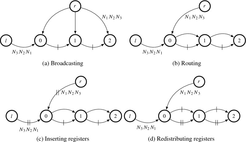
Figure 13.4 Dual to Figure 13.2. The data with bigger address (tail) comes first
The last dual circuit is obtained by detouring the broadcasting path in another direction. This is the dual circuit to Figure 13.3 Let us examine this circuit (Figure 13.5). When the right image is connected to the last node, the resulting path consists of loops. The newly introduced path contains no registers and must be blocked. To secure more registers in the loops, we rely on an interleaving technique. As in the previous examples, the number of registers is doubled and the input data streams are interleaved. The resulting circuit is equivalent to the original only at even periods. The registers are redistributed so that the combinational path is blocked. During this transformation, the input to the zero disparity must be delayed with D − 1 clocks, the number of edges along the upper path. The result is a pipelined circuit.
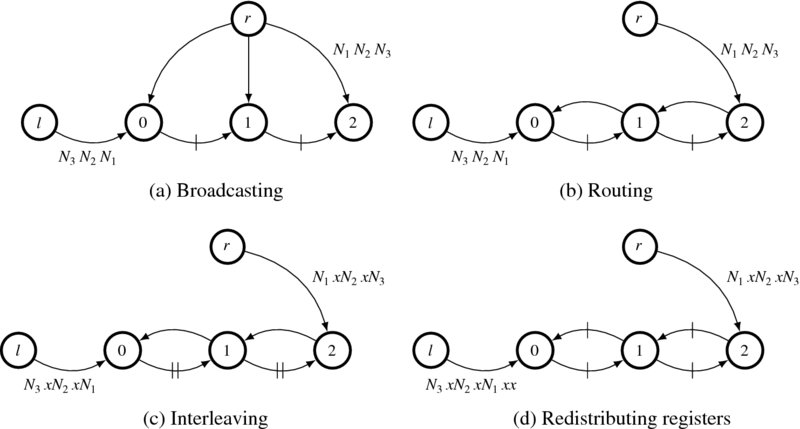
Figure 13.5 Dual to Figure 13.3. the data with bigger address (tail) come first
So far, we have derived four circuits for the right reference. If duality is considered, there must be four more equivalent circuits for the left reference, in which only the two streams are switched as inputs compared with the right reference system. Because there are so many circuits, we need a naming convention that differentiates them. One important factor is the direction of the streams, forward or backward, according to the array number. The other factor is the stream order, head or tail first. Yet another factor is the reference system, right or left reference. Combining these factors, we arrive at the eight circuits: FBR, FBL, BBR, BBL, FFR, FFL, BFR, and BFL, where F, B, R, and L represent, respectively, forward, backward, right, and left. They are in some way or another all dual to each other. Because many more circuits can be derived from these basic forms, we may call them fundamental circuits. All the circuits are listed in Figure 13.6. The first four circuits are interleaved and the others are not. The last four circuits need more registers, at the cost of original data ordering. All these circuits have different properties. The circuits are, in fact, all computing with the center reference system. Actually, the center reference is mapped to the right and left image coordinates, which we call center right and center left systems. Among the center left and right reference systems, FBR, FBL, BFR, and BFL are interleaved circuits. Circuits BBR and BBL have head-first streams but need initial delays, while circuits FFR and FFL do not need initial delays but need tail-first streams.
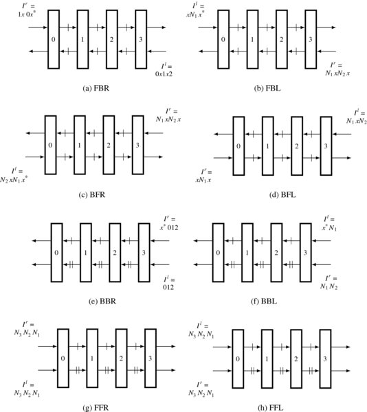
Figure 13.6 Eight fundamental systolic arrays for disparity computation (Na denotes N − a. x* denote D − 1 number of ‘don't cares’. In this case, D = 4)
According to Algorithm 13.1, there can be more equivalent circuits (see the problems at the end of this chapter). However, the eight fundamental circuits are the most efficient in terms of complexity and resource usage. Among the fundamental circuits, FBR is an identical circuit for center reference and has been extensively studied (Jeong and Oh 2000; Jeong and Yuns 2000; Jeong et al. 2002). In the following sections, we examine the properties of the fundamental circuits in more detail and choose the best candidates for circuit design.
13.4 Search Spaces of the Fundamental Systolic Arrays
We can compare the eight circuits by observing how they behave in the search space. Conceptually, the linear array is possible due to the slanted form of the scanning line, as opposed to the vertical line in Figure 13.1. This interpretation gives us an idea of the properties of the circuits as well as other possibilities (Figure 13.7). The solution space is defined by {(x, d)|x ∈ [0, N − 1]}. Depending on the reference system, the region of observation is determined, as indicated by the shaded area. A linear array corresponds to a line that scans the space. All the nodes in a line operate concurrently, finding their parent pointers and updating their costs. A node, PE(d), must access previous nodes, PE(d), PE(d + 1), and PE(d − 1), as shown, to determine a parent. The interleaved system, (a)–(d), corresponds to the circuits where the line slope is greater than one (empty circles are introduced between filled ones). In a scan line, two types of nodes operate alternately to match images. The remaining nodes must hold previous costs and pointers, in order to operate again when their turns come. The circuits with slope one, (e)–(h), do not need interleaving.
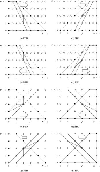
Figure 13.7 The relationship between computation and linear array in the left right reference systems. In this case, D = 5 and N = 6
Although all the eight circuits are valid, they are not all the same in terms of performance. The first factor affecting the performance is the starting points. Finding reliable parents heavily depends upon the costs of the parent nodes. In BF and FF, the computation proceeds in the space from fewer nodes to more nodes. On the other hand, in FB and BB, the computation proceeds in the opposite direction. Thus, the latter circuits will provide us with results that are more reliable. As a result, we will design circuits FBR (FBL) and BBR (BBL). The next factor is the form of the neighborhoods. In FBR, the parent candidates are (x, d − 1), (x − 1, d), (x − 1, d + 1). Among the nodes, (x − 1, d) must be stored in the previous scan line, where the corresponding node does not match anything but preserves the previous cost and pointer. The node (x, d − 1) means that paths through this node are all mapped to the same image point, which may give poor results. These properties hold for all the FB and BF type circuits. In BBR, no occlusion node is involved, so all the nodes are busy during the forward computation. There is one constraint that limits the performance, the parent (x, d + 1), along which all the points map to the same image point.
It is obvious that the scan line has two degrees of freedom – slope and direction – and thus results in various dual circuits. If the slope is infinite, the scan line is a vertical line. In such cases, the computation deviates from array, because one of the images must broadcast to the other every time the scan line moves. The serial algorithm in Chapter 12 was designed for such cases. If the slope is less than unity, the range of the neighborhood becomes large, deviating from the nearest neighborhoods.
13.5 Systolic Algorithm
Let us now build a systolic system and algorithm on the basis of the eight fundamental systolic arrays. In addition to forward processing, each processor must execute backward processing and other forms of processing. This means that additional ports need to be added to the fundamental circuits. Fortunately, these additional ports are the same for all of the fundamental circuits. In addition to passing image streams, the internal operations are all associated with maintenance of the pointer table. The required values are the costs from neighbor nodes and a bit, called the activation bit, denoting whether the neighbor node is on the shortest path. Because the communication is bidirectional, the number of input and output ports must be the same.
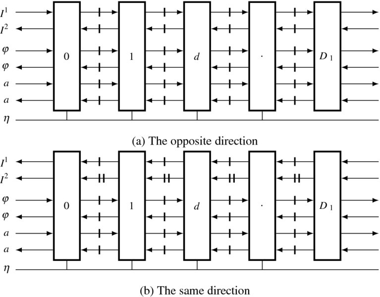
Figure 13.8 Complete form of fundamental systolic arrays for disparity computation (D1 means D − 1 for simplicity)
Considering all these facts, we can build two types of arrays, one type to perform forward processing and the other to perform backward processing (Figure 13.8). The array consists of the processors PE(k), where k ∈ [0, D − 1], and neighborhood connections among them. Although the registers are explicitly shown, they must be absorbed into the output ports of the processors. A PE has a pair of input and output ports for image, cost, and activity bits. Only the two end elements are connected outside as inputs. An output port may be directly connected to the input port or driven by the internal register. The pointer output is a two-bit line. All the outputs are connected by tri-state, driving a bus.
The two types of arrays can be further decomposed into two types of processors (Figure 13.9). In one type of processor, the directions of the image ports are opposed, while in the other, they are the same. When we build the algorithm, the controller must be described in terms of the arrays in Figure 13.8. The algorithm for the processor must be based on the two types of processors depicted in Figure 13.9. The following systolic algorithm must describe the internal operations of this basic element.
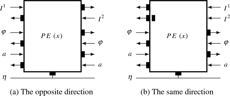
Figure 13.9 Two type of fundamental processing elements (the outputs ports are buffered by one or two registers)
In order to be a systolic system, the systolic array must be aided by a control unit. Therefore, unlike single processor algorithms, the array algorithm generally consists of two parts, one for the control unit and the other for a single processing element. While the control unit drives the array as a whole, feeding data and receiving the result, the processor only carries out its job on the entering data and outputs the results. The job of a processor can be recognized by its identification and clock counts, as a node is specified by (x, d) in the graph.
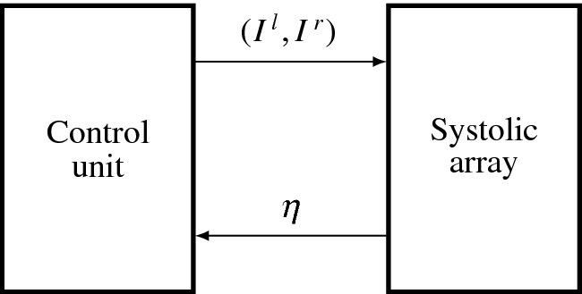
Figure 13.10 The systolic array system
The control unit and systolic array are connected as depicted in Figure 13.10. The systolic array is one of the two types shown in Figure 13.8. The control unit provides the image stream differently for each of the eight types of systolic arrays in Figure 13.6 and receives the output from all the array elements via a wired-OR bus. To avoid conflict, only one of the elements is allowed to emit the pointer, while the others are in tri-state or all zero. In this manner, the pointer can be obtained by bit reduction. The control mechanism is very simple because there is no handshake mechanism included between the control unit and the systolic array. After the controller initiates the systolic array, the two systems work independently but in synchrony with the common clock. Initially, the array element is in an idle state, waiting for the initiation signal from the controller. However, the controller needs more time than the array because it must do other jobs, such as updating the buffers, reading images from the RAMs into the buffers, and writing results back to the RAM.
Because there are eight types of systolic arrays, we have to write a general algorithm. Algorithms that are more detailed will follow in the later sections for particular circuits. As already explained, the algorithm consists of two parts: control unit and systolic element. The control unit performs the operations outlined in Algorithm 13.2.
Algorithm 13.1 (Control unit) Given (Ir, Il), do the following.
- Initialization: align the two image streams in the array.
- Forward pass: for t = 0, 1, …, N − 1, continue to feed the image stream.
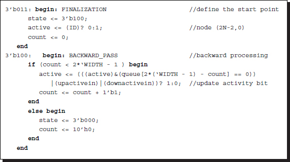
- Finalization: wait for the finalization, setting d(N) ← 0 (or d(0) ← 0).
- Backward pass: for t = N − 1, N − 2, …, 0, d(t) ← d(t + 1) + η(t).
The controller drives the systolic array, treating it like a black box. The purpose of the initialization is to make the array satisfy a state just one clock before the forward pass. This condition can be met by shifting the streams into the systolic array until the two streams fill all the registers but the last one. This condition is necessary because in the beginning of the forward pass, the first data of the two streams must meet at the last processor. The purpose of the forward pass is to feed the systolic array with the two streams in synchrony. After waiting a period for the systolic to finalize its operation, the controller starts to receive the disparity results from the systolic array. This value is differential, η ∈ {1, 0, −1}, instead of an absolute value and must therefore be accumulated. The initialization and forward pass depend on the eight types of circuits but the finalization and the backward pass are all the same. This is because all eight types of arrays use the same data structure for the pointers. It can be realized by an array or a queue. (See the problems at the end of this chapter.)
As a companion to the control unit, an element of the systolic array is executing a predetermined operation, as others, in synchronization with the system clock. The inputs are image, cost, and activity bit, while the outputs are image data, cost, and activity bit.
Algorithm 13.3 (Processing element) For a processor PE(d), do the following.
- Initialization: pass the image data.
- Forward pass: for t = 0, 1, …, N − 1, read φ(d + 1) and φ(d − 1), determine η, and update φ(d).
- Finalization: set a(0) ← 1.
- Backward pass: for t = N − 1, N − 2, …, 0, retrieve the pointer. If the active bit is true, set the activity bit of one of the two neighbor PEs, as indicated by the pointer and output the pointer. Otherwise, output high impedance.
The algorithm is designed for an individual element. All the elements carry out the same operation, in perfect synchrony. Each element knows its state by the two values, node ID, which is the disparity number, and the clock count, which is common to all. Once started by the controller, it operates itself up to the end of the backward pass, and then returns to the wait state. In the initialization state, an element simply passes the input image data in a predetermined number of times. In the end, its registers will all be filled with the image data. It subsequently enters forward pass, executing the predefined operations on the input images, passing the cost, and storing the pointer in its internal array. Finally, in the finalization stage, a particular element is set with its activity bit, which is predetermined as the node for disparity zero. The state then enters the backward pass, in which the pointer array is read, one of the two neighbors are set or reset with the activity bits, and the pointer is issued. The pointer output may be disabled by tri-state if it is not an active node.
The difficulty of the systolic array design lies in the preparation of the initial condition and the correct synchronism in the data streams. Once synchronized perfectly, the system becomes a very fast circuit, with no more intervening control messages. To cover the eight fundamental circuits in a compact code, we have to make as many common constructs as possible. To design the circuit, let us first consider the hardware platform that is commonly used for all types of circuits.
13.6 Common Platform of the Circuits
The basic structure of the systolic machine is analogous to the LVSIM but varies somewhat, as shown in Figure 13.11. (Compare this with Figure 12.8.) Three buffers are the major data structures storing the intermediate data. Two buffers, called the image buffers, store two rows of the images, left and right, that are read from the two external RAMs. The difference is that these buffers are expanded with more channels so that feature vectors can be stored too. The third buffer, called the disparity buffer, stores the new disparity, updated in this period or the previous disparity result, read from the external RAM. The three buffers are arrays with a three-dimensional structure in column (x), row (y), and channel (z), following the image, I(x, y, z), where z signifies the channel. We usually store RGB in the first three channels and the feature maps in the remaining channels. However, the number of channels may vary from one to multiple channels, depending on the application. In addition to the expanded channels of the image buffers, one more component is added – the systolic array.
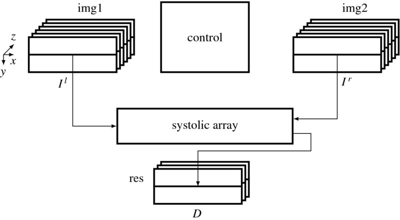
Figure 13.11 The concept of the systolic systolic machine. The three buffers, img1, img2, and res, respectively, store Il, Ir, and D, and the control unit controls the buffers and the systolic array
With the four major resources, the processor executes the following operations, supervised by the control unit. First, the processor reads the images and the previous disparity results, into the three buffers. It then processes the images in the buffers (i.e. RGB channels in img1 and img2) and stores the features in the remaining channels of the two buffers (i.e. channels 3, 4, 5, or 6 in img1 and img2). The control unit constructs two streams of feature vectors out of the two image buffers and feeds them to the systolic array as inputs. In the end, as the array emits a stream of disparity values, the control unit stores them in the disparity buffer. The control unit returns to the beginning and repeats the same series of operations. In this manner, the computation proceeds downwards for a pair of epipolar lines in the image frames.
For possible neighborhood operation, we expand the buffer to a set of rows, that is strip instead of a line of an image. The buffers are actually FIFOs, in which the images enter the bottom and leave the top of the buffers. The three buffers are updated in synchrony. In this manner, the three buffers indicate the same window of the image frame at all times. For the added preprocessing, the image buffers contain more than three channels to store the feature maps. The intention is to update the contents of the buffer center with the corresponding images.
Mathematically, the machine computes the following equations:
where Il( ·, y) and Ir( ·, y) are the image rows, including feature vectors, D( ·, y) is the desired disparity, and T( · ) signifies the main operations of the stereo matching algorithm. In addition to Il( ·, y) and Ir( ·, y), the computational structure may enable us to use all the other components in the buffer, as a neighborhood. Moreover, the disparity buffer contains disparities, computed previously, in the current frame as well as the previous frame. The computational resources enable us to conduct preprocessing, neighborhood, and recursive operations, in addition to the primary algorithm, DP.
In the following sections, this system is used as a platform for the design of FB and BB circuits.
13.7 Forward Backward and Right Left Algorithm
The first choice of the eight fundamental circuits is the FB system, which is characterized by the right reference and the image streams moving in opposite directions. As dual circuits, FBR and FBL are the same except for the fact that the roles of their two inputs are reversed. As a result, we can explain the algorithm primarily in terms of FBR. The architecture of the FBR system is shown in Figure 13.12. Initially, the left image shifts down the array to fill all the buffers but the last one. Subsequently, the right image also enters the array, first meeting the left image at PE(0). During the forward pass, the cost ports, φ, are active. The state then enters the backward pass, in which state the activity ports, a, are active. The results drive the bus so that the output reaches the controller. As boundary conditions, the input ports at the end processors must be terminated with suitable values. In this case, the terminal conditions are φ = ∞ and a = 0. The processors use the same values as the others, executing the same operations as the others, and avoiding complicated logic for testing boundary conditions.

Figure 13.12 The FBR system (x* denotes D − 1 ‘don't cares’. Each out port is buffered by one register. The input terminals are fixed with φ = ∞ and a = 0.)
The search space and circuits are not enough to define a detailed algorithm. We need the most detailed description, the timing diagram. This diagram may provide the precise operations of the controller and the array element on the basis of clock ticks. Let us return to FBR in Figure 13.7(a). The figure describes the search space, (x, d), and the computational order. By following the activities of the elements, we can build a new space, (t, d), which we may call a timing diagram (Figure 13.13). The horizontal axis is the time and the vertical axis is the disparity. In actuality, the graph, (t, d), is an affine transformation of (x, d), in which the originally slanted scan line is erected into the vertical direction. Further, this space is equivalent to that of the center reference. In the forward pass, the computation proceeds as indicated, and the direction is reversed in the backward pass. The nodes on the computation line try to match images for the costs and pointers or retain the previous costs and pointers, depending on the costs being compared. The result is the pointer table, (η, t). A possible solution may be the lines from ‘A’ to ‘B’, which can be traced during the backtracking. Note that the start point is fixed but the end point may be any point on the left side of the trapezoid.

Figure 13.13 The computational space, (t, d), of FBR. In this case, D = 5 and N = 6. The dashed line is a possible solution
The algorithm must respect the trapezoid region and its boundary. The region is an affine transform of that in the (x, d) space (refer to Figure 13.2(a)). For both FBR and FBL, the trapezoid is defined by
The spaces (x, d) and (t, d) have the following relationship:

where t is again equivalent to the center reference coordinates.
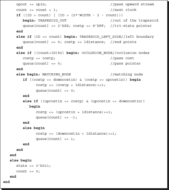
Each processor must know where it is located in the space, especially in terms of the trapezoid. In the forward pass, a processor is in one of the four states: out of the right side, on the left side, out of the left side, matching node inside the trapezoid, and occlusion node in the trapezoid. The region located out of the right side is the forbidden region and thus all the nodes there are assigned tri-state for the pointer and a very large number for the cost. The tri-state logic allows us to bundle the outputs from D processors into a line. (See the problems at the end of this chapter. The tri-state output can be used for a wired-OR gate. The other alternative is logic zero; in which case, we can use bit reduction.) The high cost simplifies the comparison in the event of parent decision. Even the boundary processors – PE(D − 1) and PE(0) – are arranged to receive very high costs from their pseudo-neighbors. The nodes along the left side are all the same points on the right image. They must be treated specially because they must be the end of the shortest path. Beyond this side, the nodes are visited in the backtracking but should not change the disparity value, which has already been determined on the left side. This policy needs to be implemented using some technique during coding. Inside the trapezoid, the matching node is the major place where the pointer and cost must be determined on the bases of neighbor costs and input images. The comparison can be done without worrying about the boundary conditions because illegal nodes have already been assigned very large numbers in the previous stages. The occlusion nodes do no matching but play the role of keeping cost and point to the previous matching node. The role of the node alternates between matching and occlusion as we move along the timeline.
In the backtracking, node (2N − 2, 0), is the only starting node. There is only one starting node but there are D possible end nodes, all located on the left side. The pointers must be compact, indicating relative positions to the parents with three possible values, ( − 1, 0, 1). The true disparity is the accumulated value of the pointers. After recovering the shortest path, the positions must be mapped to the right image, in accordance with Equation (13.7).
Let us now formally describe the algorithm. To denote the connecting ports, we use the subscripts ‘i’ and ‘o’ for input and output ports, respectively, and ‘u’ and ‘d’ for upper and lower PE, respectively, keeping in mind the structure, Figure 13.8.
Algorithm 13.4 (FBR: control) Given Ir = {Ir(0), x, Ir(1), ⋅⋅⋅, Ir(N − 1)} and Il = {Il(0), x, Il(1), x, …, Il(N − 1)}, do the following.
- Initialization: for t = 0, 1, …, D − 2, Ili(D − 1) ← Il(t).
- Forward pass: for t = 0, 1, …, 2N − 2, Iri ← Ir(t) and Ili ← Il(t + D − 2).
- Finalization: d(2N − 2) ← 0.
- Backward pass: for t = 2N − 2, 2N − 3, …, 0,
The system is interleaved and thus twice the image width is needed for the clock period. As a result, the length of the pointer array is 2N − 1. In the initialization state, the left image flows into the array, filling the D − 1 registers. In the forward pass, there is an offset, D − 2, between the left and right image streams. After the end of the left image stream, the flow continues with D − 2 more values, which may be arbitrary. During the backward pass, the pointers are accumulated but sampled at even periods only.
All PE(d), d ∈ [0, D − 1], do the same operations. For convenience, let us use an indicator function, I(x) = 1 if x ≠ 0 and I(x) = 0 if x = 0.
Algorithm 13.5 (FBR: processing element) For a processor PE(d), do the following.
- Initialization: for t = 0, 1, …, D − 2, Iro ← Iri and Ilo ← Ili.
- Forward pass: for t = 0, 1, …, 2N − 2, do the following.
- Iro ← Iri, Ilo ← Ili, φuo ← φ, and φdo ← φ.
- If d > t or d > 2N − 2 − t, then η ← 0 and φ ← ∞. else if d = t, η(0) ← 0, then φ ← |Iri − Ili|, else if t + d = even,
else, η(t) ← 0 and φ ← φ.
- Finalization: a ← I(d = 0).
- Backward pass: for t = 2N − 2, 2N − 4, …, 0,

In the initialization phase, PE(d) with d ≠ 0 is also assigned η = 0. This simplifies the logic during the backward pass operation. During that period, all PEs issue η to the bus. Among them, only one PE issues the desired pointer, the others do not. However, all the outputs are connected together, making a bus. Therefore, the output of the unactivated PE must be zero (wired-OR) or tri-state (bus). We prefer the former method, due to its simplicity. In the forward pass, η ∈ {1, 0, −1} represents one of the three parents, PE(d + 1), PE(d), and PE(d − 1). The search region is within the trapezoid, R in Equation (13.6). A unmatched node within the trapezoid simply retains its previous cost and zero pointer.
For the FBL, Ir and Il are reversed in their roles and switched for their ports in the controller. However, the systolic array is exactly the same. The algorithm describes the overall scheme but still misses some details that are possible only in the actual coding. The following section explains the overall framework of the Verilog HDL code.
13.8 FBR and FBL Overall Scheme
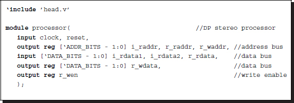
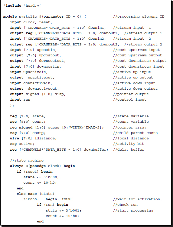
The specifications of the circuits can be defined by a header file, head.v.
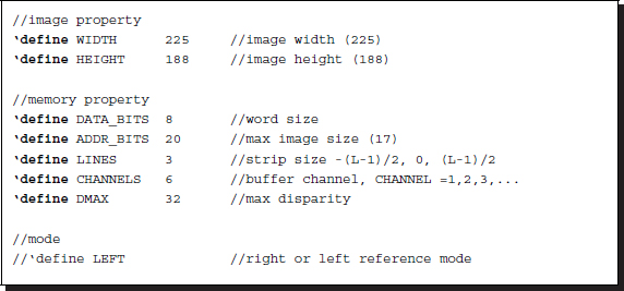
Listing 13.1 The framework: head.v
With the header keys, LEFT, we can specify one of the two modes: FBR and FBL. All the image and disparity specs are defined by an M × N image, three buffers with L lines, and the disparity level D. There can be one or more channels. One channel may signify mono, while additional channels may signify RGB colors or feature maps. The maximum disparity level is D < N.
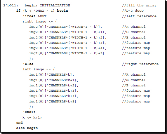
Next, for the main part, we design the system with two subsystems, one for the control, Algorithm 13.4, and the other for the systolic element, Algorithm 13.4. However, the control contains additional tasks, in addition to the systolic control, such as buffer management, reading, and writing. The states and their connections are illustrated by the state diagram in Figure 13.14. The system starts from buffer shift for the control and from the waiting state for the array. The three buffers, left image, right image, and disparity buffers, shift upwards, providing an empty line at the bottom of each buffer. In the next state, the empty lines are filled with the data from the external RAMs. Although the data on the bottom of the buffer are new, the data to be processed are located along the center of the buffer. The philosophy underlying this arrangement is facilitation of the possibility of neighborhood processing. In this scheme, the pixels along the buffer center can be grouped with their neighborhoods. The two systems are completely synchronized only in the DP computation – initialization, forward pass, finalization, and backward pass and decoupled during the other periods. This synchronization is activated by a semaphore, which invokes the idling processors. In the initialization state, the costs of the starting nodes are computed. The following state is the forward pass, which recursively computes the costs and pointers, and writes the pointers into the pointer matrix. When the forward pass ends at the final pixel position, the finalization process starts. Among the final nodes, a node with the minimum cost must be determined. In BF circuits, this stage is the most trivial because the node with the minimum cost is already known. From there on, the backward pass starts, reading the pointers from the pointer matrix. When the computations hit the endpoint, they restart and read the next lines of images. For real-time processing, the computation in a loop must be completed within the raster scan interval.
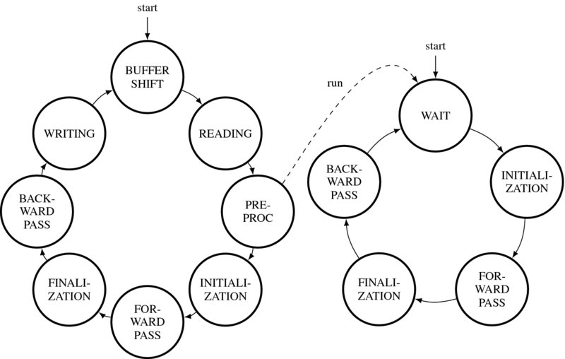
Figure 13.14 The state diagrams of the controller and the systolic array. The controller activates the systolic array and synchronizes itself up until the end of backward pass
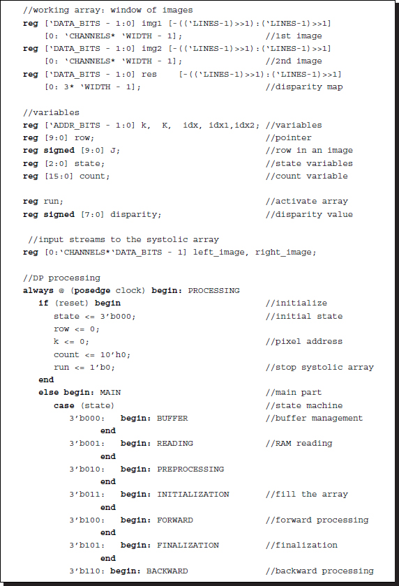
The code, processor.v, is used to realize the control unit, Algorithm 13.4. Let us look at the overall control framework, in which the states are removed and labeled instead.
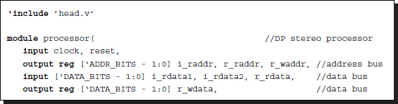
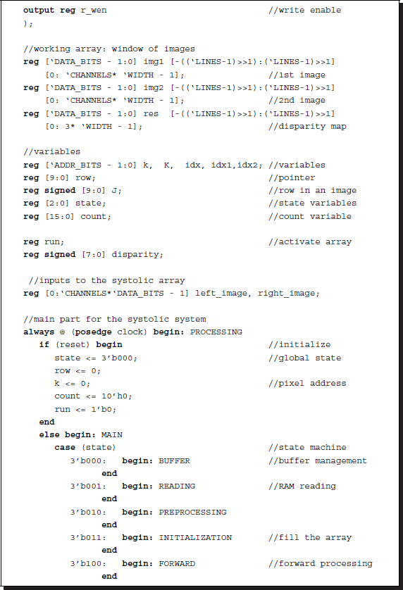
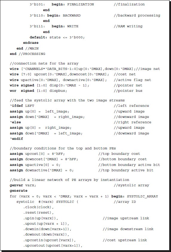
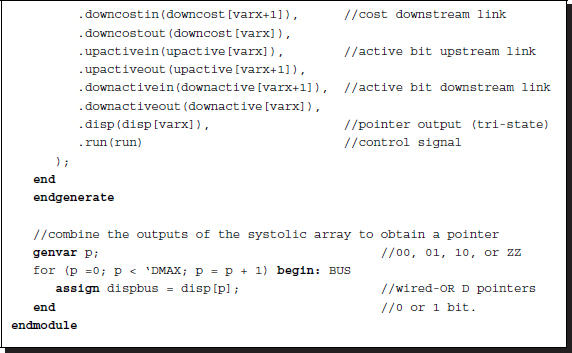
Listing 13.2 The framework: processor.v
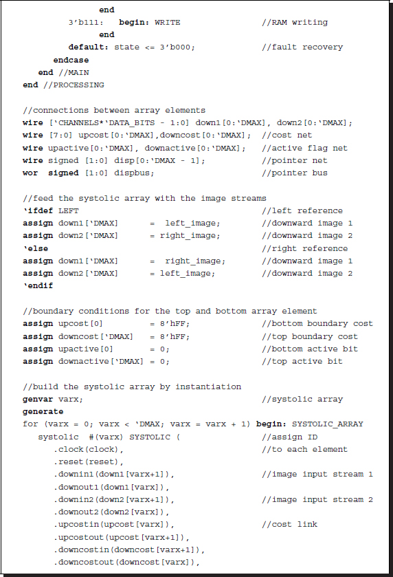
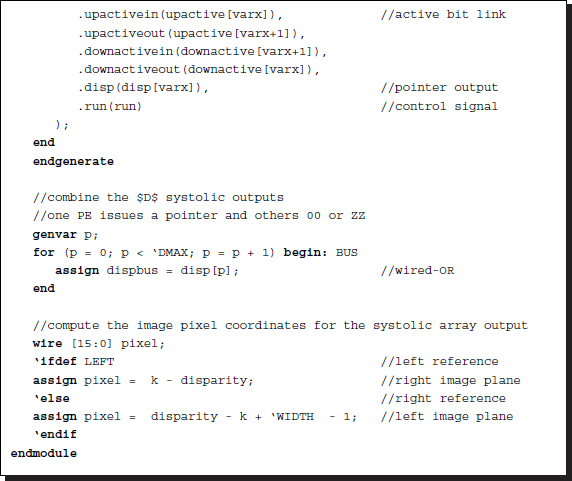
Conceptually, the code realizes Algorithm 13.4. It consists of four parts: a procedural block, instantiation, input, and output. The code instantiates the systolic array, SYSTOLIC, linking individual processing elements to net arrays. Through the links, the streams of images (Il and Ir), cost (φ), and activation bits (a) flow upwards and downwards, so that an element can receive the necessary data from both neighbors and send the processed data to both neighbors. Note also that the processors located at the top and bottom of the array are missing in one of the two neighbors. The streams from the missing neighbors must be provided appropriately: φ = ∞ and a = 0. The terminal processor can then execute the same neighborhood operations as the others. The control also plays the role of driver, supplying the array with two image streams, in both directions. In FBR, the upstream is the right image and the downstream is the left image. In FBL, the roles of the two images are reversed. Finally, the output is the pointers from the array. Among the D elements, only one emits a valid pointer, a two-bit binary, while the others emit tri-states or zero. To detect the valid pointer, we can combine the output lines via wired-OR. (See the problems at the end of this chapter.)
The code for the processing element, systolic.v, realizes Algorithm 13.5. This code is instantiated by the control to form an array, consisting of D elements. Each element executes the same operations, depending only on the time and processor ID. The ID is assigned by the instantiation and the time is known by the synchronized clock. No more handshaking is needed, sparing unnecessary communication overhead. The system behaves like an engine, where all the operations are already predetermined by the clock and processor identification.
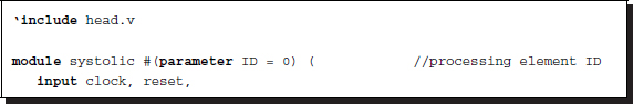
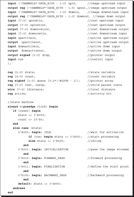
Listing 13.3 The framework: systolic.v
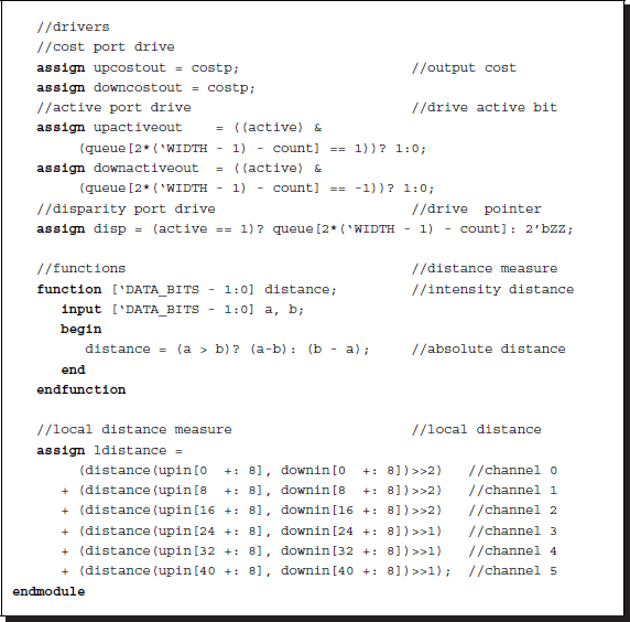
The code consists of four parts: a procedural block, driver, and cost computation parts. The procedural block is a companion to that of the control unit and thus will be explained shortly together as a pair. The purpose of the processor is to send the correct output to the output ports after undergoing internal operations. The values to be sent to the output ports are the costs and the activation bits. Next, for internal operation, local cost is needed in updating parent costs. This computation is realized with the combinational circuit, which takes the two image data, computes the distance between them and supplies it to the forward pass operation. The template shows a basic example, in which all the six channels are used to compute the distance measure. In terms of the distance measure and the combination of channels, schemes that are more elaborate must be adopted for better performance.
Now let us examine the parts of this system one by one in more detail.
13.9 FBR and FBL FIFO Buffer
The first state of the systolic machine is the buffer management. In this state, all the three buffers shift upwards just one line and leave the last line empty. The purpose of the FIFO buffer is to store the raster line and keep it stable during the disparity computation. Without the buffer, the same data must be read from the external RAMs, possibly many times, because the disparity computation may use the same pixel many times. The buffer could be just one line of an image or a set of lines. In the latter case, neighborhood computation is possible. The neighborhood operation needs more than one line, typically three lines for the four-neighborhood scenario. The three buffers are the windows, mapping the same positions of the image plane. The basic goal is to update the centerline of the disparity buffer, using all the other buffers. Because the position of the image that corresponds to the buffer center is changing, it is required that that position be remembered in order to write the result back to the memory later. If the local distance measure uses neighborhoods, then the image lines above and below the centerlines are also used (Figure 13.15).
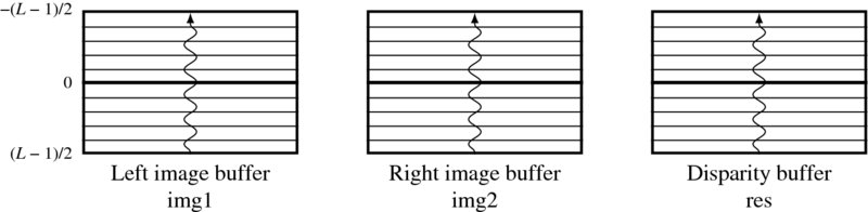
Figure 13.15 The three buffers: left image, right image, and disparity buffers
We may use a circular buffer or just an ordinary buffer in the design of such a buffer. For the circular buffer, the insertion position changes every time a raster line is to be written. In the shift buffer, the insertion position is fixed. We will follow the shift register method. The system contains three buffers, one for the left image, one for the right image, and one for the disparity. The left right image buffers have dimension, L × N × C, characterized by the number of lines, L, and channels, C. The image buffers have more channels than required for the input images. The extra channels are used to store the features' vectors obtained after preprocessing. Conversely, the disparity buffer has a smaller number of channels, just enough to store the disparity map.
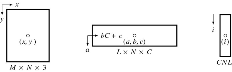
Figure 13.16 Three types of coordinates: image plane, buffer, and array
To code the buffers, we need to define the coordinates for the pixels in the buffers. The underlying concept is that the array is numbered [ − (L − 1)/2, (L − 1)/2], instead of [0, L]. This is done so as to always make the centerline the origin and thereby the neighborhood pixels can be easily located. Consequently, a pixel appears with different coordinates in image, buffer, and array. We have to know the exact relationship among the coordinates (Figure 13.16). The image plane is defined as {(x, y)|x ∈ [0, N − 1], y ∈ [0, M − 1]}. The buffer space is defined as {(a, b, c)|a ∈ [ − (L − 1)/2, (L − 1)/2], b ∈ [0, N − 1], c ∈ [0, C − 1]}. The corresponding Verilog array is {i|i ∈ [0, CLN − 1]}. If the origins are defined in each space as shown, a pixel appears as (x, y), meaning column and row in the image plane, (a, b, c) in the buffer, meaning row, column, and channel, and as (i) element in the array. A point (a, b, c) is mapped to i in the following way:
If the bottom of the buffer is written just with y′ image lines, a point (a, b, c) is mapped to (x, y) in the following manner:
The modulo arithmetic is necessary to manipulate the case when the raster line is located at the bottom of the image. The transform from buffer to RAM is needed whenever the disparity map is to be written to the external RAM.
The shift operation of the buffer is as follows:
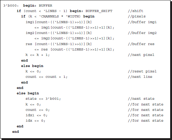
Listing 13.4 Buffer: processor.v
This is the first state in the main code. Three buffers are updated concurrently. Because the buffer is represented by a three-dimensional array, in the sense of the Verilog array, two counters are used here, rewarded by the easy coordinates. (See the problems at the end of this chapter.) Two contiguous lines are separated by the distance, CN, and thus shifting this amount is equivalent to shifting a row. Once the shift operation has been completed, the operation moves to the next state, possibly by resetting variables. This stage uses (2C + 3)NL space for three buffers and CN(L − 1) time. If the buffer contains a line, no time is consumed here. For larger buffers, this part may take the longest time of all and thus must be optimized by using dedicated buffers, or altered by directly reading from RAM, although some of the functionality of the system may inevitably be lost.
13.10 FBR and FBL Reading and Writing
The next state is provided for filling the bottom of the buffer. We are now involved with three external RAMs and three internal buffers. The three sets of data must be read from the RAMs and written to the buffers, concurrently. The writing action is opposite to that of reading. However, in this case, only the disparity buffer is stored. Because the most recent result is the centerline, it must be copied to the external RAM.
The code reads as follows:

Listing 13.5 Reading and writing: processor.v
The reading is somewhat involved because the RAM and the buffer has a different number of channels. While a pixel is assigned three channels in RAM, the same pixel is represented by more than three channels in the buffer. The read data must be written to the first three channels in each pixel.
This state reads a line and then stops until the whole loop is completed. Therefore, the line number and the center of the buffer must be kept, throughout the loop. Two unit delays are introduced between an item of data and the corresponding address. In the loop end, the range is extended so that the address queue may be emptied and thus the data in the last part of the loop may not be lost.
The last state is reserved for writing, in which the disparity buffer is written to the external RAM. The same contents of the disparity buffer is written into three channels, to make a gray level bitmap.
13.11 FBR and FBL Preprocessing
After the buffers are loaded, we can conduct preprocessing to extract features or filtering. In the image buffers, the first three channels contain the source images in RGB format. The other channels, if available, are provided for storing features. The preprocessing stage is a template provided for processing the image channels and filling the feature channels. A basic example is to average vertically to obtain feature vectors.
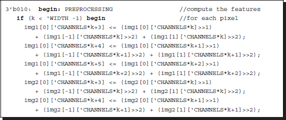
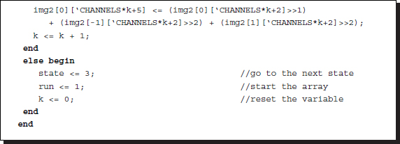
Listing 13.6 Preprocessing: processor.v
If the neighborhood operation is to be extended to the four neighbors, boundary conditions must be considered, as in Listing 4.17. Note that, due to the new definition of the coordinates, the neighborhood pixels can be easily located.
If the incoming image is black and white, the number of channels is just one or greater. If preprocessing is needed, an additional channel may be added to store the feature map. In an actual system, this part must be elaborated in such a way that the feature maps may affect the distance measure and the good disparity result.
Up to this state, the controller does not yet invoke the systolic array. As soon as the preprocessing is finished, a control signal, that is, ‘run,’ must be sent to the array, preemptively one clock before, so that from the next initialization state, both control and systolic array can be synchronized.
13.12 FBR and FBL Initialization
From this state to the end of the backtracking, the control and the systolic array execute concurrently in perfect synchrony. Therefore, the two systems must be explained together. According to Algorithms 13.4 and 13.5, the control supplies one stream of images and the array fills itself with the stream. Through D − 1 clocks, D − 2 registers must be filled because, in the next state, the two streams must meet head to head in FBR (tail to tail in FBL) at PE(0).
The control unit must build two streams of feature vectors, out of the image buffers, and possibly with the disparity buffer and supply them on both terminals of the array.
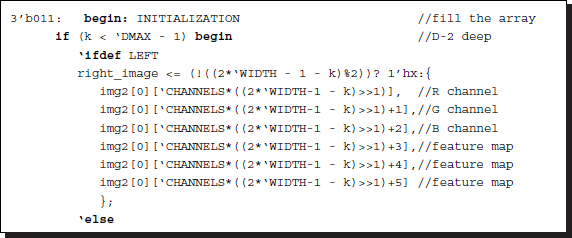
Listing 13.7 Initialization: processor.v
In FBR, the left image flows down the array just before the bottom array, before the right image enters. In FBL, the right image flows down while the left image is waiting. The difficulty is that the two streams must be interleaved.
On the array side, the state is idle and waiting for the semaphore from the control unit. As soon as this bit enters, the state changes to the initialization process:

Listing 13.8 Initialization: systolic.v
In this instance, the control and array are in perfect synchrony. Each processor passes the downstream for the predetermined number of times: D − 2.
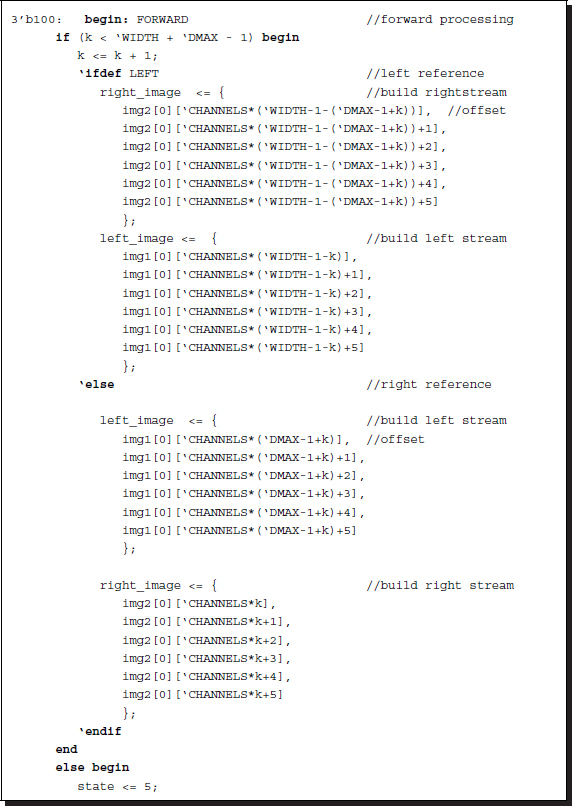
13.13 FBR and FBL Forward Pass
The forward pass in Algorithms 13.4 and 13.5 is the core of DP. In this state, the control continues to supply the image streams and the array while passing the streams, and computes the required operations, through 2N − 1 clocks. The key operation is the computation of the cost and pointer for each processor, providing a 2N − 1 long pointer array.
The control is relatively simple because the operation is simply to supply the data stream.
Listing 13.9 Forward pass: processor.v
The stream must be a smooth continuation from that of initialization. Complications arise, however, from the combined effect of the left right mode, the interleaving, and the even and odd D. As a result, the four cases shown arise. The control unit packs two image streams with the buffer contents and supplies them in the predefined order to the systolic array.
The purpose of the array element in the forward pass is twofold: buffering two image streams and determining a pointer and a cost value.
Listing 13.10 Forward pass: systolic.v
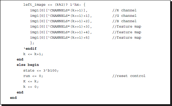
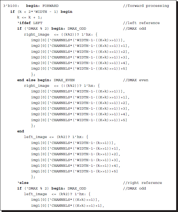
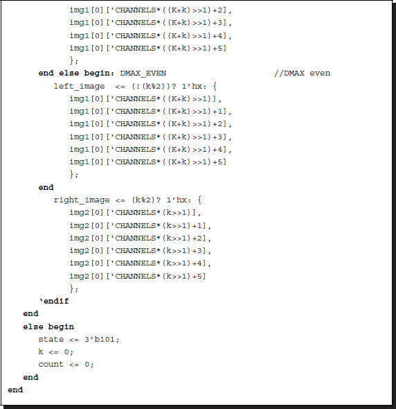
The details of the task depend on where the element is located in (t, d) space. There are four possibilities. The first possibility is that the position is located out of the right side of the trapezoid. In that case, the cost is assigned a large number and the pointer is arbitrarily assigned, because it will never be accessed. The second possibility is that the position is on the left side of the trapezoid, which is the end position in the backtracking. Therefore, the cost and pointer are assigned a local cost and zero pointer, respectively. Beyond the left side, the cost that was determined already in the previous endpoint must be maintained until the loop ends. Inside the trapezoid, the position might be an occlusion, in which case the cost and pointer must be retained until it becomes a matching node in the next clock. (A node alternates between matching and occlusion.) Otherwise, it is the matching node and must be computed using the normal Viterbi method. The basic operation is to compare the neighbor costs and decide on a parent. The pointer is an incremental disparity, relative to the current node. This operation is the same for the terminal elements in the bottom or top of the array because those processors are terminated with very high costs, which prevent the possible shortest path intervening in those positions.
As shown in Listing 13.3, the local cost is computed with the image inputs by the combinational circuit. There are many variations on the cost computation and weights on the neighborhood.
13.14 FBR and FBL Backward Pass
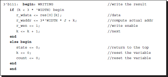
In Algorithms 13.4 and 13.5, the finalization is the computation stage that follows the forward pass; it appears before the backward pass. The purpose of this stage is to choose a starting point for the backward pass. The starting point must be a node whose cost is minimal among the nodes in the final column. In FBR and FBL, this point is fixed to the last point of the triangle, making this stage almost trivial. However, there are D candidate points in BFR and BFL, necessitating a full finalization process. As such, the starting point is PE(0), which means the first pointer, η = 0.
In the control side, this concept is represented in Verilog HDL as follows:

Listing 13.11 Backward pass: processor.v
In the backward block, the control receives the pointer via a wired-OR network. Among the D pointers, only one is valid and the others are tri-states. The values are signed and thus accumulation gives the disparity. This computation is done by the combinational circuit in Listing 13.2. One of the complicated parts is the ending points along the left side of the trapezoid. The other part is the assignment of the disparity to the correct pixel.
In the systolic array side, the role is to provide the control circuit with the pointer, driving a port with a combinational circuit, as shown in Listing 13.3. The code for the systolic array is as follows.
Listing 13.12 Backward pass: systolic.v
Setting and resetting a one-bit flag, called the activation bit, is the key point in the operation. In the finalization, the processor sets or resets its activation bit depending on whether its ID is d = 0. The combination of the activation bit and the output of the pointer array create various cases. As such, the activation bit is set or reset depending on the combined states. The pointer is output to the bus when its activation bit is set. Otherwise, the output is a tri-state, which has no effect on the wired nets.
13.15 FBR and FBL Simulation
For simplicity, we did not correct the codes for numerous warnings. Most of the warning signals were for the number casting from long to short word length. After checking whether the codes were synthesizable, we observed the outputs.
As before, the test images were a pair of 225 × 188 images. With these test images, we could test FBR and FBL. The purpose of the simulation was to check the correctness of the code, not to optimize the performance by applying advanced techniques, which are unclear and dependent on applications.
The starting point was the circuit with point operations (Figure 13.17). The top figures are a pair of stereo images, having 225 × 188 pixels in three channels. The remaining images are the disparity maps obtained by the systolic machines. The performance varied depending on the parameters and distance measures. As one of the parameters, the disparity level, D was restricted to a value of 32, observing the range of the disparity. No other parameters, such as smoothness, were adopted in the coding. For point operation, the buffers were allowed to contain only one line of images, which automatically turned off the local neighborhood operations. The original disparity map was a single channel gray map; however, for better rendering, it was expanded to three channels, histogram equalized, and color-coded. The result was a color map, with different levels represented by difference color.
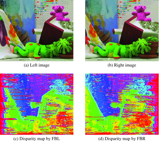
Figure 13.17 Disparity maps: point operations (D = 32)
Figure 13.18 depicts another set of simulation results. Three lines were used in computing local distance in the four-neighborhood scenario. The images in the second row are the disparity maps for left reference and right reference, respectively. Note that the left side is poor in the left reference, and vice versa.
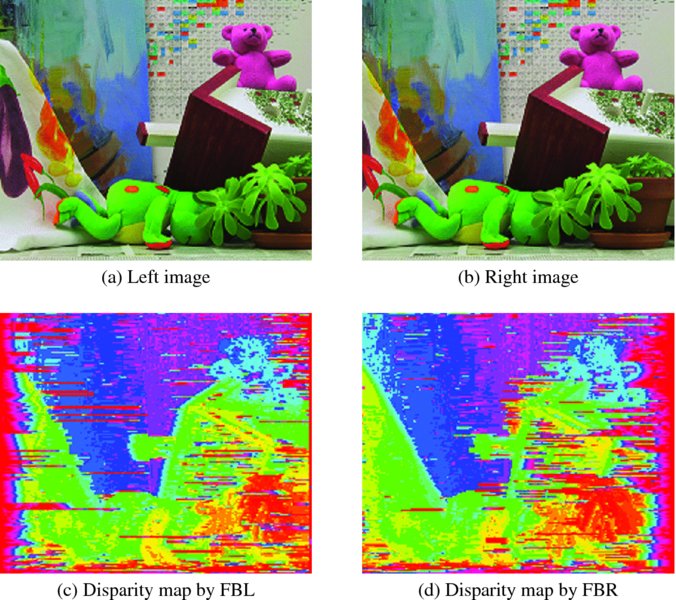
Figure 13.18 Disparity maps: four-neighborhood operations (D = 32)
A comparison of the two sets of simulations – point operation and neighborhood operation – easily shows the difference. The neighborhood operation provides a better disparity map but uses more combinational circuits and functions.
Because the systolic machine is being designed in order to provide a standard template, it is generally configured with three buffers, containing multiple lines, which allow for possible neighborhood operations. Of equal importance is the fact that the reference systems are all counted in the design, which can be turned on and off by the header parameters. A simple condition on the transition between nodes is used in the center reference system. The size of the images and the level of disparities are defined by the parameters. As a result, advanced algorithms can be imported into this systolic machine.
13.16 Backward Backward and Right Left Algorithm
Of the eight fundamental systolic arrays, the second type is the arrays, BBR, BBL, FFR, and FFL, in which the two image streams flow in the same direction (Figure 13.6). With the exception of their flow directions and data ordering (head or data first), they are all equivalent. The BBR (and thus BBL) is the most natural choice for a design because it features right reference and head-first data direction. Let us proceed to the design of BBR and BBL.
The architecture of the BBR system is illustrated in Figure 13.19. Initially, while the left image shifts down the array to fill all the buffers, the right image waits at PE(0). Subsequently, the two flows meet and enter the forward pass. During this state, the cost ports, φ, are actively used to transfer costs between neighbor processors. After the input streams are exhausted, the state enters the backward pass, in which the activity ports, a, are activated to trace the processor along the shortest path. The results of all the processors drive the same bus so that the output reaches the controller. The input ports located on both ends of the array must be terminated with suitable values, φ = ∞ and a = 0, which are analogous to boundary conditions. The end processors use these values and the values from others to execute the same operations as others, free from testing boundary conditions, which make the computation very complicated.
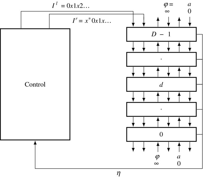
Figure 13.19 The BBR system (x* denotes D − 1 ‘don't cares’. Each out port is buffered by one or two registers. The input terminals are fixed with φ = ∞ and a = 0.)
In order to design the system, it is essential that the algorithm be understood at the level of events. That is, the exact tasks carried out by the controller and the array element in each clock tick have to be known. Let us observe BBR in Figure 13.7(a). The figure describes the search space, (x, d), and the computational order. Following the activities of the elements, we can build the space, (t, d), as shown in Figure 13.20. The diagram shows the disparities computed and their respective times. In the forward pass, the computation proceeds to the right, building pointers. The nodes on the computation line match images for the costs and pointers or retain the previous cost and pointers. The result is the pointer table, (d, t). In the backward pass, the direction is reversed, retrieving the pointers. A possible solution might be the lines from ‘A’ to ‘B’, which must be traced in the backtracking. Notice that the ending point is on the left side of the trapezoid. The actual matching occurs at t = N − D; thus, this position must be redefined as the starting point of the computation. The repositioning may significantly reduce the amount of computation because the time saved, N − D, is great if D ≪ N.
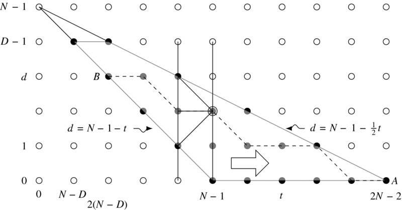
Figure 13.20 The computational space, (t, d), of BBR. Here, D = 5 and N = 6
The side of the trapezoid is defined by the lines,
In the graph, a node (t, d) corresponds to the point in both BBR and BBL:
(Compare this with Equation (13.7).
Instead of designing the circuit from scratch, we can simply modify circuits that have already been designed – in this case, FBR and FBL. One difference between the FB and BB types lies in the direction of the data streams and the number of registers. Another important difference lies in their search spaces. Before designing the circuit, let us first clarify the algorithm. Our objective is to build the circuit, depicted in Figure 13.19, in accordance with the illustration in Figure 13.20.
Algorithm 13.6 (BBR: control) Given Ir = {Ir(0), x, Ir(1), …, Ir(N − 1)} and Il = {Il(0), Il(1), …, Il(N − 1)}, do the following.
- Initialization: for t = 0, 1, …, D − 2, Ili(D − 1) ← Il(t).
- Forward pass: for t = 0, 1, …, N + D − 2, Iri(D − 1) ← Ir(t) and Ili(D − 1) ← Il(t + D − 2).
- Finalization: d(N + D − 2) ← 0.
- Backward pass: for t = N + D − 2, …, 1, 0,
Notice that the time is reduced to N + D − 1 and so is the length of the pointer array. In the initialization state, the left image flows into the array, filling the first D − 1 registers among the 2(D − 1) registers. (Note that each processor has two output registers in the Il ports. Other ports are terminated with a register, for example, in the FB series.) In the forward pass, there is an offset, D − 2, between the left and right image streams. At the end of the left image, the flow continues with D − 2 more values, which may be arbitrary. During the backward pass, the pointers are accumulated and mapped to the pixel in every period.
Because they form a concurrent array, all PE(d), d ∈ [0, D − 1], do identical operations. The major difference with respect to the FB series is the time period and boundary conditions.
Algorithm 13.7 (BBR: processing element) For a processor PE(d), do the following.
- Initialization: for t = 0, 1, …, D − 2, Iro ← Iri, B ← Ili, and Ilo ← B.
- Forward pass: for t = 0, 1, …, N + D − 2, do the following.
- Iro ← Iri, B ← Ili, Ilo ← B, φuo, φdo ← φ.
- If d < D − t − 1 or d > (N + D − 2 − t)/2, η ← 0 and φ ← ∞. else if d = D − t − 1, η(0) ← 0, φ ← |Iri − Ili|, else
- Finalization: a ← I(d = 0).
- Backward pass: for t = N + D − 1, …, 1, 0,
Note how one buffer, B, is introduced for delay in the left image stream. The algorithms are basic frameworks and so have many details missing; these details are explained in the code section.
For BBL, Ir and Il, are reversed and switched for their ports in the controller. However, the systolic array is exactly the same.
13.17 BBR and BBL Overall Scheme
Some parts of the code are exactly the same as that of the FB system – specifically, header (Listing 13.1), buffer (Listing 13.4), reading and writing (Listing 13.5), and preprocessing (Listing 13.6) – and so only the remaining parts (i.e. the parts that are different), namely, initialization, forward pass, finalization, and backtracking, are explained in the following.
Algorithm 13.6 is realized by the code, processor.v. The overall framework of the code is:
Listing 13.13 The framework: processor.v
Conceptually, the code realizes the circuit in Figure 13.19. The code consists of four parts: procedural block, instantiation, data input, and data output. The procedural block realizes the state diagram in Figure 13.14(a). Instantiation is done to build the systolic array, SYSTOLIC, linking individual processing elements with net arrays. Through the links, the streams of image (Il and Ir), cost (φ), and activation bits (a) flow upwards and downwards, so that an element can receive the necessary data from both neighbors and send the processed data to both neighbors. Note also that the processors located on the top and bottom of the array miss one of the two neighbors and thus must be terminated properly. The terminal values are φ = ∞ and a = 0. In this manner, all the elements execute the same neighborhood operations without worrying about their positions. This control unit also plays the role of driver, supplying the array with two image streams, in the same direction. In BBR, the first port, with one buffer register, is for the right image and the second port, with two buffer registers, is for the left image. In BBL, the roles of the two images are changed. Finally, the output is the pointers from the array. Of the D elements, only one emits a valid pointer, a two-bit binary, while the others are either tri-states or zero. To detect the valid pointer, we can combine all the output lines via wired-OR logic (see the problems at the end of this chapter).
The code for the processing element, systolic.v, is used to realize Algorithm 13.7. This code is instantiated by the control unit to form an array of D elements. Each element executes the same operations, depending only on the time and processor ID. The ID is assigned at the time of instantiation and is kept by the synchronized clock. Thus, no handshake is needed, sparing unnecessary communication overhead. The system behaves like an engine, in which all the operations are predetermined by the clock and processor identification.

Listing 13.14 The framework: systolic.v
The code comprises four parts: procedural block, data output, and cost computation. The procedural block is the companion to that of the control unit. The data output drives the ports to send the costs, activation bits, and the pointer. In the internal operation, local cost is needed in order to update parent costs. Therefore, the inputs are compared with appropriate distance measures. The template shows a basic example, in which all the six channels are compared for absolute distance measure. The basic scheme is to assign the first three channels to the RGB images and the remaining channels to the feature maps. However, the number of channels is variable and any assignment to deal with various types of images is possible.
13.18 BBR and BBL Initialization
This part of the code realizes the initiation in Algorithms 13.6 and 13.7. In these algorithms, the two image streams flow into the array in a head-first manner. The purpose is to align the two image streams before the main operation begins. The left image always leads the right image by D − 1 clocks; thus, in this stage the first D − 2 registers are filled with the left image first. Then, at D − 1 clock tick, the two streams first meet at PE(D − 1). In BBL, the streams flow in a tail-first manner and the right image stream fills the array before the left image stream.
The control unit must build two streams of feature vectors from the image buffers, and possibly with the disparity buffer, and supply them on the top of the array.
Listing 13.15 Initialization: processor.v
Unlike FBR and FBL, the streams are not interleaved and the coding is straightforward. The code is switched from BBR and BBL by the Verilog compiler directive.
On the array side, the system is originally in an idle state, waiting for the semaphore from the control unit. As soon as this bit enters, the state changes to the initialization process. There exists one clock tick, and thus the signal is sent just before entering this initiation state in the control side.

Listing 13.16 Initialization: systolic.v
At this instance, the control and array are in perfect synchrony. Each processor passes the downstream for the determined times, i.e. D − 2. There is a difference in FB and BB circuits in the amount of delays. That is, there is a new buffer in the side of the left image stream and thus the input stream must pass two registers before coming out of an element.
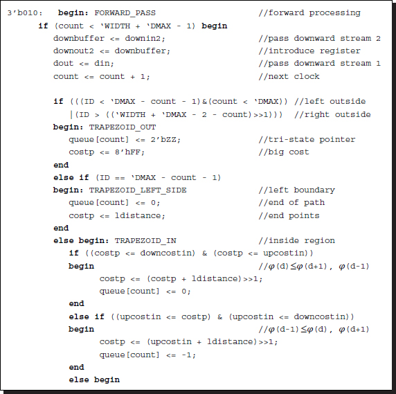
13.19 BBR and BBL Forward Pass
Compared to the FB algorithm, the forward pass in Algorithms 13.6 and 13.7 has a lot of differences, especially in the systolic array.
On the control unit side, the code is relatively simple because the image streams flow in their original ordering, without any interpolation involved. The period of this state is N + D − 2, greatly depending on the disparity level. Compared with the period, 2N − 2, in the FB algorithm, we expect that this algorithm is potentially very fast.
Listing 13.17 Forward pass: processor.v
The control unit constructs two image streams by concatenating one or more channels from the image buffers. The two streams flow in either a head-first (right reference) or a tail-first (left reference) manner. Between the two streams, there is a D − 1 delay. The stream must be a smooth continuation from that of initialization.
On the systolic array side, the goal is to determine the pointers and update the costs. This is the most delicate part of the BBR circuit.
Listing 13.18 Forward pass: systolic.v
As in the FB circuit, the operation depends on where the element is located in (t, d) space, which is characterized by the trapezoid. In the BB circuit, the shape of the trapezoid is somewhat complicated. Because the left side is slanted, one more region appears on the left side of the search space. The first case is when the position is located completely outside of the trapezoid. In this case, the cost is assigned a large number and the pointer is assigned tri-state, because it may not affect the bus when connected with other elements. The second case is when the position is on the left side of the trapezoid, which is the end position in the backtracking. Therefore, the cost and pointer are assigned with local cost and zero pointer, respectively. Inside the trapezoid, the normal forward operations must be performed. The basic operation is to compare the neighbor costs in deciding on the parent. The pointer is an incremental disparity relative to the current node. This operation is the same for the terminal elements in the bottom or top of the array because those processors are terminated with very large costs, which prevent the possible shortest path from advancing in those positions.
As shown in Listing 13.14, the local cost is computed with the image inputs by the combinational circuit. This part, in particular, must be changed in more advanced schemes.
13.20 BBR and BBL Backward Pass
In Algorithms 13.6 and 13.7, the finalization is the computation stage that follows the forward pass and appears before the backward pass. The purpose of this stage is to choose a starting point for the backward pass. The starting point must be a node whose cost is minimal among the nodes in the final column. In BBR and BBL, this point is fixed to the point of the trapezoid, that is PE(0), making this stage almost trivial.
Unlike FB circuits, this part is somewhat complicated because of the introduction of a new region in the search space. The region, outside of the left side, must be passed, with no effect on the accumulation and pixel mapping. The more important operation is to compensate the missing pixels when η = −1. The circuits are characterized with the three parent candidates, (t − 1, d), (t − 1, d + 1), and (t − 1, d − 1). Of the three candidate parents, (t − 1, d + 1) and (t − 1, d) map to the same pixel, xr, meaning step changes in disparity. The point (t − 1, d − 1), however, maps to xr − 2, meaning that xr − 1 is undetermined. Therefore, we have to fill this position, with the disparity at either of the two ends.
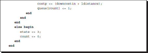
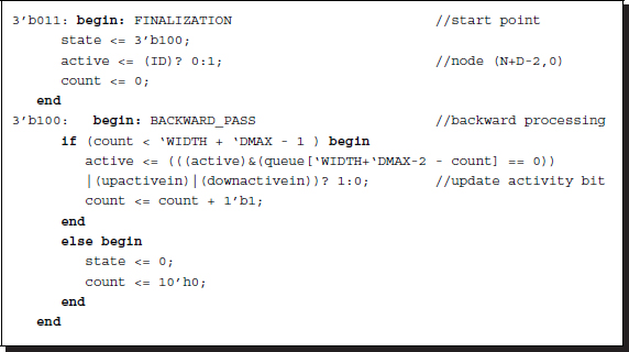
Listing 13.19 Backward pass: processor.v
The disparity value is computed by the combinational circuit in Listing 13.13. The concept is as follows. Each element issues a disparity output to the common bus. Of the D elements, only one element outputs the disparity; all others output tri-state. Therefore, the feasible output can be detected by wired-OR logic. In addition, the computation region must be restricted, because the path ends early at the left side of the trapezoid; thus, the disparity sequence may be shorter than N + D − 2.
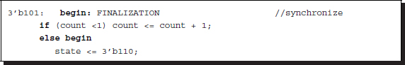
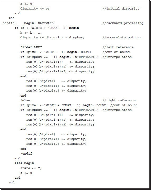
In the systolic element, the backward pass reads as follows:
Listing 13.20 Backward pass: systolic.v
The active bits are the major mechanism to trace back the shortest path. The disparity output is computed by the combinational circuit in Listing 13.14. A somewhat complicated situation occurs when the computation crosses the region left of the trapezoid: in order not to affect the accumulation operation, the pointer is set to zero.
A review of the codes shows that this circuit is simpler than FB in data streaming but complicated in its management of boundary conditions. Interleaving is not involved in the filling of the empty pixels, but interpolation is. We can expect the disparity result to be jumpy on the right side and smooth on the left side in the BBR circuit. The reverse holds for the BBL circuit.
13.21 BBR and BBL Simulation
We used sample images – a pair of 225 × 188 images-to test BBR and BBL. Figure 13.21 depicts the simulation results. Three lines are used in computing local distance in four-neighborhood. The images in the second row are the respective disparity maps for left reference and right reference. Notably, the left side is poor in the left reference and vice versa for the right reference. The disparity maps for the center reference are placed in the third row. The disparity map is mapped to the left image plane and the right image plane.

Figure 13.21 Disparity maps: four-neighborhood operations (D = 32)
By comparing the two sets of simulations – FB and BB, a difference can easily be seen. The FB circuits provide better performance. One of the reasons for this is that in BB circuits one of the three parent nodes is abnormal. Unlike FB circuits, in which all three candidate nodes denote three different pixels, in a BB circuit one of the parent nodes maps to the same pixel. In addition, the other parent candidate maps to the pixel that is two units away from the current pixel. Therefore, the pixel that is skipped must be interpolated one way or another. The template simply copies the previous node to fill in for the node that has been skipped, which may raise problems around boundaries.
From a performance standpoint, the FB series appears to be better than the BB series circuits. Conversely, from a computational standpoint, the opposite holds. The FB series is somewhat complicated because of the need for leading delays in the image streams and the use of interleaving. The BB series does not need such complications; the left boundary of the trapezoid is instead somewhat complicated, resulting in the array element needing more logic. In the BB series, the computation range is significantly shorter, specifically, N + D, than 2N − 1 in the FB series.
The eight fundamental circuits are defined in Figure 13.6. Of these eight circuits, we have so far designed only four: FBR, FBL, BBR, and BBL. The remaining circuits, BFR, BFL, FFR, and FFL, can however be derived from FBR, FBL, BBR, and BBL, respectively, by inverting either their data directions or their data streams. The duality occurs due to their coordinates systems, stream directions, and data directions.
The DP algorithm for stereo matching has been realized in two directions: a single processor (specifically, a DP machine) and an array (specifically, a systolic machine), in Chapter 12 and in this chapter, respectively. As all the circuits are now available, we can compare the two systems. From a computational standpoint, the array implementation is very fast: O(N2D) vs. O(N). One of the reasons is the fact that the D nodes are executed serially in single processors while they are processed concurrently in array processors. It is natural that the need for space is opposite to the need for speed. The other reason is that there is a full range of parent candidates in the single processor while it is limited to neighborhoods in the array processor. The smaller neighborhood contributes a speed factor of N to the array processor. Thus, from a performance standpoint, the single processor is much better than the array processor. The main reason is of course the wider neighborhood range.
In any case, the DP algorithm is based on line processing, which is naturally faster than the others, but is destined to be poorer than frame processing. The results are always horizontal noise (or vertical instability), because the lines are processed independently. To compensate for this weakness, we can use various methods. One such method is to combine the results from the right and left references. This requires some kind of occlusion detection and a filling of the gaps with suitable disparity. Another method is preprocessing for vertical smoothing, because the line-based method is poor in the vertical variation. To remedy the vertical independence, we may rely on segmentation such as soft matting. When the segmented result is used as the input features, the resulting disparity map is more likely to be stable in vertical variation. The final attempt might be the fusion of other vision modules or the expanded DP, which may help the stereo matching.
Problems
- 13.1 [Systolic transform] In the text, the possibility of many more equivalent circuits was mentioned. Explain this possibility.
- 13.2 [Systolic transform] In Figure 13.2, the array size is D = 3. For a general D, how many ways are there to route the broadcast paths?
- 13.3 [Systolic transform] In Figure 13.2, the routing is chosen in such a way that the right image enters PE(2). Derive a new circuit in which the right image enters PE(1). Discuss the property of the new circuit in terms of FB and BB type circuits.
- 13.4 [Systolic transform] Repeat the previous problem for the circuit in Figure 13.4.
- 13.5 [Systolic transform] In Figure 13.2, the edges are multiplied by two for the number of registers, and the resulting system becomes an interleaved circuit, called 2-slow. This operation must affect both the number of registers and the input streams. Derive an equivalent circuit that is 3-slow. Check the correctness of the circuit by counting the number of delays from each node.
- 13.6 [Systolic transform] It is possible to create another circuit from the above circuit by distributing the registers differently. Derive the equivalent circuit that has the registers distributed differently.
- 13.7 [Systolic transform] By analyzing the previous two examples, draw a general principle for k-slow circuits.
- 13.8 [Systolic algorithm] In FBR, what are the coordinates of the parent nodes? What kind of performance can be expected from such a parent formation?
- 13.9 [Systolic algorithm] Repeat the same discussion as above for BBR (Figure 13.6(e)).
- 13.10 [Overall scheme] In Listings 13.2 and 13.13, the output of the D elements are gathered by wired-OR.

If the elements emit 2'b00 instead of 2'bZZ, how must this combinational circuit be changed?
- 13.11 [Overall scheme] Discuss the new ideas for improving the systolic arrays.
References
- Jeong H 1984 Modeling and transformation of systolic network Master's thesis Massachusetts Institute of Technology.
- Jeong H and Oh Y 2000 Trellis-based parallel stereo matching Proceedings of the IEEE International Conference on Acoustics, Speech, and Signal Processing, Istanbul, Turkey.
- Jeong H and Yuns O 2000 Fast stereo matching using constraints in discrete space. IEICE Transactions on Information and Systems 83(7), 1592–1600.
- Jeong H, Oh Y, Park J, Koo B, and Lee SW 2002 Vision-based adaptive and recursive tracking of unpaved roads. Pattern Recognition Letters 23(1), 73–82.
- Kung H and Leiserson C 1980 Algorithms for VLSI processor arrays In Introduction to VLSI Systems (ed. Mead C and Conway L) Addison-Wesley Reading, MA pp. 271–291.
- Leiserson C and Saxe J 1991 Retiming synchronous circuitry. Algorithmica 6(1), 5–35.