Chapter 19. Data Compression

Data reduction or compression techniques are important because universal laws put a premium on information. You couldn’t read all the books in the world, neither could you store them. You might make a start on reading every book by making it a team effort. In other words, you might tackle the problem with more than one brain and one pair of eyes. In communication theory terms, this approach is known as increasing the channel capacity by broadening the bandwidth. But you wouldn’t have an infinite number of people at your disposal unless you had an infinite amount of money to pay them! Likewise no one has an infinite channel capacity or an infinite bandwidth at their disposal. The similar argument applies to storage. Stated axiomatically: information, in all its forms, is using up valuable resources, so the more efficiently we can send it and store it the better. That’s where compression comes in.

If I say to you, “Wow, I had a bad night, the baby cried from three ‘til six!” You understand perfectly what I mean because you know what a baby crying sounds like. I might alternatively have said, “Wow, I had a bad night, the baby did this; wah, bwah, bwah, wah …” and continue doing it for 3 h. Try it. You’ll find you lose a lot of friends because nobody needs to have it demonstrated. Most of the 3-h impersonation is superfluous. The second message is said to have a high level of redundancy in the terms of communication theory. The trick performed by any compression system is sorting out the necessary information content—sometimes called the entropy—from the redundancy. (If, like me, you find it difficult to comprehend the use of entropy in this context consider this: entropy refers here to a lack of pattern; to disorder. Everything in a signal that has a pattern is, by definition, predictable and therefore redundant. Only those parts of the signal that possess no pattern are unpredictable and therefore represent necessary information.)

All compression techniques may be divided between lossless systems and lossy systems. Lossless compression makes use of efficiency gains in the manner in which data are coded. All that is required to recover original data exactly is a decoder that implements the reverse process performed by the coder. Such a system does not confuse entropy for redundancy and hence dispense with important information. However, neither does the lossless coder perfectly divide entropy from redundancy. A good deal of redundancy remains and a lossless system is therefore only capable of relatively small compression gains. Lossy compression techniques attempt a more complete distinction between entropy and redundancy by relying on knowledge of the predictive powers of the human perceptual systems. This explains why these systems are referred to as implementing perceptual coding techniques. Unfortunately, not only are these systems inherently more complicated, they are also more likely to get things wrong and produce artifacts.

19.1. Lossless Compression

Consider the following contiguous stream of luminance bytes taken from a bit-map graphic:

• 00101011
• 00101011
• 00101011
• 00101011
• 00101011
• 00101011
• 00101100
• 00101100
• 00101100
• 00101100
• 00101100

There must be a more efficient way of coding this! “Six lots of 00101011 followed by five lots of 00101100” springs to mind. Like this:

• 00000110
• 00101011
• 00000101
• 00101100

This is the essence of a compression technique known as run-length encoding (RLE). RLE works really well but it has a problem. If a data file is composed of data that are predominantly nonrepetitive, RLE actually makes the file bigger! So RLE must be made adaptive so that it is only applied to strings of similar data (where redundancy is high); when the coder detects continuously changing data (where entropy is high), it simply reverts back to sending the bytes in an uncompressed form. Evidently it also has to insert a small information overhead to instruct the decoder when it is (and isn’t) applying the compression algorithm.

Another lossless compression technique is known as Huffman coding and is suitable for use with signals in which sample values appear with a known statistical frequency. The analogy with Morse code is frequently drawn, in which letters that appear frequently are allocated simple patterns and letters that appear rarely are allocated more complex patterns. A similar technique, known by the splendid name of the Lempel-Ziv-Welch (LZW) algorithm, is based on the coding of repeated data chains or patterns. A bit like Huffman’s coding, LZW sets up a table of common patterns and codes specific instances of patterns in terms of “pointers,” which refer to much longer sequences in the table. The algorithm doesn’t use a predefined set of patterns but instead builds up a table of patterns that it “sees” from incoming data. LZW is a very effective technique—even better than RLE. However, for the really high compression ratios, made necessary by the transmission and storage of high-quality audio down low bandwidth links, different approaches are required, based on an understanding of human perception processes.

In principle, the engineering problem presented by low-data rates, and therefore in reduced digital resolution, is no different to the age-old analogue problems of reduced dynamic range. In analogue systems, noise reduction systems (either complementary, i.e., involving encoding and complementary decoding such as Dolby B and dbx1, or single ended) have been used for many years to enhance the dynamic range of inherently noisy transmission systems such as analogue tape. All of these analogue systems rely on a method called “compansion,” a word derived from the contraction of compression and expansion. The dynamic range is deliberately reduced (compressed) in the recording stage processing and recovered (expanded) in the playback electronics. In some systems this compansion acts over the whole frequency range (dbx is one such type). Others work over a selected frequency range (Dolby A, B, C, and SR). We shall see that the principle of compansion applies in just the same way to digital systems of data reduction. Furthermore, the distinction made between systems that act across the whole audio frequency spectrum and those that act selectively on ranges of frequencies (subbands) is true too of digital implementations. However, digital systems have carried the principle of subband working to a sophistication undreamed of in analogue implementations.

19.2. Intermediate Compression Systems

Consider the 8-bit digital values: 00001101, 00011010, 00110100, 0110100, and 11010000. (Eight bit examples are used because the process is easier to follow but the following principles apply in just the same way to digital audio samples of 16 bits or, indeed, any word length.) We might just as correctly write these values thus:

00001101	=	1101	*	1
00011010	=	1101	*	10
00110100	=	1101	*	100
01101000	=	1101	*	1000
11010000	=	1101	*	10000

If you think of the multipliers 1, 10, 100, and so on as powers of two then it’s pretty easy to appreciate that the representation given earlier is a logarithmic description (to the log of base two) with a 4-bit mantissa and a 3-bit exponent. So already we’ve saved 1 bit in 8 (a 20% data reduction). We’ve paid a price of course because we’ve sacrificed accuracy in the larger values by truncating the mantissas to 4 bits. However, this is possible in any case with audio because of the principle of masking, which underlies the operation of all noise reduction systems. Put at its simplest, masking is the reason we strain to listen to a conversation on a busy street and why we cannot hear the clock ticking when the television set is on: loud sounds mask quiet ones. So the logarithmic representation makes sense because resolution is maintained at low levels but sacrificed at high levels where the program signal will mask the resulting, relatively small, quantization errors.

19.2.1. NICAM

Further reductions may be made because real audio signals do not change instantaneously from very large to very small values, so the exponent value may be sent less often than the mantissas. This is the principle behind the stereo television technique of NICAM, which stands for near instantaneous companded audio multiplex. In NICAM 782, 14-bit samples are converted to 10-bit mantissas in blocks of 32 samples with a common 3-bit exponent. This is an excellent and straightforward technique but it is only possible to secure relatively small reductions in data throughput of around 30%.

19.3. Psychoacoustic Masking Systems

Wideband compansion systems view the phenomenon of masking very simply and rely on the fact that program material will mask system noise. But, actually masking is a more complex phenomenon. Essentially it operates in frequency bands and is related to the way in which the human ear performs a mechanical Fourier analysis of the incoming acoustic signal. It turns out that a loud sound only masks a quieter one when the louder sound is lower in frequency than the quieter, and only then, when both signals are relatively close in frequency. It is due to this effect that all wideband compansion systems can only achieve relatively small gains. The more data we want to discard the more subtle must our data reduction algorithm be in its appreciation of the human masking phenomena. These compression systems are termed psychoacoustic systems and, as you will see, some systems are very subtle indeed.

19.4. MPEG Layer 1 Compression (PASC)

It’s not stretching the truth too much to say that the failed Philips’ digital compact cassette (DCC) system was the first nonprofessional digital audio tape format. As we have seen, other digital audio developments had ridden on the back of video technology. The CD rose from the ashes of Philips Laserdisc, and DAT machines use the spinning-head tape recording technique originally developed for B and C-Format 1-inch video machines, later exploited in U-Matic and domestic videotape recorders. To their credit then, that, in developing the DCC, Philips chose not to follow so many other manufacturers down the route of modified video technology. Inside a DCC machine, there’s no head wrap, no spinning head, and few moving precision parts. Until DCC, it had taken a medium suitable for recording the complex signal of a color television picture to store the sheer amount of information needed for a high-quality digital audio signal. Philips’ remarkable technological breakthrough in squeezing two high-quality, stereo digital audio channels into a final data rate of 384 kBaud was accomplished by, quite simply, dispensing with the majority (75%) of the digital audio data! Philips named their technique of bit-rate reduction or data-rate compression precision adaptive sub-band coding (PASC). PASC was adopted as the original audio compression scheme for MPEG video/audio coding (layer 1).

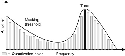
In MPEG layer 1 or PASC audio coding, the whole audio band is divided up into 32 frequency subbands by means of a digital wave filter. At first sight, it might seem that this process will increase the amount of data to be handled tremendously—or by 32 times anyway! This, in fact, is not the case because the output of the filter bank, for any one frequency band, is at 1/32nd of the original sampling rate. If this sounds counterintuitive, take a look at the Fourier transform and note that a very similar process is performed here. Observe that when a periodic waveform is sampled n times and transformed, the result is composed of n frequency components. Imagine computing the transform over a 32- sample period: 32 separate calculations will yield 32 values. In other words, the data rate is the same in the frequency domain as it is in the time domain. Actually, considering that both describe exactly the same thing with exactly the same degree of accuracy, this shouldn’t be surprising. Once split into subbands, sample values are expressed in terms of a mantissa and exponent exactly as explained earlier. Audio is then grouped into discrete time periods, and the maximum magnitude in each block is used to establish the masking “profile” at any one moment and thus predict the mantissa accuracy to which the samples in that subband can be reduced, without their quantization errors becoming perceivable (see Figure 19.1).

Figure 19.1. Subband quantization and how it relates to the masking profile.

Despite the commercial failure of DCC, the techniques employed in PASC are indicative of techniques now widely used in the digital audio industry. All bit-rate reduction coders have the same basic architecture, pioneered in PASC: however, details differ. All systems accept PCM dual channel, digital audio (in the form of one or more AES pairs) is windowed over small time periods and transformed into the frequency domain by means of subband filters or via a transform filter bank. Masking effects are then computed based on a psychoacoustic model of the ear. Note that blocks of sample values are used in the calculation of masking. Because of the temporal, as well as frequency dependent, effects of masking, it’s not necessary to compute masking on a sample-by-sample basis. However, the time period over which the transform is performed and the masking effects computed are often made variable so that quasi-steady-state signals are treated rather differently to transients. If coders do not include this modification, masking can be predicted incorrectly, resulting in a rush of quantization noise just prior to a transient sound. Subjectively this sounds like a type of pre-echo. Once the effects of masking are known, the bit allocation routine apportions the available bit rate so that quantization noise is acceptably low in each frequency region. Finally, ancillary data are sometimes added and the bit stream is formatted and encoded.

19.4.1. Intensity Stereo Coding

Because of the ear’s insensitivity to phase response above about 2 kHz, further coding gains can be achieved by sending by coding the derived signals (L+R) and (L−R) rather than the original left and right channel signals. Once these signals have been transformed into the frequency domain, only spectral amplitude data are coded in the HF region; the phase component is simply ignored.

19.4.2. The Discrete Cosine Transform

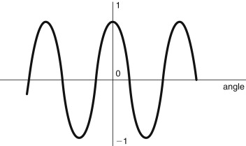
The encoded data’s similarity to a Fourier transform representation has already been noted. Indeed, in a process developed for a very similar application, Sony’s compression scheme for MiniDisc actually uses a frequency domain representation utilizing a variation of the discrete fourier transform (DFT) method known as the discrete cosine transform (DCT). The DCT takes advantage of a distinguishing feature of the cosine function, which is illustrated in Figure 19.2, that the cosine curve is symmetrical about the time origin. In fact, it’s true to say that any waveform that is symmetrical about an arbitrary “origin” is made up of solely cosine functions. This is difficult to believe, but consider adding other cosine functions to the curve illustrated in Figure 19.2. It doesn’t matter what size or what period waves you add, the curve will always be symmetrical about the origin. Now, it would obviously be a great help, when we come to perform a Fourier transform, if we knew the function to be transformed was only made up of cosines because that would cut down the maths by half. This is exactly what is done in the DCT. A sequence of samples from the incoming waveform is stored and reflected about an origin. Then one-half of the Fourier transform performed. When the waveform is inverse transformed, the front half of the waveform is simple ignored, revealing the original structure.

Figure 19.2. Cosine function.

19.5. MPEG Layer 2 Audio Coding (MUSICAM)

The MPEG layer 2 algorithm is the preferred algorithm for European DTV and includes a number of simple enhancements of layer 1 (or PASC). Layer 2 was originally adopted as the transmission coding standard for the European digital radio project (Digital Audio Broadcasting or DAB) where it was termed MUSICAM. The full range of bit rates for each layer is supported, as are all three sampling frequencies, 32, 44.1, and 48 kHz. Note that MPEG decoders are always backward compatible, that is, a layer 2 decoder can decode layer 1 or layer 2 bit streams; however, a layer 2 decoder cannot decode a layer 3-encoded stream.

MPEG layer 2 coding improves compression performance by coding data in larger groups. The layer 2 encoder forms frames of 3 by 12 by 32=1152 samples per audio channel. Whereas layer 1 codes data in single groups of 12 samples for each subband, layer 2 codes data in three groups of 12 samples for each subband. The encoder encodes with a unique scale factor for each group of 12 samples only if necessary to avoid audible distortion. The encoder shares scale factor values between two or all three groups when the values of the scale factors are sufficiently close or when the encoder anticipates that temporal noise masking will hide the consequent distortion. The layer 2 algorithm also improves performance over layer 1 by representing the bit allocation, the scale factor values, and the quantized samples with a more efficient code. Layer 2 coding also added 5.1 multichannel capability. This was done in a scaleable way so as to be compatible with layer 1 audio.

MPEG layers 1 and 2 contain a number of engineering compromises. The most severe concerns the 32 constant-width subbands which do not reflect accurately the equivalent filters in the human hearing system (the critical bands). Specifically, the bandwidth is too wide for the lower frequencies so the number of quantizer bits cannot be specifically tuned for the noise sensitivity within each critical band. Furthermore, the filters have insufficient Q so that signal at a single frequency can affect two adjacent filter bank outputs. Another limitation concerns the time frequency–time domain transformations achieved with the wave filter. These are not transparent so, even without quantization, the inverse transformation would not perfectly recover the original input signal.

19.6. MPEG Layer 3

The layer 3 algorithm is a much more refined approach. Layer 3 is finding its application on the Internet where the ability to compress audio files by a large factor is important in download times. In layer 3, time to frequency mapping is performed by a hybrid filter bank composed of the 512-tap polyphase quadrature mirror filter (used in layers 1 and 2) followed by an 18-point modified cosine transform filter. This produces a signal in 576 bands (or 192 bands during a transient). Masking is computed using a 1024-point FFT: once again more refined than the 512-point FFT used in layers 1 and 2. This extra complexity accounts for the increased coding gains achieved with layer 3, but increases the time delay of the coding process considerably. Of course, this is of no account at all when the result is an encoded .mp3 file.

19.6.1. Dolby AC-3

The analogy between data compression systems and noise reduction has already been drawn. It should therefore come as no surprise that one of the leading players in audio data compression should be Dolby, with that company’s unrivaled track record in noise reduction systems for analogue magnetic tape. Dolby AC-3 is the adopted coding standard for terrestrial digital television in the United States; however, it was actually implemented for the cinema first, where it was called Dolby Digital. It was developed to provide multichannel digital sound with 35-mm prints. In order to retain an analogue track so that these prints could play in any cinema, it was decided to place the new digital optical track between the sprocket holes, as illustrated in Figure 19.3. The physical space limitation (rather than crude bandwidth) was thereby a key factor in defining its maximum practical bit rate. Dolby Labs did a great deal of work to find a channel format that would best satisfy the requirements of theatrical film presentation. They discovered that five discrete channels—left (L), right (R), center (C), left surround (LS), and right surround (RS)—set the right balance between realism and profligacy! To this they added a limited (1/10th) bandwidth subwoofer channel; the resulting system being termed 5.1 channels. Dolby Digital provided Dolby Labs a unique springboard for consumer formats for the new DTV (ATSC) systems.

Figure 19.3. Dolby Digital as originally coded on film stock.

Like MPEG, AC-3 divides the audio spectrum of each channel into narrow frequency bands of different sizes optimized with respect to the frequency selectivity of human hearing. This makes it possible to sharply filter coding noise so that it is forced to stay very close in frequency to the frequency components of the audio signal being coded. By reducing or eliminating coding noise wherever there are no audio signals to mask it, the sound quality of the original signal can be preserved subjectively. In this key respect, a perceptual coding system such as AC-3 is essentially a form of very selective and powerful Dolby-A type noise reduction! Typical final data-rate applications include 384 kb/s for 5.1-channel Dolby Surround Digital consumer formats and 192 kb/s for two-channel audio distribution.

19.6.2. Dolby E

Dolby E is a digital audio compression technology designed for use by TV broadcast and production professionals which allows an AES/EBU audio pair to carry up to eight channels of digital audio. Because the coded audio frame is arranged to be synchronous with the video frame, encoded audio can be edited without mutes or clicks. Dolby E can be recorded on a studio-level digital VTR and switched or edited just like any other AES digital audio signal, as long as some basic precautions are observed. Data must not be altered by any part of the system it passes through. That’s to say, the gain must not be changed, data must not be truncated or dithered, and neither must the sample rate be converted. Dolby E technology is designed to work with most popular international video standards. In its first implementation, Dolby E supported 29.97 fps, 20-bit word size, and 48-kHz audio. Newer versions will support 25 fps, 24 fps, and 16-bit and 24-bit audio.

19.6.3. DTS

DTS, the rival to Dolby Digital in the cinema, uses an entirely different approach to AC-3-coded data on film stock. In DTS, the digital sound (up to 10 channels and a subwoofer channel) are recorded on CDs, which are synchronized to the film by means of a time code. Because of the higher data rate available (CD against optical film track), DTS uses a relatively low 4:1 compression ratio.

19.6.4. MPEG AAC

MPEG-2 advanced audio coding (AAC) was finalized as a standard in 1997 (ISO/IEC 13818–7). AAC constitutes the coding algorithms of the new MPEG-4 standard.

19.7. MPEG-4

MPEG-4 will define a method of describing objects (both visual and audible) and how they are “composited” and interact together to form “scenes.” The scene description part of the MPEG-4 standard describes a format for transmitting the spatiotemporal positioning information that describes how individual audiovisual objects are composed within a scene. A “real world” audio object is defined as an audible semantic entity recorded with one microphone—in case of a mono recording—or with more microphones, at different positions, in case of a multichannel recording. Audio objects can be grouped or mixed together, but objects cannot be split easily into subobjects. Applications for MPEG-4 audio might include “mix minus 1” applications in which an orchestra is recorded minus the concerto instrument, allowing a musician to play along with his or her instrument at home, or where all effects and music tracks in a feature film are “mix minus the dialogue,” allowing very flexible multilingual applications because each language is a separate audio object and can be selected as required in the decoder.

In principle, none of these applications is anything but straightforward; they could be handled by existing digital (or analogue) systems. The problem, once again, is bandwidth. MPEG-4 is designed for very low bit rates and this should suggest that MPEG have designed (or integrated) a number of very powerful audio tools to reduce necessary data throughput. These tools include the MPEG-4 Structured Audio format, which uses low bit-rate algorithmic sound models to code sounds. Furthermore, MPEG-4 includes the functionality to use and control postproduction panning and reverberation effects at the decoder, as well as the use of a SAOL signal-processing language enabling music synthesis and sound effects to be generated, once again, at the terminal rather than prior to transmission.

19.7.1. Structured Audio

We have already seen how MPEG (and Dolby) coding aims to remove perceptual redundancy from an audio signal, as well as removing other simpler representational redundancy by means of efficient bit-coding schemes. Structured audio (SA) compression schemes compress sound by, first, exploiting another type of redundancy in signals—structural redundancy.

Structural redundancy is a natural result of the way sound is created in human situations. The same sounds, or sounds which are very similar, occur over and over again. For example, a performance of a work for solo piano consists of many piano notes. Each time the performer strikes the “middle C” key on the piano, a very similar sound is created by the piano’s mechanism. To a first approximation, we could view the sound as exactly the same upon each strike; to a closer one, we could view it as the same except for the velocity with which the key is struck and so on. In a PCM representation of the piano performance, each note is treated as a completely independent entity; each time the “middle C” is struck, the sound of that note is independently represented in the data sequence. This is even true in a perceptual coding of the sound. The representation has been compressed, but the structural redundancy present in rerepresenting the same note as different events has not been removed.

In structured coding, we assume that each occurrence of a particular note is the same, except for a difference described by an algorithm with a few parameters. In the model-transmission stage we transmit the basic sound (either a sound sample or another algorithm) and the algorithm which describes the differences. Then, for sound transmission, we need only code the note desired, the time of occurrence, and the parameters controlling the differentiating algorithm.

19.7.2. SAOL

SAOL (pronounced “sail”) stands for “Structured Audio Orchestra Language” and falls into the music-synthesis category of “Music V” languages. Its fundamental processing model is based on the interaction of oscillators running at various rates. Note that this approach is different from the idea (used in the multimedia world) of using MIDI information to drive synthesis chips on sound cards. This latter approach has the disadvantage that, depending on IC technology, music will sound different depending on which sound card is realized. Using SAOL (a much “lower-level” language than MIDI) realizations will always sound the same.

At the beginning of an MPEG-4 session involving SA, the server transmits to the client a stream information header, which contains a number of data elements. The most important of these is the orchestra chunk, which contains a tokenized representation of a program written in SAOL. The orchestra chunk consists of the description of a number of instruments. Each instrument is a single parametric signal-processing element that maps a set of parametric controls to a sound. For example, a SAOL instrument might describe a physical model of a plucked string. The model is transmitted through code, which implements it, using the repertoire of delay lines, digital filters, fractional-delay interpolators, and so forth that are the basic building blocks of SAOL.

The bit stream data itself, which follows the header, is made up mainly of time-stamped parametric events. Each event refers to an instrument described in the orchestra chunk in the header and provides the parameters required for that instrument. Other sorts of data may also be conveyed in the bit stream; tempo and pitch changes, for example.

Unfortunately, at the time of writing (and probably for some time beyond!) the techniques required for automatically producing a structured audio bit stream from an arbitrary, prerecorded sound are beyond today’s state of the art, although they are an active research topic. These techniques are often called “automatic source separation” or “automatic transcription.” In the meantime, composers and sound designers will use special content creation tools to directly create SA bit streams. This is not considered to be a fundamental obstacle to the use of MPEG-4 structured audio because these tools are very similar to the ones that contemporary composers and editors use already; all that is required is to make their tools capable of producing MPEG-4 output bit streams. There is an interesting corollary here with MPEG-4 for video. For, while we are not yet capable of integrating and coding real-world images and sounds, there are immediate applications for directly synthesized programs. MPEG-4 audio also foresees the use of text-to-speech conversion systems.

19.7.3. Audio Scenes

Just as video scenes are made from visual objects, audio scenes may be usefully described as the spatiotemporal combination of audio objects. An “audio object” is a single audio stream coded using one of the MPEG-4 coding tools, such as structured audio. Audio objects are related to each other by mixing, effects processing, switching, and delaying them, and may be panned to a particular three-dimensional location. The effects processing is described abstractly in terms of a signal-processing language—the same language used for SA.

19.8. Digital Audio Production

We’ve already looked at the technical advantages of digital signal processing and recording over its older analogue counterpart. We now come to consider the operational impact of this technology, where it has brought with it a raft of new tools and some new problems.