Chapter 27. Recording Consoles

27.1. Introduction

This chapter is about recording consoles, the very heart of a recording studio. Like our own heart, whose action is felt everywhere in our own bodies, consideration of a recording console involves wide-ranging considerations of other elements within the studio system. These, too, are covered in this chapter.

In pop and rock music, as well as in most jazz recordings, each instrument is almost always recorded onto one track of multitrack tape and the result of the “mix” of all the instruments combined together electrically inside the audio mixer and recorded onto a two-track (stereo) master tape for production and archiving purposes. Similarly, in the case of sound reinforcement for rock and pop music and jazz concerts, each individual musical contributor is miked separately and the ensemble sound mixed electrically. It is the job of the recording or balance engineer to control this process. This involves many aesthetic judgements in the process of recording the individual tracks (tracking) and mixing down the final result. However, relatively few parameters exist under her/his control. Over and above the office of correctly setting the input gain control so as to ensure best signal to noise ratio and control of channel equalization, her/his main duty is to judge and adjust each channel gain fader and therefore each contributor’s level within the mix. A further duty, when performing a stereo mix, is the construction of a stereo picture or image by controlling the relative contribution each input channel makes to the two, stereo mix amplifiers. In cases of both multitrack mixing and multimicrophone mixing, the apparent position of each instrumentalist within the stereo picture (image) is controlled by a special stereophonic panoramic potentiometer, or pan pot for short.

27.2. Standard Levels and Level Meters

Suppose I asked you to put together a device comprising component parts I had previously organized from different sources. And suppose I had paid very little attention to whether each of the component parts would fit together (perhaps one part might be imperial and another metric). You would become frustrated pretty quickly because the task would be impossible. So it would be too for the audio mixer, if the signals it received were not, to some degree at least, standardized. The rationale behind these standards and the tools used in achieving this degree of standardization are the subjects of the first few sections of this chapter.

The adoption of standardized studio levels (and of their associated lineup tones) ensures the interconnectability of different equipment from different manufacturers and ensures that tapes made in one studio are suitable for replay and/or rework in another. Unfortunately, these “standards” have evolved over many years and some organizations have made different decisions, which, in turn, have reflected upon their choice of operating level. National and industrial frontiers exist too, so that the subject of maximum and alignment signal levels is fraught with complication.

Fundamentally, only two absolute levels exist in any electronic system, maximum level, and noise floor. These are both illustrated in Figure 27.1. Any signal that is lower than the noise floor will disappear as it is swamped by noise and signal, which is larger than maximum level will be distorted. All well-recorded signals have to sit comfortably between the “devil” of distortion and the “deep blue sea” of noise. Actually, that’s the fundamental job of any recording engineer!

Figure 27.1. System dynamic range.

In principle, maximum level would make a good line-up level. Unfortunately, it would also reproduce over loudspeakers as a very loud noise indeed and would therefore, likely as not, “fray the nerves” of those people working day after day in recording studios! Instead a lower level is used for line-up, which actually has no physical justification at all. Instead it is cleverly designed to relate maximum signal level to the perceptual mechanism of human hearing and to human sight as we shall see. Why sight? Because it really isn’t practical to monitor the loudness of an audio signal by sound alone. Apart from anything else, human beings are very bad at making this type of subjective judgement. Instead, from the very earliest days of sound engineering, visual indicators have been used to indicate audio level, thereby relieving the operator from making subjective auditory decisions. There exist two important and distinct reasons to monitor audio level.

The first is to optimize the drive, the gain or sensitivity of a particular audio circuit, so that the signal passing through it is at a level whereby it enjoys the full dynamic range available from the circuit. If a signal travels through a circuit at too low a level, it unnecessarily picks up noise in the process. If it is too high, it may be distorted or “clipped” as the stage is unable to provide the necessary voltage swing, as shown in Figure 27.1.

The second role for audio metering exists in, for instance, a radio or television continuity studio where various audio sources are brought together for mixing and switching. Listeners are justifiably entitled to expect a reasonably consistent level when listening to a radio (or television) station and do not expect one program to be unbearably loud (or soft) in relation to the last. In this case, audio metering is used to judge the apparent loudness of a signal and thereby make the appropriate judgements as to whether the next contribution should be reduced (or increased) in level compared with the present signal.

The two operational requirements described earlier demand different criteria of the meter itself. This pressure has led to the evolution of two types of signal monitoring meter, the volume unit (VU) meter, and the peak program meter (PPM).

27.2.1. The VU Meter

A standard VU meter is illustrated in Figure 27.2(a). The VU is a unit intended to express the level of a complex wave in terms of decibels above or below a reference volume, it implies a complex wave—a program waveform with high peaks. A 0 VU reference level therefore refers to a complex-wave power reading on a standard VU meter. A circuit for driving a moving coil VU meter is given in Figure 27.2(b). Note that the rectifiers and meter are fed from the collector of TR^a, which is a current source in parallel with Re. Because Re is a high value in comparison with the emitter load of TR^a the voltage gain during the part of the input cycle when the rectifier diodes are not in conduction is very large. This alleviates most of the problem of the Si diodes’ offset voltage. From the circuit it is clear that a VU meter is an indicator of the average power of a waveform; it therefore accurately represents the apparent loudness of a signal because the ear too mathematically integrates audio waveforms with respect to time. However, because of this, the VU is not a peak-reading instrument. A failure to appreciate this, and on a practical level this means allowing the meter needle to swing into the red section on transients, means that the mixer is operating with inadequate system headroom. This characteristic has led the VU to be regarded with suspicion in some organizations.

Figure 27.2(a). VU meter.

Figure 27.2(b). VU meter circuit.

To some extent, this is unjustified because the VU may be used to monitor peak levels, provided the action of the device is properly understood. The usual convention is to assume that the peaks of the complex wave will be 10 to 14 dB higher than the peak value of a sine wave adjusted to give the same reference reading on the VU meter. In other words, if a music or speech signal is adjusted to give a reading of 0 VU on a VU meter, the system must have at least 14 dB headroom—over the level of a sine wave adjusted to give the same reading—if the system is not to clip the program audio signal. In operation, the meter needles should swing only very occasionally above the 0 VU reference level on complex program.

27.2.2. The PPM Meter

Whereas the VU meter reflects the perceptual mechanism of the human hearing system, and thereby indicates the loudness of a signal, the PPM is designed to indicate the value of peaks of an audio waveform. It has its own powerful champions, notably the BBC and other European broadcasting institutions. The PPM is suited to applications in which the balance engineer is setting levels to optimize a signal level to suit the dynamic range available from a transmission (or recording) channel. Hence its adoption by broadcasters who are under statutory regulation to control the depth of their modulation and therefore fastidiously to control their maximum signal peaks. In this type of application, the balance engineer does not need to know the “loudness” of the signal, but rather needs to know the maximum excursion (the peak value) of the signal.

It is actually not difficult to achieve a peak reading instrument. The normal approach is a meter driven by a buffered version of a voltage stored on a capacitor, itself supplied by a rectified version of the signal to be measured [see Figure 27.3(a)]. In fact, the main limitation of this approach lies with the ballistics of the meter itself, which, unless standardized, leads to different readings. The PPM standard demands a defined and consistent physical response time of the meter movement. Unfortunately, the simple arrangement is actually unsuitable as a volume monitor due to the highly variable nature of the peak to average ratio of real-world audio waveforms, a ratio known as crest factor. This enormous ratio causes the meter needle to flail about to such an extent that it is difficult to interpret anything meaningful at all! For this reason, to the simple arrangement illustrated in Figure 27.3(a), a logarithmic amplifier is appended as shown at Figure 27.3(b). This effectively compresses the dynamic range of the signal prior to its display; a modification that (together with a controlled decay time constant) enhances the PPM’s readability greatly—albeit at the expense of considerable complexity.

Figure 27.3. Peak reading meters.

The peak program meter of the type used by the BBC is illustrated in Figure 27.4. Note the scale marked 1 to 7, with each increment representing 4 dB (except between 1 and 2, which represents 6 dB). This constant deflection per decade is realized by the logarithmic amplifier. The line-up tone is set to PPM4 and signals are balanced so that peaks reach PPM6, which is 8 dB above the reference level. (The BBC practice is that the peak studio level is 8 dB above the alignment level.) BBC research has shown that the true peaks are actually about 3 dB higher than those indicated on a BBC PPM and that operator errors cause the signal to swing occasionally 3 dB above the indicated permitted maximum, that is, a total of 14 dB above alignment level.

Figure 27.4. BBC style PPM.

27.2.3. PPM Dynamic Performance

27.2.3.1. PPM

In BS55428 Part 9, the PPM is stated as requiring, “an integration time of 12 ms and a decay time of 2.8 s for a decay from 7 to 1 on the scale.” This isn’t entirely straightforward to understand. However, an earlier standard (British Standard BS4297:1968) defined the rise time of a BBC style PPM in terms of reading relative to 5-kHz tone-burst durations such that, for a steady tone adjusted to read scale 6, bursts of various values should be within the limits given here:

Table 27.1.

Burst duration	Meter reading (relative to 6)
Continuous	0 dB
100 ms	0±0.5 dB
10 ms	−2.5±0.5 dB
5 ms	−4.0±0.5 dB
1.5 ms	−9.0±1.0 dB

This definition has the merit of being testable.

27.2.3.2. VU Meter

The VU meter is essentially a milliammeter with a 200-mA FSD fed from a full-wave rectifier installed within the case with a series resistor chosen such that the application of a sine wave of 1.228 V RMS (i.e., 4 dB above that required to give 1 mW in 600 R) causes a deflection of 0 VU. Technically, this makes a VU an rms reading volt meter. Of course, for a sine wave the relationship between peak and rms value is known (3 dB or 1/√2), but no simple relationship exists between rms and pk for real-world audio signals.

In frequency response terms, the response of the VU is essentially flat (0.2 dB limits) between 35 Hz and 10 kHz. The dynamic characteristics are such that when a sudden sine wave type signal is applied, sufficient to give a deflection at the 0 VU point, the pointer shall reach the required value within 0.3 s and shall not overshoot by more than 1.5% (0.15 dB).

27.2.4. Opto-electronic Level Indication

Electronic level indicators range from professional bargraph displays, which are designed to mimic VU or PPM alignments and ballistics, through the various peak-reading displays common on consumer and prosumer goods (often bewilderingly calibrated), to simple peak-indicating LEDs. The latter, can actually work surprisingly well—and actually facilitate a degree of precision alignment, which belies their extreme simplicity.

In fact, the difference between monitoring using VUs and PPMs is not as clear cut as stated. Really, both meters reflect a difference in emphasis: the VU meter indicates loudness—leaving the operator to allow for peaks based on the known, probabilistic nature of real audio signals. The PPM, however, indicates peak, leaving it to the operator to base decisions of apparent level on the known stochastic nature of audio waveforms. However, the latter presents a complication because, although the PPM may be used to judge level, it does take experience. This is because the crest factor of some types of program material differs markedly from others, especially when different levels of compression are used between different contributions. To allow for this, institutions that employ the PPM apply ad hoc rules to ensure continuity of level between contributions and/or program segments. For instance, it is BBC practice to balance different program material to peak at different levels on a standard PPM.

Despite its powerful European opponents, a standard VU meter combined with a peak-sensing LED is very hard to beat as a monitoring device because it both indicates volume and, by default, average crest factor. Any waveforms that have unusually high peak-to-average ratio are indicated by the illumination of the peak LED. Unfortunately, PPMs do not indicate loudness, and their widespread adoption in broadcast accounts for the many uncomfortable level mismatches between different contributions, especially between programs and adverts.

27.2.5. Polar CRT Displays

One very fast indicator of changing electrical signals is a cathode ray tube (CRT). With this in mind, there has, in recent years, been a movement to use CRTs as a form of fast audio monitoring, not as in an oscilloscope, with an internal timebase, but as a polar, or XY display. The two-dimensional polar display has a particular advantage over a classic, one-dimensional device like a VU or PPM in that it can be made to display left and right signals at the same time. This is particularly useful because, in so doing, it permits the engineer to view the degree to which the left and right signals are correlated; which is to say the degree to which a stereo signal contains in-phase, mono components and the degree to which it contains out-of-phase or stereo components.

In the polar display, the Y plates inside the oscilloscope are driven with a signal that is the sum of the left and right input signal (suitably amplified). The X plates are driven with a signal derived from the stereo difference signal (R−L), as shown in Figure 27.5. Note that the left signal will create a single moving line along the diagonal L axis as shown. The right signal clearly does the same thing along the R axis. A mono (L=R) signal will create a single vertical line, and an out-of-phase mono signal will produce a horizontal line. A stereo signal produces a woolly ball centered on the origin; its vertical extent is governed by the degree of L/R correlation and its horizontal extent is governed by L/R decorrelation. And herein lies the polar display’s particular power, that it can be used to assess the character of a stereo signal, alerting the engineer to possible transmission or recording problems, as illustrated in Figure 27.5.

Figure 27.5. Audio polar displays.

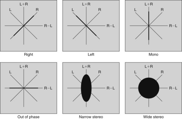
One disadvantage of the polar display methodology is that, in the absence of modulation, the cathode ray will remain undeviated and a bright spot will appear at the center of the display, gradually burning a hole on the phosphor! To avoid this, commercial polar displays incorporate cathode modulation (k mod) so that, if the signal goes below a certain value, the cathode is biased until the anode current cuts off, extinguishing the beam.

27.3. Standard Operating Levels and Line-Up Tones

Irrespective of the type of meter employed, it should be pretty obvious that a meter is entirely useless unless it is calibrated in relation to a particular signal level (think about it if rulers had different centimeters marked on them!).

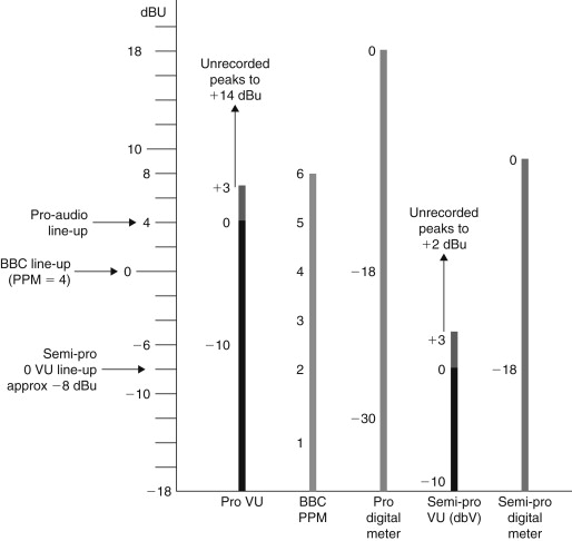
Three important line-up levels exist (see Figure 27.6):

• PPM4=0 dBu=0.775 V rms, used by United Kingdom broadcasters.
• 0VU=+4 dBu=1.23 V rms, used in commercial music sector.
• 0VU=−10 dBV=316 mV rms, used in consumer and “prosumer” equipment.

Figure 27.6. Standard levels compared.

27.4. Digital Line-Up

The question of how to relate 0 VU and PPM 4 to a digital maximum level of 0 dBFS (for 0 dB relative to full scale) has been the topic of hot debate. Fortunately, the situation has crystallized over the last few years to the extent that it is now possible to describe the situation on the basis of widespread implementation in the United States and with European broadcasters. Essentially,

• 0 VU=+4 dBu=−20 dBFS (SMPTE RP155)
• PPM4=0 dBu=−18 dBFS (EBU R64-1992)

Sadly, these recommendations are not consistent. And while the EBU recommendation seems a little pessimistic in allowing extra 4-dB headroom above their own worst-case scenario, the SMPTE suggestion looks positively gloomy in allowing 20 dB above the alignment level. Although this probably reflects the widespread, although technically incorrect, methodology, when monitoring with VUs, of setting levels so that peaks often drive the meter well into the red section.

27.5. Sound Mixer Architecture and Circuit Blocks

The largest, most expensive piece of capital electronic equipment in any professional studio is the main studio mixer. So much so that in publicity shots of a recording studio this component is always seen to dominate the proceedings! Perhaps that’s why there seem to be so many terms for it: mixer, mixing desk, or just desk, audio console, console, and simply “the board,” to name but a few. To many people outside of the recording industry, the audio mixer represents the very essence of sound recording. This is partially correct, for it is at the console that many of the important artistic decisions that go toward mixing a live band or a record are made. However, in engineering terms, this impression is misleading. The audio console is a complicated piece of equipment but, in its electronic essence, its duties are relatively simple. In other words, the designer of an audio mixer is more concerned with the optimization of relatively simple circuits, which may then be repeated many, many times, than he/she is with the design of clever or imaginative signal processing. But before we investigate the individual circuit elements of an audio mixer, it is important to understand the way in which these blocks fit together. This is usually termed system architecture.

27.5.1. System Architecture

There is no simple description of audio console system architecture. That’s because there exist different types of consoles for different duties and because every manufacturer (and there are very many of them) each has their own ideas about how best to configure the necessary features in a manner that is operationally versatile, ergonomic, and maintains the “cleanest” signal path from input to output. However, just as houses all come in different shapes and sizes and yet all are built relying upon the same underlying assumptions and principles, most audio mixers share certain system topologies.

27.5.2. Input Strip

The most conspicuous “building block” in an audio console, and the most obviously striking at first glance, is the channel input strip. Each mixer channel has one of these and they tend to account for the majority of the panel space in a large console. A typical input strip for a small recording console is illustrated in Figure 27.9. When you consider that a large console may have 24, 32, or perhaps 48 channels—each a copy of the strip illustrated in Figure 27.9—it is not surprising that large commercial studio consoles look so imposing. But always remember, however “frightening” a console looks, it is usually only the sheer bulk that gives this impression. Most of the panel is repetition and once one channel strip is understood, so are all the others!

Much harder to fathom, when faced with an unfamiliar console, are the bus and routing arrangements that feed the group modules, the monitor, and master modules. These “hidden” features relate to the manner in which each input module may be assigned to the various summing amplifiers within the console. And herein lies the most important thing to realize about a professional audio console; that it is many mixers within one console. First let’s look at the groups.

27.5.3. Groups

Consider mixing a live rock band. Assume that it is a quintet: a singing bass player, one guitarist, a keyboard player, a saxophonist, and a drummer. The inputs to the mixer might look something like this:

Table 27.2.

Channel 1	Vocal mic
Channel 2	Bass amp mic
Channel 3	Lead guitar amp mic
Channel 4	Backing mic (for keyboardist)
Channel 5	Backing mic (for second guitarist)
Channel 6	Sax mic
Channel 7	Hi-hat mic
Channel 8	Snare mic
Channel 9	Bass drum mic
Channels 10 and 11	Drum overheads
Channels 12 and 13	Stereo line piano input
Channels 14 and 15	Sound module line input

Clearly inputs 7 to 11 are all concerned with the drums. Once these channels have been set so as to give a good balance between each drum, it is obviously convenient to group these faders together so that the drums can be adjusted relative to the rest of the instruments. This is the role of the separate summing amplifiers in a live console, to group various instruments together. That’s why these smaller “mixers within mixers” are called groups. These group signals are themselves fed to the main stereo mixing amplifier, the master section. Mixer architecture signal flow is therefore channeled to groups and groups to master output mixer, as shown in Figure 27.7. A block schematic of a simplified live-music mixer is given in Figure 27.8 in which this topology is evident.

Figure 27.7. Signal flow.

Figure 27.8. Schematic of a live-music console.

27.5.4. Pan Control

Stereophonic reproduction from loudspeakers requires that stereo information is carried by interchannel intensity differences alone, as there is no requirement for interchannel delay differences. The pan control progressively attenuates one channel while progressively strengthening the other as the knob is rotated, with the input being shared equally between both channels when the knob is in its center (12 o’clock) position. In the sound mixer shown in Figure 27.8, note that the channel pan control operates in a rather more flexible manner, as a control that may be used to “steer” the input signal between either of the pairs of buses selected by the routing switches. The flexibility of this approach becomes evident when a console is used in a multitrack recording session.

27.5.5. Effect Sends and Returns

Not all the functions required by the balance engineer can be incorporated within the audio mixer. To facilitate the interconnection with outboard equipment, most audio mixers have dedicated mix amplifiers and signal injection points called effect sends and returns, which make incorporation of other equipment within the signal flow as straightforward as possible.

27.5.6. The Groups Revisited

In a recording situation, the mixing groups may well ultimately be used in the same manner as described in relation to the live console, to group sections of the arrangement so as to make the task of mixing more manageable. But the groups are used in a totally different way during recording or tracking. During this phase, the groups are used to route signals to the tracks of the multitrack tape machine. From an electronic point of view, the essential difference here is that, in a recording situation, the group outputs are utilized directly as signals and a recording mixer must provide access to these signals. Usually a multitrack machine is wired so that each group output feeds a separate track of the multitrack tape recorder. Often there are not enough groups to do this, in which case, each group feeds a number of tape machine inputs, usually either adjacent tracks or in “groups of groups” so that, for instance, groups 1 to 8 will feed inputs 1 to 8 and 9 to 16 and so on.

27.5.7. The Recording Console

So far, this is relatively straightforward. But a major complication arises during the tracking of multitrack recordings because not only must signals be routed to the tape recorder via the groups, tape returns must be routed back to the mixer to guide the musicians as to what to play next. And this must happen at the same time! In fact, it is just possible for a good sound engineer, using “crafty” routing, to cope with this using a straightforward live mixing desk. But it is very difficult. What is really required is a separate mixer to deal with the gradually increasing numbers of tape replay returns, thereby keeping the main mixer free for recording duties. Various mixer designers have solved this problem in different ways. Older consoles (particularly of English origin) have tended to provide an entirely separate mixer (usually to the right of the group and main faders) devoted to dealing with the return signals. Such a mixer architecture is known as a split console. The alternative approach, which is now very widespread, is known as the in-line console, so named because the tape-return controls are embedded within each channel strip, in line with the main fader. This is the type of console considered in detail later. From an electronic point of view, very little difference exists between these approaches; the difference is more one of operational philosophy and ergonomics.

Both the split and in-line console are yet another example of a “mixer within a mixer.” In effect, in the in-line console, the tape returns feed an entirely separate mixer so that each tape return signal travels via a separate fader (sometimes linear, sometimes rotary) and pan control before being summed on an ancillary stereo mix bus known as the monitor bus. The channel input strip of an in-line console is illustrated in Figure 27.9. The monitor bus is exceptionally important in a recording console because it is the output of this stereo mix amplifier that supplies the signal that is fed to the control room power amplifier during the tracking phase of the recording process. (Usually, control room outputs are explicitly provided on the rear panels of a recording console for this purpose.) The architecture is illustrated in Figure 27.10. During mixdown, the engineer will want to operate using the main faders and pan controls, because these are the most operationally convenient controls, being closest to the mixer edge nearest the operator. To this end, the in-line console includes the ability to switch the tape returns back through the main input strip signal path, an operation known as “flipping” the faders. The circuitry for this is illustrated in Figure 27.11.

Figure 27.9. Input strip of an in-line console.

Figure 27.10. In-line console architecture.

Figure 27.11. Fader “flip” mechanism.

27.5.8. Talkback

Talkback exists so that people in the control room are able to communicate with performers in the studio. So as to avoid sound “spill” from the loudspeaker into open microphones (as well as to minimize the risk of howl-round), performers inside the studio invariably wear headphones and therefore need a devoted signal that may be amplified and fed to special headphone amplifiers. In the majority of instances this signal is identical to the signal required in the control room during recording (i.e., the monitor bus). In addition, a microphone amplifier is usually provided within the desk, which is summed with the monitor bus signal and fed to the studio headphone amplifiers. This microphone amplifier is usually energized by a momentary switch to allow the producer or engineer to communicate with the singer or instrumentalist, but which cannot, thereby, be left open, thus distracting the singer or allowing them to hear a comment in the control room that may do nothing for their ego!

27.5.9. Equalizers

For a variety of reasons, signals arriving at the recording console may require spectral modification. Sometimes this is due to the effect of inappropriate microphone choice or of incorrect microphone position. Sometimes it is due to an unfortunate instrumental tone (perhaps an unpleasant resonance). Most often, the equalizer (or simply EQ) is used in a creative fashion to enhance or subdue a band (or bands) of frequencies so as to blend an instrument into the overall mix or boost a particular element so that its contribution is more incisive.

It is this creative element in the employment of equalization that has created the situation that exists today, that the quality of the EQ is often a determining factor in a recording engineer’s choice of one console over another. The engineering challenges of flexible routing, low interchannel cross talk, low noise, and good headroom having been solved by most good manufacturers, the unique quality of each sound desk often resides in the equalizer design. Unfortunately, this state of affairs introduces a subjective (even individualistic) element into the subject of equalization, which renders it very difficult to cover comprehensively. Sometimes it seems that every circuit designer, sound engineer, and producer each has his, or her, idea as to what comprises an acceptable, an average, and an excellent equalizer! A simple equalizer section—and each control’s effect—is illustrated in Figure 27.12.

Figure 27.12. Equalizer controls.

27.6. Audio Mixer Circuitry

Now that we understand the basic architecture of the mixer, it is time to look at each part again and understand the function of the electrical circuits in each stage in detail.

The input strip is illustrated in Figure 27.9. Note that below the VU meter, the topmost control is the channel gain trim. This is usually switchable between two regimes: a high gain configuration for microphones and a lower gain line level configuration. This control is set with reference to its associated VU meter. Below the channel gain are the equalization controls; the operation of these controls is described in detail later.

27.6.1. Microphone Preamplifiers

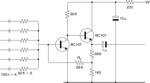
Despite the voltage amplification provided by a transformer or preamplifier, the signal leaving a microphone is still, at most, only a few millivolts. This is much too low a level to be suitable for combining with the outputs of other microphones inside an audio mixer. So, the first stage of any audio mixer is a so-called microphone preamplifier, which boosts the signal entering the mixer from the microphone to a suitable operating level. The example given here is taken from a design (Brice, 1990), which was for a portable, battery-driven mixer—hence the decision to use discrete transistors rather than current-thirsty op-amps. Each of the input stage microphone amplifiers is formed of a transistor “ring of three.” The design requirement is for good headroom and a very low noise figure. The final design is illustrated in Figure 27.13.^[1] The current consumption for each microphone preamplifier is less than 1 mA.

¹ The amplifier shown has an input noise density of 3 nV per root hertz and a calculated input noise current density of 0.3 pA per root hertz ignoring flicker noise. The frequency response and the phase response remain much the same regardless of gain setting. This seems to go against the intractable laws of gain-bandwidth product: as we increase the gain we must expect the frequency response to decrease and vice versa. In fact, the ring-of-three circuit is an early form of “current-mode-feedback” amplifier, which is currently very popular in video applications. The explanation for this lies in the variable gain-setting resistor R^a. This not only determines the closed-loop gain by controlling the proportion of the output voltage fed back to the inverting port but it also forms the dominating part of the emitter load of the first transistor and consequently the gain of the first stage. As the value of R^a decreases, so the feedback diminishes and the closed-loop gain rises. At the same time, the open-loop gain of the circuit rises because TR1's emitter load falls in value. Consequently the performance of the circuit in respect of phase and frequency response, and consequently stability, remains consistent regardless of gain setting.

Figure 27.13. Microphone preamplifier.

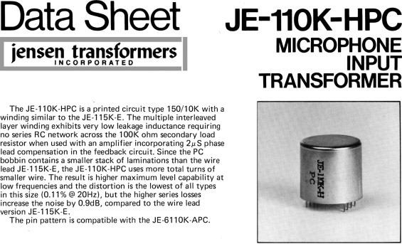
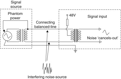
For more demanding studio applications, a more complex microphone preamplifier is demanded. First, the stage illustrated in Figure 27.13 is only suitable for unbalanced microphones, and the majority of high-quality microphones utilize balanced connection, as they are especially susceptible to hum pick-up if this type of circuit is not employed. Second, high-quality microphones are nearly always capacitor types and therefore require a polarizing voltage to be supplied for the plates and for powering the internal electronics. This supply (known as phantom power as mentioned earlier) is supplied via the microphone’s own signal leads and must therefore be isolated from the microphone preamplifier. This is one area where audio transformers (Figure 27.14) are still used, and an example of a microphone input stage using a transformer is illustrated, although plenty of practical examples exist where transformerless stages are used for reasons of cost.

Figure 27.14. Microphone transformer.

Figure 27.15. Transformer-based input stage.

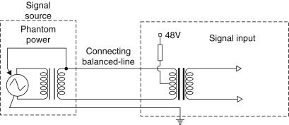
Note that the phantom power is provided via resistors, which supply both phases on the primary side of the transformer, with the current return being via the cable screen. The transformer itself provides some voltage gain at the expense of presenting a much higher output impedance to the following amplifier. However, the amplifier has an extremely high input impedance (especially so when negative feedback is applied) so this is really of no consequence. In Figure 27.14, amplifier gain is made variable so as to permit the use of a wide range of microphone sensitivities and applications. An ancillary circuit is also provided that enables the signal entering the circuit to be attenuated by 20 dB, which allows for very high output microphones without overloading the electronics.

27.6.2. Insert Points

After the channel input amplifier, insert points are usually included. These allow external (outboard) equipment to be patched into the signal path. Note that this provision is usually via jack connectors, which are normalized when no plug is inserted (Figure 27.16).

Figure 27.16. Insert points.

27.6.3. Equalizers and Tone Controls

At the very least, a modern recording console provides a basic tone-control function on each channel input, like that shown in Figure 27.17. This circuit is a version of the classic circuit due to Baxandall. However, this type of circuit only provides a fairly crude adjustment of bass and treble ranges, as illustrated in Figure 27.12. This type of response (for fairly obvious reasons) is often termed a “shelving” equalizer. So, the Baxandall shelving EQ is invariably appended with a midfrequency equalizer, which is tunable over a range of frequencies, thereby enabling the sound engineer to adjust the middle band of frequencies in relation to the whole spectrum (see also Figure 27.12). A signal manipulation of this sort requires a tuned circuit, which is combined within an amplifier stage, which may be adjusted over a very wide range of attenuation and gain (perhaps as much as ±20 dB). How such a circuit is derived is illustrated in Figure 27.18.

Figure 27.17. A simple tone control circuit.

Figure 27.18(a–c). Derivation of midband parametric EQ circuit; see text.

Imagine that Z1 is a small resistance. When the slider of VR1 is at position A, the input is heavily attenuated and the lower feedback limb of the op-amp is at its greatest value (i.e., the gain of the stage is low). Now imagine moving the slider of VR1 position B. The situation is reversed; the input is much less attenuated and the gain of the amplifier stage is high. This circuit therefore acts as a gain control because point A is arranged to be at the extreme anticlockwise position of the control. As a tone control this is obviously useless. However, in the second part of Figure 27.18(b), Z1 is replaced with a tunable circuit, formed by a variable inductor and a capacitor. This tuned circuit has high impedance—and therefore little effect—except at its resonant frequency, whereupon it acquires very low dynamic impedance. With the appropriate choice of inductor and capacitor values, the midfrequency equalizer can be made to operate over the central frequency range. The action of VR1 is to introduce a bell-shaped EQ response (as illustrated in Figure 27.12), which may be used to attenuate or enhance a particular range of frequencies, as determined by the setting of the variable inductor.

27.6.4. Inductor–Gyrators

As shown, the frequency adaptive component is designated as a variable inductor. Unfortunately, these components do not exist readily at audio frequencies and to construct components of this type expressly for audio frequency equalization would be very expensive. For this reason, the variable inductors in most commercial equalizers are formed by gyrators—circuits that emulate the behavior of inductive components by means of active circuits, which comprise resistors, capacitors, and op-amps. An inductor–gyrator circuit is illustrated in Figure 27.18(c). This is known as the “bootstrap” gyrator and its equivalent circuit is also included within the figure. Note that this type of gyrator circuit (and indeed most others) presents a reasonable approximation to an inductor that is grounded at one end. Floating inductor–gyrator circuits do exist but are rarely seen.

Operation of the bootstrap gyrator circuit can be difficult to visualize, but think about the two frequency extremes. At low frequencies, C^a will not pass any signal to the input of the op-amp. The impedance presented at point P will therefore be the output impedance of the op-amp (very low) in series with R^b, which is usually designed to be in the region of a few hundred ohms. Just like an inductor, the reactance is low at low frequencies. Now consider the high-frequency case. At HF, C^a will pass signal so that the input to the op-amp will be substantially that presented at point P. Because the op-amp is a follower, the output will be a low-impedance copy of its input. By this means, resistor R^b will thereby have little or no potential across it because the signal at both its ends is the same. Consequently, no signal current will pass through it. In engineering slang, the low-value resistor R^b is said to have been “bootstrapped” by the action of the op-amp and therefore appears to have a much higher resistance than it actually has. Once again, just like a real inductor, the value of reactance at high frequencies at point P is high. The inductor–gyrator circuit is made variable by the action of R^a, which is formed by a variable resistor component. This alters the breakpoint of the RC circuit C^a/R^a and thereby the value of the “virtual” inductor.

In recent years, the fascination in “retro” equipment has brought about a resurgence of interest in fixed inductor–capacitor type equalizers. Mostly outboard units, these are often passive EQ circuits [often of great complexity, as illustrated in Figure 27.18(d)], followed by a valve line amplifier to make up the signal gain lost in the EQ. In a classic LC-type equalizer, the variable-frequency selection is achieved with switched inductors and capacitors.

Figure 27.18(d). Older, passive equalizer circuit.

27.6.5. ‘Q’

Often it is also useful to control the Q of the resonant circuit so that a very broad, or a very narrow, range of frequencies can be affected as appropriate. Hence the inclusion of the Q control as shown in Figure 27.12. This effect is often achieved by means of a series variable resistor in series with the inductor–capacitor (or gyrator–capacitor) frequency-determining circuit.

27.6.6. Effect Send and Return

The effect send control feeds a separate mix amplifier. The output of this submix circuit is made available to the user via an effect send output on the back of the mixer. An effect return path is also usually provided so that the submix (suitably “effected”—usually with digital reverberation) can be reinjected into the amplifier at line level directly into the main mix amplifiers.

27.6.7. Faders and Pan Controls

Beneath the effect send control is the pan control and the main fader. Each channel fader is used to control the contribution of each channel to the overall mix as described earlier. A design for a fader and pan pot is illustrated in Figure 27.19. The only disadvantage of the circuit is that it introduces loss. However, its use is confined to a part of the circuit where the signal is at a high level and the Johnson noise generated in the network is very low since all the resistances are low. The circuit takes as its starting point that a semilog audio-taper fader can be obtained using a linear potentiometer when its slider tap and “earthy” end is shunted with a resistor one-tenth of the value of the total potentiometer resistance. Resistors R^c and R^d and VR^a, the pan pot itself, form this one-tenth value network. Because the slider of the pan pot is grounded and the output signal is obtained from either end of the pan pot, it is clear that in either extreme position of VR^a, all the signal will appear on one channel and none on the other. It is then only a matter of deciding whether the control law of the pan pot is of the correct type. The calculation of the control law obtained from the circuit is complicated because the signal level fed to left and right channels is not proportional to the resistive value of each part of VR^a. This is because the total value of the network R^c, R^d, and VR^a, although reasonably constant, is not the same irrespective of the setting of VR^a and so the resistive attenuator comprising the top part of VR^b and its lower part, shunted by the pan pot network, is not constant as VR^a is adjusted. Furthermore, as VR^a is varied, so the output resistance of the network changes and, since this network feeds a virtual-earth summing amplifier, this effect also has an influence on the signal fed to the output because the voltage-to-current converting resistor feeding the virtual-earth node changes value. The control law of the final circuit is nonlinear: the sum of left and right, when the source is positioned centrally, adding to more than the signal appearing in either channel when the source is positioned at an extreme pan position. This control law is very usable with a source seeming to retain equal prominence as it is “swept across” the stereo stage.

Figure 27.19. Fader and pan pot circuit.

27.6.8. Mix Amplifiers

The mix amplifier is the core of the audio mixer. It is here that the various audio signals are combined together with as little interaction as possible. The adoption of the virtual-earth mixing amplifier is universal. An example of a practical stereo mix amplifier is shown in Figure 27.20. Here, the summing op-amp is based on a conventional transistor pair circuit. The only difficult decision in this area is the choice of the value for R^b. It is this value, combined with the input resistors, that determines the total contribution each input may make to the final output.

Figure 27.20. Mix amplifier.

27.6.9. Line-Level Stages

Line-level audio stages are relatively straightforward. Signals are at a high level, so noise issues are rarely encountered. The significant design parameters are linearity, headroom, and stability. Another issue of some importance is signal balance, at least in professional line-level stages, which are always balanced. Of these, output-stage stability is the one most often ignored by novice designers.

A high degree of linearity is achieved in modern line-level audio stages by utilizing high open-loop gain op-amps and very large feedback factors. The only issue remaining, once the choice of op-amp has been made, is available headroom. This is almost always determined by choice of power supply rails. Taking a typical audio op-amp (TL072, for example), maximum output swing is usually limited to within a few volts of either rail. So, furnished with 12-V positive and negative supplies, an op-amp could be expected to swing 18 Vpk-pk. This is equivalent to 6.3 V rms, or 16 dBV, easily adequate then for any circuit intended to operate at 0 VU=−10 dBV. In a professional line-output circuit, like that shown in Figure 27.21, this voltage swing is effectively doubled because the signal appears “across” the two opposite phases. The total swing is therefore 12.6 V rms, which is equivalent to 24 dBu. For equipment intended to operate at 0 VU=+4 dBu, such a circuit offers 20 dB headroom, which is adequate. However, ±12-V supplies really represent the lowest choice of rail volts for professional equipment and some designers prefer to use 15-V supplies for this very reason.

Figure 27.21. Line output circuit.

Looking again at the output stage circuit illustrated in Figure 27.21, note the inclusion of the small value resistors in the output circuit of the op-amps. These effectively add some real part to the impedance “seen” by the op-amp when it is required to drive a long run of audio cables. At audio frequencies, the equipment interconnection cable looks to the output stage as a straightforward—but relatively large—capacitance. Also, a large negative reactance is, almost always, an excellent way to destabilize output circuits. Output “padding” resistors, such as R132 and R133, help a great deal in securing a stable performance into real loads.

Line-level input stages present different problems. Note that the function performed by the circuit in Figure 27.21, over and above its duty to drive the output cables, is to derive an equal and opposite signal so as to provide a balanced audio output from a single-ended, unbalanced input signal. This is a common feature of professional audio equipment because, although balanced signals are the norm outside the equipment, internally most signals are treated as single ended. The reasons for this are obvious; without this simplification all the circuitry within, for example, a console would be twice as complex and twice as expensive.

The line-level input stage on professional equipment therefore has to perform a complementary function to the output stage to derive a single-ended signal from the balanced signal presented to the equipment. Conceptually, the simplest circuit is a transformer, like that shown in Figure 27.22. In many ways this is an excellent solution for the following reasons: it provides electrical isolation, it has low noise and distortion, and it provides good headroom, provided the core doesn’t saturate. But, most important of all, it possesses excellent common-mode rejection (CMR). That means that any signal that is common (i.e., in phase) on both signal phases is rejected and does not get passed on to following equipment. By contriving the two signal conductors within the signal cable to occupy—as nearly as possible—the same place, by twisting them together, any possible interference signal is induced equally in both phases. Such a signal thereafter cancels in the transformer stage because a common signal cannot cause a current to flow in the primary circuit and cannot, therefore, cause one to flow in the secondary circuit. This is illustrated in Figure 27.22 as well.

Figure 27.22. Balanced input circuit, and CM rejection.

Another advantage of a balanced signal interface is that the signal circuit does not include ground. It thereby confers immunity to ground-sourced noise signals. On a practical level it also means that different equipment chassis can be earthed, for safety reasons, without incurring the penalty of multiple signal return paths and the inevitable “hum loops” this creates. However, transformers are not suitable in many applications for a number of reasons. First, they are very expensive. Second, they are heavy, bulky, and tend to be microphonic (i.e., they have a propensity to transduce mechanical vibration into electrical energy!) so that electronically balanced input stages are widely employed instead. These aim to confer all the advantages of a transformer cheaply, quietly, and on a small scale. To some degree, an electronic stage can never offer the same degree of CMR, as well as the complete galvanic isolation, offered by a transformer.

27.7. Mixer Automation

Mixer automation consists (at its most basic level) of computer control over the individual channel faders during a mixdown. Even the most dexterous and clear thinking balance engineer obviously has problems when controlling perhaps as many as 24 or even 48 channel faders at once. For mixer automation to work, several things must happen. First, the controlling computer must know precisely which point in the song or piece has been reached in order that it can implement the appropriate fader movements. Second, the controlling computer must have, at its behest, hardware that is able to control the audio level on each mixer channel, swiftly and noiselessly. This last requirement is fulfilled a number of ways, but most often a voltage-controlled amplifier (VCA) is used.

A third requirement of a fader automation system is that the faders must be “readable” by the controlling computer so that the required fader movements can be implemented by the human operator and memorized by the computer for subsequent recall.

A complete fader automation system is shown in schematic form in Figure 27.23. Note that the fader does not pass the audio signal at all. Instead the fader simply acts as a potentiometer driven by a stabilized supply. The slider potential now acts as a control voltage, which could, in theory, be fed directly to the voltage-controlled amplifier, VCA1. But this would miss the point. By digitizing the control voltage, and making this value available to the microprocessor bus, the fader “position” can be stored for later recall. When this happens, the voltage (at the potentiometer slider) is recreated by means of a DAC and this is applied to the VCA, thereby reproducing the operator’s original intentions.

Figure 27.23. Fader automation system.

One disadvantage of this type of system is the lack of operator feedback once the fader operation is overridden by the action of the VCA; importantly, when in recall mode, the faders fail, by virtue of their physical position, to tell the operator (at a glance) the condition of any of the channels and their relative levels. Some automation systems attempt to emulate this important visual feedback by creating an iconic representation of the mixer on the computer screen. Some even allow these virtual faders to be moved, on screen, by dragging them with a mouse. Another more drastic solution, and one that has many adherents on sound quality grounds alone, is to use motorized faders as part of the control system. In this case the faders act electrically as they do in a nonautomated mixer, carrying the audio signal itself. The control system loop is restricted to reading and “recreating” operator fader physical movements. Apart from providing unrivalled operator feedback (and the quite thrilling spectacle of banks of faders moving as if under the aegis of ghostly hands!), the advantage of this type of automation system is the lack of VCAs in the signal path. VCA circuits are necessarily complicated and their operation is beset with various deficiencies, mostly in the areas of insufficient dynamic range and control signal breakthrough. These considerations have kept motorized faders as favorites among the best mixer manufacturers, despite their obvious complexity and cost.

27.7.1. Time Code

Time code is the means by which an automation system is kept in step with the music recorded onto tape. Normally, a track of the multitrack tape is set aside from audio use and is devoted to recording a pseudo audio signal composed of a serial digital code.

27.8. Digital Consoles

27.8.1. Introduction to Digital Signal Processing (DSP)

DSP involves the manipulation of real-world signals (for instance, audio signals, video signals, medical or geophysical data signals) within a digital computer. Why might we want to do this? Because these signals, once converted into digital form (by means of an analogue to digital converter), may be manipulated using mathematical techniques to enhance, change, or display data in a particular way. For instance, the computer might use height or depth data from a geophysical survey to produce a colored contour map or the computer might use a series of two-dimensional medical images to build up a three-dimensional virtual visualization of diseased tissue or bone. Another application, this time an audio one, might be used to remove noise from a music signal by carefully measuring the spectrum of the interfering noise signal during a moment of silence (for instance, during the run-in groove of a record) and then subtracting this spectrum from the entire signal, thereby removing only the noise—and not the music—from a noisy record.

DSP systems have been in existence for many years, but, in these older systems, the computer might take many times longer than the duration of the signal acquisition time to process the information. For instance, in the case of the noise reduction example, it might take many hours to process a short musical track. This leads to an important distinction that must be made in the design, specification, and understanding of DSP systems; that of nonreal time (where the processing time exceeds the acquisition or presentation time) and real-time systems, which complete all the required mathematical operations so fast that the observer is unaware of any delay in the process. When we talk about DSP in digital audio it is always important to distinguish between real-time and nonreal-time DSP. Audio outboard equipment that utilizes DSP techniques is, invariably, real time and has dedicated DSP chips designed to complete data manipulation fast. Nonreal-time DSP is found in audio processing on a PC or Apple Mac where some complex audio tasks may take many times the length of the music sample to complete.

27.8.2. Digital Manipulation

So, what kind of digital manipulations might we expect? Let’s think of the functions that we might expect to perform within a digital sound mixer. First, there is addition. Clearly, at a fundamental level, that is what a mixer is—an “adder” of signals. Second, we know that we want to be able to control the gain of each signal before it is mixed. So multiplication must be needed too. So far, the performance of the digital signal processing “block” is analogous with its analogue counterpart. The simplest form of digital audio mixer is illustrated in Figure 27.24. In this case, two digital audio signals are each multiplied by coefficients (k1 and k2) derived from the position of a pair of fader controls; one fader assigned to either signal. Signals issuing from these multiplication stages are subsequently added together in a summing stage. All audio mixers possess this essential architecture, although it may be supplemented many times over.

Figure 27.24. Simple digital audio mixer.

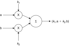
But, in fact, the two functions of addition and multiplication, plus the ability to delay signals easily within digital systems, allow us to perform all the functions required within a digital sound mixer, even the equalization functions. That’s because equalization is a form of signal filtering on successive audio samples, which is simply another form of mathematical manipulation, even though it is not usually regarded as such in analogue circuitry.

27.8.3. Digital Filtering

The simplest form of analogue low-pass filter is shown in Figure 27.25. Its effect on a fast rise-time signal wave front (an “edge”) is also illustrated. Note that the resulting signal has its “edges” slowed down in relation to the incoming signal. Its frequency response is also illustrated, with its turnover frequency. Unfortunately, in digital circuits there are no such things as capacitors or inductors, which may be used to change the frequency response of a circuit. However, if you remember, we’ve come across situations before in sections as diverse as microphones to flanging, phasing, and chorus wherein a frequency response was altered by the interaction of signals delayed with respect to one another. This principle is the basis behind all digital filtering and may be extended to include several stages of delay as shown in Figure 27.26. By utilizing a combination of adder and variable multiplication factors (between the addition function and the signal taps) it is possible to achieve a very flexible method of signal filtering in which the shape of the filter curve may be varied over a very wide range of shapes and characteristics. While such a technique is possible in analogue circuitry, note that the “circuit” (shown in Figure 27.26) is actually not a real circuit at all, but a notional block diagram. It is in the realm of digital signal processing that such a filtering technique really comes into its own: the DSP programmer has only to translate these processes into microprocessor type code to be run on a microcontroller IC, which is specifically designed for audio applications—a so-called DSP IC. Herein lies the greatest benefit of digital signal processing—that by simply reprogramming the coefficients in the multiplier stages, a completely different filter may be obtained. Not only that, but if this is done in real time too, the filter can be made adaptive, adjusting to demands of the particular moment in a manner that might be useful for signal compression or noise reduction.

Figure 27.25. RC low-pass filter.

Figure 27.26. Principle of a digital filter.

27.8.4. Digital Mixer Architecture

Because of the incredible flexibility and “programmability” of digital signal processing-based mixers, architecture is much harder (less necessary!) to define. This, alone, is a great advantage. For instance, digital processing too has blurred the traditional distinction between split and in-line consoles because, with the aid of configurable signal paths and motorized faders, the same small group of faders can be used to “flip” between the role of the recording mixer and that of the playback mixer.

Box 27.1. Fact Sheet #12: Digital signal processing

• Architecture of DSP devices
• Convolution
• Impulse response
• FIR and IIR digital filters
• Design of digital filters
• Frequency response
• Derivation of band-pass and high-pass filters
• Digital frequency domain analysis—the z-transform
• Problems with digital signal processing

Architecture of DSP devices

The first computers, including those developed at Harvard University, had separate memory space for program and data; this topology being known as Harvard architecture. In fact, the realization, by John von Neumann—the Hungarian-born mathematician—that program instructions and data were only numbers and could share the same “address space” was a great breakthrough at the time and was sufficiently radical that this architecture is often named after its inventor. The advantage of the von Neumann approach was great simplification but at the expense of speed because the computer can only access either an instruction or data in any one processing clock cycle. The fact that virtually all computers follow this latter approach illustrates that this limitation is of little consequence in the world of general computing.

However, the speed limitation “bottleneck,” inevitable in the von Neumann machine, can prove to be a limitation in specialist computing applications such as digital audio signal processing. As we have seen in the case of digital filters, digital signal processing contains many, many multiply and add type instructions of the form

Unfortunately, a von Neumann machine is really pretty inefficient at this type of calculation so the Harvard architecture lives on in many DSP chips, meaning that a multiply and add operation can be performed in one clock cycle; this composite operation is termed a Multiply ACcumulate (MAC) function. A further distinction pertains to the incorporation within the DSP IC of special registers that facilitate the managing of circular buffers for the implementation of reverb, phasing, chorus, and flanging effects.

The remaining differences between a DSP device and a general purpose digital microcomputer chip relate to the provision of convenient interfaces, thereby allowing direct connection of ADCs, DACs, and digital transmitter and receiver ICs.

Convolution

In the simple three-stage digital filter, we imagined the step function being multiplied by a quarter, then by a half, and finally by a quarter again; at each stage, the result was added up to give the final output. This actually rather simple process is given a frightening name in digital signal processing theory, where it is called convolution.

Discrete convolution is a process that provides a single output sequence from two input sequences. In the example given earlier, a time-domain sequence—the step function—was convolved with the filter response yielding a filtered output sequence. In textbooks, convolution is often denoted by the character ^‘*’. So if we call the input sequence h(k) and the input sequence x(k), the filtered output would be defined as

Impulse response

A very special result is obtained if a unique input sequence is convolved with the filter coefficients. This special result is known as the filter’s impulse response, and the derivation and design of different impulse responses are central to digital filter theory. The special input sequence used to discover a filter’s impulse response is known as the “impulse input.” (The filter’s impulse response being its response to this impulse input.) This input sequence is defined to be always zero, except for one single sample, which takes the value 1 (i.e., the full-scale value). We might define, for practical purposes, a series of samples like this

0, 0, 0, 0, 0, 1, 0, 0, 0, 0

Now imagine these samples being latched through the three-stage digital filter shown earlier. The output sequence will be

0, 0, 0, 0, 0, 1/4, 1/2, 1/4, 0, 0, 0, 0

Obviously the zeros don’t really matter, what’s important is the central section: 1/4, 1/2, 1/4. This pattern is the filter’s impulse response.

FIR and IIR digital filters

Note that the impulse response of the aforementioned filter is finite: in fact, it only has three terms. So important is the impulse response in filter theory that this type of filter is actually defined by this characteristic of its behavior and is named a finite impulse response (FIR) filter. Importantly, note that the impulse response of an FIR filter is identical to its coefficients.

Now look at the digital filter in Figure F27.1. This derives its result from both the incoming sequence and from a sequence that is fed back from the output. Now if we perform a similar thought experiment to the convolution example given earlier and imagine the resulting impulse-response from a filter of this type, it results in an output sequence like that illustrated in the figure: that’s to say, an infinitely decaying series of values. Once again, so primordial is this characteristic that this category of filter is termed an infinite impulse response (IIR) filter.

Figure F27.1. Infinite impulse response filter.

IIR filters have both disadvantages and advantages over the FIR type. First, they are very much more complicated to design because their impulse response is not simply reflected by the tap coefficients, as in the FIR. Second, it is in the nature of any feedback system (like an analogue amplifier) that some conditions may cause the filter to become unstable if it is has not been thoroughly designed, simulated, and tested. Furthermore, the inherent infinite response may cause distortion and/or rounding problems as calculations on smaller and smaller values of data are performed. Indeed, it’s possible to draw a parallel between IIR filters and analogue filter circuits: they share the disadvantages of complexity of design and possible instability and distortion, but they also share the great benefit that they are efficient. An IIR configuration can be made to implement complex filter functions with only a few stages, whereas the equivalent FIR filter would require many hundreds of taps with all the drawbacks of cost and signal delay that this implies. (Sometimes FIR and IIR filters are referred to as “recursive” and “nonrecursive,” respectively; these terms directly reflect the filter architecture.)

Design of digital filters

Digital filters are nearly always designed from knowledge of the required impulse response. IIR and FIR filters are both designed in this way, although the design of IIR filters is complicated because the coefficients do not represent the impulse response directly. Instead, IIR design involves various mathematical methods, which are used to analyze and derive the appropriate impulse response from the limited number of taps. This makes the design of IIR filters from first principles rather complicated and math heavy! Fortunately, FIRs are easier to understand, and a brief description gives a good deal of insight into the design principles of all digital filters.

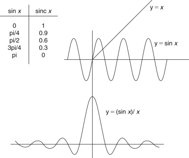
We already noted that the response type of the 1/4, 1/2, 1/4 filter was a low-pass; remember it “slowed down” the fast rising edge of the step waveform. If we look at the general form of this impulse response, we will see that this is a very rough approximation to the behavior of an ideal low-pass filter in relation to reconstruction filters. There we saw that the (sin x)/x function defines the behavior of an ideal, low-pass filter and the derivation of this function is given in Figure F27.2. Sometimes termed a sinc function, it has the characteristic that it is infinite, gradually decaying with ever smaller oscillations about zero. This illustrates that the perfect low-pass FIR filter would require an infinite response, an infinite number of taps and the signal would take an infinitely long time to pass through it! Fortunately for us, we do not need such perfection.

Figure F27.2. Derivation of sin x/x function.

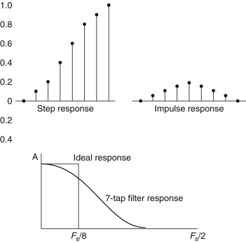
However, the 1/4, 1/2, 1/4 filter is really a very rough approximation indeed. So let’s now imagine a better estimate to the true sinc function and design a relatively simple filter using a 7-tap FIR circuit. I have derived the values for this filter in Figure F27.2. This suggests a circuit with the following tap values:

0.3, 0.6, 0.9, 1, 0.9, 0.6, 0.3

The only problem these values present is that they total to a value greater than 1. If the input was the unity step-function input, the output would take on a final amplitude of 4.6. This might overload the digital system, so we normalize the values so that the filter’s response at DC (zero frequency) is unity. This leads to the following, scaled values:

0.07, 0.12, 0.2, 0.22, 0.2, 0.12, 0.07

The time-domain response of such an FIR filter to a step and impulse response is illustrated in Figure F27.3. The improvement over the three-tap filter is already obvious.

Figure F27.3. Finite impulse response filter.

Frequency response

But how does this response relate to the frequency domain response? For it is usually with a desired frequency response requirement that filter design begins. This important question is really asking, how can we express something in the time domain in terms of the frequency domain? It should be no surprise by now that such a manipulation involves the Fourier transform. Normal textbook design methods involve defining a desired frequency response and computing (via the Fourier transform) the required impulse response, thereby defining the tap coefficients of the FIR filter.

However, this is a little labor intensive and is not at all intuitive, so here’s a little rule of thumb that helps when you’re thinking about digital filters. If you count the number of sample periods in the main lobe of the sinc curve and give this the value, n, then, very roughly, the cutoff frequency of the low-pass filter will be the sampling frequency divided by n,

So, for our 7-term, FIR filter above, n=8 and F^c is roughly F^s/8. In audio terms, if the sample rate is 48 kHz, the filter will show a shallow roll-off with the turnover at about 6 kHz. The frequency response of this filter (and an ideal response) is shown in Figure F27.3. In order to approach the ideal response, a filter of more than 30 taps would be required.

Derivation of band-pass and high-pass filters

All digital filters start life as low-pass filters and are then transformed into band-pass or high-pass types. A high-pass is derived by multiplying each term in the filter by alternating values of+1 and−1. So, our low-pass filter,

0.07, 0.12, 0.2, 0.22, 0.2, 0.12, 0.07

is transformed into a high-pass like this,

+0.07,−0.12,+0.2,−0.22,+0.2,−0.12,+0.07

The impulse response and the frequency of this filter are illustrated in Figure F27.4. If you add up these high-pass filter terms, you’ll notice that they come nearly to zero. This demonstrates that the high-pass filter has practically no overall gain at DC, as you’d expect. Note too how the impulse response looks “right,” in other words, as you’d anticipate from an analogue type.

Figure F27.4. Digital high-pass filter.

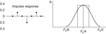
A band-pass filter is derived by multiplying the low-pass coefficients with samples of a sine wave at the center frequency of the band pass. Let’s take our band pass to be centered on the frequency of F^s/4. Samples of a sine wave at this frequency will be at the 0 degree point, the 90 degree point, the 180 degree point, the 270 degree point, and so on. In other words,

0, 1, 0,−1, 0, 1, 0,−1

If we multiply the low-pass coefficients by this sequence we get the following,

0, 0.12, 0,−0.22, 0,+0.12, 0

The impulse response of this circuit is illustrated in Figure F27.5. This looks intuitively right too, because the output can be seen to “ring” at F^s/4, which is what you’d expect from a resonant filter. The derived frequency response is also shown in the diagram.

Figure F27.5. Digital band-pass filter.

Digital frequency domain analysis—the z-transform

The z-transform of a digital signal is identical to the Fourier transform except for a change in the lower summation limit. In fact, you can think of ‘z’ as a frequency variable that can take on real and imaginary (i.e., complex) values. When the z-transform is used to describe a digital signal, or a digital process (like a digital filter), the result is always a rational function of the frequency variable z. That’s to say, the z-transform can always be written in the form:

where the z’s are known as “zeros” and the ‘p’s are known as “poles.”

A very useful representation of the z-transform is obtained by plotting these poles and zeros on an Argand diagram; the resulting two-space representation is termed the “z-plane.” When the poles and zeros are plotted in this way, they give us a very quick way of visualizing the characteristics of a signal or digital signal process.

Problems with digital signal processing

Sampled systems exhibit aliasing effects if frequencies above the Nyquist limit are included within the input signal. This effect is usually no problem because the input signal can be filtered so as to remove any offending frequencies before sampling takes place. However, consider the situation in which a band-limited signal is subjected to a nonlinear process once in the digital domain. This process might be as simple as a “fuzz”-type overload effect, created with a plug-in processor. This entirely digital process generates a new large range of harmonic frequencies (just like its analogue counterpart), as shown in Figure F27.6. The problem arises that many of these new harmonic frequencies are actually above the half-sampling frequency limit and get folded back into the pass-band, creating a rough quality to the sound and a sonic signature quite unlike the analogue “equivalent” (see Figure F27.7). This effect may account for the imperfect quality of many digital “copies” of classic analogue equipment.

Figure F27.6. Generation of harmonics due to nonlinearity

Figure F27.7. Aliasing of harmonic structure in digital, nonlinear processing.

Reference

[1] Brice, R., ‘Audio mixer design’, Electronics and Wireless World, July, 1990.