Chapter | eight
Time Weighting
CHAPTER OUTLINE
The Time Factor in Program Level Meters
Most instruments that display levels create the value displayed through an RMS averaging of the signal over time. In practice, two different methods are used to create the averaged signal, namely linear and exponential averaging. The term time weighting refers to the time window that is used for the creation of the value displayed.
LINEAR AVERAGING
With linear (time) averaging, an average level is created as a simple RMS value of the signal within a given period of time, for example 2 seconds. The weighting for linear averaging is shown in Figure 8.1.
On instruments that are used for acoustic measurements of sound, there is typically an option with a selection of averaging times to choose from: 70 ms, 250 ms and 2 s corresponding to the terms I (impulse, not widely used anymore), F (fast), and S (slow), respectively.

FIGURE 8.1 Principle of linear time weighting: the signal that occurs within the time window is averaged.
For measurements with program level meters for audio recording and transmission, the averaging times used are typically 0.1 ms (fast), 10 ms (standard PPM), 300 ms (VU meter), and 400 ms (LU meter, short term).
EXPONENTIAL AVERAGING
With exponential averaging, the weighting is an exponential function, which, as opposed to linear averaging, does not extend over a fixed period of time. The RMS signal created will thus “remember the past,” but in such a manner that events that lie far away in the past will have a lesser weight than events that have just occurred.
Exponential weighting is shown in Figure 8.2. With exponential averaging, the concept of a time constant is used rather than a time period for averaging. The time constant is a measure of how fast the exponential function “dies” out. Or more precisely, it specifies the time before the exponential function is reduced to 69% of its beginning value.
In connection with the acoustic measurement of sound, there normally is an option to select time constants of 125 ms (fast) and 1 s (slow), as well as an option for impulse weighting.
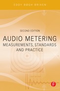
IMPULSE
Impulse weighting differentiates itself from fast and slow weighting by the fact that it contains a peak detector. It is thus the peak value rather than the RMS value that is decisive for the impulse value displayed when the instrument or meter is in I, or impulse, mode. As the name suggests, this form of weighting is intended for the measurement of impulse noise. The time constant is small (35 ms), and a peak detector with an ensuing long time constant (1.5 s) will ensure that impulses will take a long time to “die” out. This form of level display is used, among other things, for the measurement of noise in the external environment, for example when measuring noise from shooting ranges. However, it must be mentioned that the term “I” is gradually finding its way out of the standards. Instead most standards now refer to “peak” measurements, which are displayed with a hold function that leaves the indicator at the max peak detected during the measurement. Depending on national legislation this value is measured using A- or C-frequency weighting.
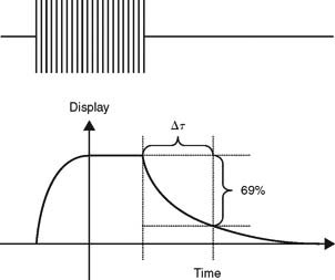
FIGURE 8.2 Principle of exponential averaging.
PEAK
In many countries the measurement of impulse “I” at the workplace has been superseded by the measurement of the peak level. In this case a frequency network (A- or C-weighting) may or may not be used. The peak measurement is supported by a hold function that maintains the highest peak level measured until the next reset.
THE TIME FACTOR IN PROGRAM LEVEL METERS
In program level meters, time weighting and integration time are defined in a slightly different manner as compared to equipment for acoustic measurements.
The integration time is defined in the standards as the time it takes for a signal to reach close to full amplitude. Or, to be more precise, the IEC standard (IEC 60268-10) as an example states that the integration time is the time it takes a 5 kHz sinusoidal burst at reference level to reach a display 2 dB under that reference level. There must be a silent interval between each tone burst large enough that the instrument can settle back to its minimum.

FIGURE 8.3 Leq of a time-varying sound pressure level.
In order to be able to see what the level was when it was there, a fallback time can also be defined. This is the time that elapses from a constant signal being broken until the display reaches a specific lower point on the scale. This can typically be specified in dB/s.
EQUIVALENT LEVEL, Leq
Leq expresses the energy equivalent level. The Leq value is an average value of (on an energy basis) the level over a longer interval of time (minutes to hours). This concept is used in connection with acoustic measurements of sound; however, Leq is also used in connection with electrical measurements for calculation of the loudness of program material. Normally the value is calculated from a frequency-weighted signal, e.g., IEC A (acoustical measurements) or ITU K-weighting (loudness, long term, program material):
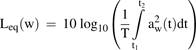
where
w = frequency weighting, e.g., IEC A or ITU k
aw(t) = amplitude of the weighted curve signal
t2– t1 = integration time